Modelling growth of Norway spruce on former agricultural lands in Latvia

(1)

Southern Swedish Forest Research Centre

Modelling growth of Norway spruce on

former agricultural lands in Latvia

Andis Zvirgzdiņš

Master thesis • 30 credits

Euroforester

Master Thesis no. 313 Alnarp, 2019

(2)

(3)

Modelling growth of Norway spruce on former agricultural lands

in Latvia

Andis Zvirgzdiņš

Supervisor: Urban Nilsson, SLU, Southern Swedish Forest Research Centre

Assistant supervisor: Jānis Donis, Latvian State Forest Research Institute “Silava”

Assistant supervisor: Ignacio Barbeito, SLU, Southern Swedish Forest Research Centre

Examiner: Eric Agestam, SLU, Southern Swedish Forest Research Centre

Credits: 30 credits

Level: Advanced level A2E

Course title: Master Thesis in Forest Science

Course code: EX0929

Programme/education: Euroforester Master Program SM001

Course coordinating department: Southern Swedish Forest Research Centre

Place of publication: Alnarp

Year of publication: 2019

Cover picture: Andis Zvirgzdins

Online publication: https://stud.epsilon.slu.se

Keywords: Norway spruce plantations, young stands, height

development, generalized algebraic difference approach, growth simulationsa

Swedish University of Agricultural Sciences Faculty of Forest Sciences

(4)

(5)

3

Abstract

Adequate growth forecasts are essential for forest management planning. In order to make such forecasts, accurate growth models are required. Due to the rapid growth of Norway spruce (L.) Karst. planted on former agricultural lands, existing growth models are unable to predict the development of Norway spruce with sufficient accuracy. Therefore, the aim of this study was to develop new height development and diameter models for Norway spruce up to 15 years of age. Data used in development of the models was obtained from twelve Norway spruce plantations established on fertile agricultural lands located in eastern Latvia. Height development was modelled using dynamic site equations derived using the generalized algebraic difference approach (GADA). In total fifteen different equations were estimated using non-linear least-square regression. Diameter models were developed using multiple linear regression. Subsequently, further development of the stands was simulated using stand-level management simulation tool StandWise of Heureka-DSS.

Of the fifteen tested equations, the best fit and prediction statistics were achieved using Chapman-Richards and Sloboda models. However, the best overall performance was demonstrated by Chapman-Richards model. Diameter was estimating with a linear regression model. Stand level projections showed that MAImax for stands considered in this

study varied between 14.7 – 17.6 m3 ha-1 year-1. According to LEV estimates, optimal rotation age of the stands varied between 41 – 48 years.

With the development of height and diameter growth functions, it is now possible to model development of planted Norway spruce stands from 5 years of age. Furthermore, further development of trees with estimated heights and diameters can be modelled using simulation systems such as Heureka-DSS.

Key words: Norway spruce plantations, young stands, height development, generalized

(6)

4

List of abbreviatons

AAL – Abandoned agricultural land ADA – Algebraic difference approach AIC – Akaike information criterion

CAI – Current annual increment CSB – Central Statistical Bureau DBH – Diameter at breast height DSS – Decision Support System

GADA – Generalized algebraic difference approach LEV – Land expectation value

LLC – Limited Liability Company

LSFRI – Latvian State Forest Research Institute MAI – Mean annual increment

MPE – Mean predicton error NFI – National Forest Inventory NPV – Net present value

PCT – Pre-commercial thinning PE – Prediction error

RMSE – Root mean squared error SD – Standard deviation

(9)

7

1. Introduction

1.1 Norway spruce in Latvia: habitat and distribution

Like in many countries within boreal and boreo-nemoral regions of Europe, Norway spruce (Picea abies (L.) Karst.) is one of the most important tree species in Latvia both for economic and ecological aspects. Cultivation of Norway spruce in Latvia goes back a long way – with the first documented records made in the first forest inventories, conducted in the mid-19th century (Lībiete & Zālītis, 2007). Currently, according to NFI data, Norway spruce is the 3rd most common tree species in Latvian forests, accounting for 18.8 % of the total growing stock (CSB, based on NFI of 2014). Norway spruce is the most productive species in Latvia, with mean annual increment (MAI) of 7.8–8.8 m3_ha-1_year-1_{on average,}

but on very suitable (fertile site conditions), MAI can reach up to 15 m3_ha-1_year-1 _(Bisenieks,

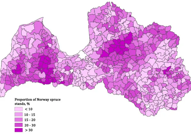
1997; Zviedre, 1999). In terms of distribution of the species, Norway spruce can be found throughout the country (Fig. 1), what can be explained with favourable growth conditions in Latvia (Lībiete & Zālītis, 2007; Zeltiņš, 2017).

Figure 1. Proportion of Norway spruce stands in municipalities of Latvia (Pilvere, 2013).

The distribution of Norway spruce stands in Latvia is not uniform due to differences in suitability of growth conditions as well as due to implementation of management of different goals and intensity. Norway spruce can grow on a variety of site conditions forming both monocultures and mixed stands. In mixed stands it is most commonly found together with Scots pine (Pinus sylvestris), Silver birch (Betula pendula), Downy birch (Betula pubescens) and European aspen (Populus tremula) (Zeltiņš 2017), but it can also be found in mixtures with Grey alder (Alnus incana) and Black alder (Alnus glutinosa), and in rare instances with

(10)

8

Pedunculate oak (Quercus robur) and European ash (Fraxinus excelsior). In a study conducted by Laiviņš (2005), he found that slightly higher proportion of Norway spruce stands in Latvia is observable on highland terrains due to more suitable and nutrient rich soil (clay loam and sandy loam) and more continental climate preferred by this particular species. In addition, Laiviņš (2005) indicated that the most favourable sites for Norway spruce are mesic.

1.2 Growth of Norway spruce

In general terms, Norway spruce is able to grow and show quality performance on a variety of site conditions (Caudullo et al., 2015). In order for the development of Norway spruce to be successful, site conditions must meet the demands of the tree species over the whole rotation period (Rehschuh et al., 2017). In accordance with Bušs (1976; 1981), forest sites on fertile dry mineral soils (Vr – Oxalidosa, Gr - Aegopodiosa), wet mineral soils (Vrs

- Myrtilloso–polytrichosa), drained mineral soils (Ap - Mercurialiosa mel.) and drained peat

soils (Kp - Oxalidosa turf. mel.) are suitable for growing Norway spruce, while Zviedre (1999) indicated that forest sites on dry mineral soils and drained peat soils are the most favourable and productive for Norway spruce, but sites on wet mineral soils and peat soils are less suitable but capable of forming productive stands. In a more recent study by Lībiete & Zālītis (2007), they determined that Norway spruce, as a dominant species, can form stands on fertile forest site types on dry mineral soils and both drained mineral and drained peat soils, what to a large extent confirms the findings of previous studies. The above said coincides with the fact that Norway spruce is capable of being productive on a variety of site conditions. However, in other studies conducted by Zālītis & Lībiete (2003), it was determined that Norway spruce stands growing on wet mineral soils and drained peat soils are less stable and are under bigger risk of breakdown. As a reason for the increased risk of collapsing of the stands is believed to be root rot (Zālītis & Lībiete, 2005).

Norway spruce is considered to be a late successional species (Bušs 1989; Nilsson et

al., 2012; Oberhuber et al., 2015) with slow initial growth. Growth phase of young Norway

spruce stands can be characterized by several stages. According to Lībiete & Zālītis (2007), annual increment of Norway spruce ranges between 10 – 20 cm up until the trees have reached a height of approximately 2 m. Studies carried out in Latvia and abroad have shown that growth in the establishment phase can be affected by a variety of biotic and abiotic factors. Among the most important ones are water and nutrient availability (Zālītis & Lībiete, 2005; Johansson et al., 2011; 2012), climatic factors, soil properties and seedling characteristics (Johansson et al., 2012), browsing, pine weevils and vegetation (Nilsson et

al., 2010).

Following the initial – slow growth phase, a phase of rapid growth ensues in which Norway spruce shows the highest increase in all stand parameters throughout its growth cycle. During this phase volume growth or current annual increment (CAI), on fertile sites, may reach up to 20 m3 ha-1 year-1 (Lībiete & Zālītis, 2007). According to Lībiete (2008), volume growth of Norway spruce is the highest while the mean height of the stand is between 12 – 17 m, often resulting in an accumulation of 200 m3 ha-1 of volume, over the period of 10 years. However, in order to achieve such growth and yield, certain management needs to

(11)

9

be considered. In accordance to Zālītis & Lībiete (2008), intra-specific competition is a decisive factor of the future growth and yield of stands. Therefore, it is recommended to carry out well-timed pre-commercial thinnings. The highest productivity of future crop trees (merchantable timber) can be achieved by reducing the number of trees to 1500 – 2000 trees ha-1 before the mean height of a stand reaches 5 m (Zālītis & Lībiete, 2008). For instance, a young stand which has been thinned (N=1500, H=5.9 m, Age=10), under certain conditions, is capable of producing 18 % or 52 m3 ha-1 more yield than the unthinned stand (N=4000, H=4 m, Age=10) (Zālītis 2006). Furthermore, stands where the mean height has reached or exceeds 10 m, thinning of the smallest trees has no significant effect on the growth of the dominant, future crop trees (Zālītis & Špalte, 2002; Zālītis & Lībiete, 2008). Moreover, beneficial effect of pre-commercial thinning (PCT) on tree growth has been documented in other studies carried out in Latvia as well as in several foreign studies. It has proven to be an important silvicultural treatment for achieving the desirable structure, quality and yield of future stands (Bušs, 1989; Kuliešis & Saladis, 1998; Fahlvik et al., 2005; Weiskittel et al., 2011; Holmstrom et al., 2016).

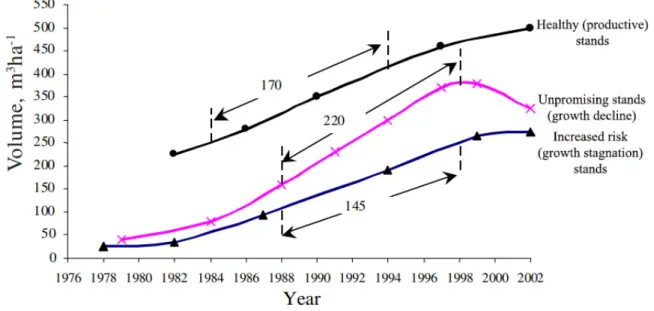
Norway spruce stands in the final stage, what according to Lībiete & Zālītis (2008) occurs at the age of approximately 40 years, may differ partly due to implemented management. On high fertility sites, the total yield at the age of 40 can attain 350 m3 ha-1. In part of the stands, intensive volume growth of around 10 m3 ha-1 continues reaching a yield of up to 500 m3 ha-1 at the end of the rotation (80 years), while in others, significant decline in growth can be observed with CAI being close to zero or even negative and stands on the brink of breakdown (Fig. 2) (Lībiete & Zālītis, 2007; Lībiete, 2008).

Figure 2. Volume growth trends in 30 – 50 year-old Norway spruce stands (Lībiete &

(12)

10

Growth and yield of Norway spruce depends on several site (resource supply) and species (acquisition and resource-use efficiency) related factors. In a study conducted in Latvia, Lībiete & Zālītis (2007) determined that for 30-50 year old Norway spruce stands, largest reciprocal effect or 70 % of the variation of integral growth index i×r (i is annual ring mean width, r is linear correlation coefficient) of Norway spruce could be explained with the ecological requisites of the species, while growth conditions accounted for 30 % (Lībiete & Zālītis, 2007). According to this study, the lowest growth potential of Norway spruce was found for stands growing on drained peat soils, but the highest – for stands growing on drained mineral soils. Decline in production on peat soils could be explained with less suitable soil conditions, i.e. poorer aeration of soil and higher soil humidity in the top layer. In an earlier study by Zālītis (1968), it was determined that on drained peat soil, up to 15 m from the draining-ditch Norway spruce shows the same yield as Scots pine, but beyond, volume growth of Norway was considerably lower than for Scots pine. With that being said, formation of Norway spruce stands on wet mineral soils and drained peat soils is not deemed as imprudent, but species ecological requirements in conjunction with certain management operations should be considered when establishing stands on the respective site conditions.

1.3 Establishment and growth of Norway spruce on AAL

In Latvia, there are more than 300 thousand ha of abandoned agricultural land (AAL), with the highest proportion being in the region of Latgale ~ 27 % (MEPRDRL, 2016). High soil fertility and potentially high production capacity are probably the main reasons for increased interest in growing Norway spruce on AAL. In addition, since 2015 State and EU subsidies are available for establishing forests on former agricultural lands. Furthermore, Norway spruce is one of the most commonly used tree species in plantation establishment, accounting for 35 % or 945 ha planted in 2017 (State Forest Service, 2018).

Norway spruce can grow on a variety of site conditions; however, it best performs on mesic, nutrient-rich soils. Having said that, excessively wet, waterlogged sites as well as nutrient-poor sites should be avoided. Planting Norway spruce on unsuitable sites (parts of the stand) may result in increased mortality of the seedlings, growth stagnation and reduced production, as seen in some of the stands surveyed in this study. According to Daugaviete et

al. (2017), selection of suitable sites may increase the production of Norway spruce

established on plantations by 61 %.

Selecting genetically superior forest reproductive material is of considerable importance in increasing productivity of Norway spruce plantations. In addition, tree selection and genetic modification may increase the resistance of tree species against certain diseases, provided that a sufficient variation of clones is maintained (Daugaviete et al., 2017). The gain in yield using genetically modified material in Latvia is around 10 % (Zeltiņš, 2017). Gain in yield may also depend on site properties and geographical position of the sites. According to Daugaviete et al. (2017), use of genetically improved seedlings may increase the production of Norway spruce established on agricultural lands by 17 %.

Soil scarification is one of the most important silvicultural practices to increase the success of seedling establishment (Johansson et al., 2012). Soil scarification can improve

(13)

11

seedling establishment and survival by: 1) reducing competition from field vegetation; 2) Increasing soil temperature; 3) Decreasing soil density; 4) Increasing soil moisture and mineralization; 5) reducing seedling mortality caused by pine weevil; 6) reducing frost damage (Sundheim Fløistad et al. 2017). In addition, in both Latvian and Swedish studies it has been found that, soil mechanical preparation has a positive effect on the height growth of Norway spruce (Johansson et al. 2012; Lazdiņa, 2018).

Vegetation on the ground cover is a serious competitor for young Norway spruce seedlings. According to Daugaviete et al. (2017), ground vegetation restricting measures are necessary to promote root development and further growth of Norway spruce seedlings. In Latvia, use of herbicides on agricultural lands is permitted, therefore it is highly recommended to eradicate weeds on agricultural lands using herbicides before planting. Researchers from Latvian State Forest Research Institute (LSFRI) have found that 3 years after planting on average, the survival rate of Norway spruce seedlings using herbicides as weed-restricting treatment, is within 99 % (Daugaviete et al., 2017).

After the establishment phase, it does not take long until the intra-specific competition starts between the trees. Competition between trees can be regulated by performing pre-commercial thinnings (PCT’s). As indicated before, well-timed PCT’s are of high importance for the development of future crops trees (merchantable timber). According to Daugaviete et al. (2017), well-timed thinning operations (PCT’s; commercial thinnings) may increase the production of future crop trees by 8 %.

Productivity of Norway spruce plantations can also be increased by fertilization. However, type of fertilizer, quantity of fertiliser used as well as time of application (frequency) has to be considered to achieve best results overall. Fertilization has been found to have a notable effect on growth of Norway spruce on forest sites in Latvia (Jansons et al., 2016; Okmanis et al., 2016). As reported by Daugaviete et al. (2017), the largest height and diameter increment was observed on fertilized Norway spruce sites, compared on unfertilized ones.

1.4 Growth and yield models

Growth of the trees is an immensely complex, biological process in which they extend their successive layers of growth in both height and in diameter over a given time period (Punches, 2004), whereas yield is a measure, which quantifies these layers of growth or final dimensions of trees at the end of a certain period specifying the total volume production. Consequently, growth and yield models are used to describe the complex processes in the forest and predict the future status of the forest at any given time. Both growth and yield are mathematically related – growth is determined by solving a yield equation (if yield is y, growth is the derivative dy/dt), which in many cases allows to transform models from one form to another (Vanclay, 1994).

There are different kind of growth models, differing in the type of data used and the method of construction (Burkhart & Tome, 2012). Commonly, models are divided into two groups: empirical and mechanistic models, but as indicated by Weiskittel et al. (2011), a

(14)

12

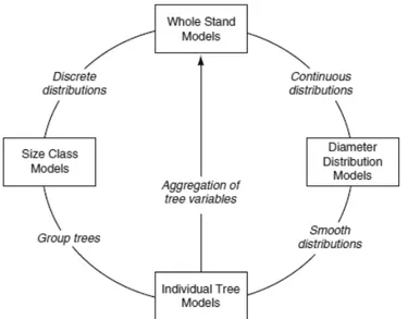
more useful metric of differentiation would be by dividing forest stand models into four categories: 1) statistical, 2) process, 3) hybrid and 4) gap models since all models are on a spectrum of empiricism (Weiskittel et al., 2011). The word empirical refers to a method of obtaining data using observation senses and scientific instruments if necessary. In forestry, this method has been and still is an integral part in construction of growth models as most models are built upon observations collected during surveys or different experiments (Egbäck, 2016). Furthermore, collection and analysis of this type of population (trees in a forest stand) descriptive data allows to estimate statistical variability of certain parameters (Weiskittel et al., 2011). Depending on the level of detail they provide, several modelling approaches can be distinguished. Fundamentally, two types of forest growth models can be recognized: individual-tree and whole-stand (Munro, 1974), but no classification system of modelling approaches can be fully satisfactory as there are various modelling approaches differing in level of resolution or modelling entity. (Burkhart & Tome, 2012). Most common modelling approaches can be regarded in Figure 3.

Figure 3. Classification of the most common modelling approaches and linkages bewteen

them (Burkhart & Tome, 2012).

Whole stand models are some of the oldest and most widely used growth and yield models (Weiskittel et al., 2011). It goes way back, when the first yield tables were developed using data obtained from sample plots located in stands of varying ages representing various site qualities (Burkhart & Tome, 2012). Whole stand models are easy to develop and apply. In addition to that, they are often highly accurate in describing single species, even-aged stands. Whole-stand growth models can be constructed using stand variables such as basal area, site index, stand density index, stand diameter, stand age and number of stems (Sharma, 2013). Notwithstanding, such models have a limited ability to describe complex stand structures (Weiskittel et al., 2011; Qin & Cao, 2006; Garcia 2001), mixed species, and forest silvicultural treatments accurately which can be explained by the applied methods describing such conditions. Accordingly, in many regions of the world, individual tree models, also known as tree-level models have become like the new standard for modelling growth and yield. The reason for this is their flexibility and ability to accurately characterize growth

(15)

13

under a range of stand conditions (Weiskittel et al., 2011). Using tree-level based modelling it is possible to describe different combinations of species mixtures and stand structures, management regimes and regeneration methods (Burkhart & Tome, 2012). In addition, tree-level models are superior to other modelling approaches in characterizing impacts of different damaging agents (Weiskittel et al., 2011). However, tree-level modelling approach requires more detailed data for their development which in most cases makes the data collection procedure more expensive. Furthermore, error compounding is potentially greater for tree-level models (Weiskittel et al. 2011), which can be particularly observed when this detailed information obtained from tree-level models is used in the construction of stand-level models (Cao, 2014). Tree stand-level models can either be distance dependent and distance independent. Distance dependent models require spatial coordinates of all trees, while distance-independent models assume and average spatial pattern of trees (Weiskittel et al. 2011). Most tree-level models are based on radial growth at breast height due to the fact that radial growth is more affected by competition than height growth (Sharma, 2013). As a result, only few individual tree level models have been constructed using height growth as base variable (e.g. Pretzsch et al., 2002; Fahlvik & Nyström, 2006; Nord-Larsen, 2006b; Uzoh and Oliver, 2006; Ritchie and Hamann, 2008; Vaughn et al., 2010).

Irrespective of their level of detail, growth models can also be categorized between deterministic or stochastic. Deterministic growth models, regardless of the number of modelling times, will always return the same output value, provided that the initial values remain unchanged. On the contrary, stochastic models, by incorporating a random element, will return multiple, different predictions in successive runs each with a specific probability of occurrence (Weiskittel et al., 2011; Vanclay, 1994). For instance, contrary to deterministic models, which estimate only one result of the expected growth of a forest stand, stochastic models, by including natural variation characteristic of the environment, estimate several, different growth scenarios. Despite differences between both types of models, they can be used complementarily, providing a more complete understanding of growth processes (Vanclay, 1994).

1.4.1 Height growth modelling

Height is an immensely important tree and site descriptive variable and is often used as input parameter of models or decision support systems (Sharma & Breidenbach, 2015). Various methods and modelling approaches have been used to capture height growth patterns and establish reliable tools, which could be used for forest management planning related decision-making, i.e. scheduling of harvesting operations, planning and evaluation of different silvicultural treatments, etc.

Height growth of co-dominant and dominant trees is the most commonly used indicator of site quality. Dominant height is believed to be independent of stand density and thinning operations, provided it is thinning from below (Skovsgaard & Vanclay, 2008, Burkhart & Tome 2012). In addition, there is strong correlation between height growth and volume production. Therefore, dominant height at a given reference age may be used as a stand productivity descriptive measure (Sharma, 2013). The top height-production relationship is based on Eichhorn’s law or Eichhorn’s hypothesis (Eichhorn, 1904),

(16)

14

indicating that the total production of a fully-stocked stand (net volume production) is a function of its height (Fontes et al., 2003).

Dominant height growth models or site index models can be developed using two modelling approaches: the traditional – base-age specific approach and base age invariant approach. Models based on base-age specific approach are developed using height and a common reference age. Although, base age-specific modelling approach has been widely used for modelling site index, in certain cases, it suffers from inaccurate predictions. Due to the common reference age, in case height is not measured at that specific age, this method requires the use of interpolation or extrapolation to determine height (Sharma, 2013), thus leading to biased prediction results (Weiskittel et al., 2011). As a result, Bailey and Clutter (1974) developed base-age invariant modelling approach – algebraic difference approach (ADA), which allows the use of various types of data for application and parametrization as well as height can be predicted at different ages of the stand (Wieskittel et al., 2011) without significantly affecting the accuracy of predictions. In ADA modelling approach, base equations are described by one site-specific parameter, for which a solution is derived from the base model (Liziniewicz et al., 2016). Models derived from ADA approach may produce curves with a single asymptote, also known as anamorphic curves (Sharma, 2013). Based on the work of Bailey & Clutter (1974), Ciezewksi and Bailey (2000) introduced a generalization of ADA – generalized algebraic difference approach (GADA). It was done by expanding the base model with a purpose to make data and theories of modelled phenomena more inclusive. Compared to ADA, GADA provides more flexible dynamic equations, suitable for a wide range of growth and yield models (Ciezewksi 2002). The GADA method allows derivation of flexible dynamic functions, which are base-age invariant with predicted height equal to site index at base age (Burkhart and Tome 2012). In GADA modelling approach, more than one site-specific parameter can be solved with an equation derived from the base model (Liziniewicz et al., 2016). In case more than one site-specific parameter is solved with an equation, generated models are polymorphic with varying asymptotes (Ciezewski, 2003; Ciezewksi et al., 2007, Liziniewicz et al., 2016). GADA modelling approach has been widely used in the construction of dominant height (site index) growth models for different species and has proven to be reliable (Adame et al., 2006; Martin-Benito et al., 2008; Bravo-Oviedo et al., 2008; Nord-Larsen et al., 2009; Sharma et al., 2011; Perin et al., 2013; Liziniewicz et al., 2016; Feracco Scolforo et al., 2016).

1.4.2 Growth modelling in Latvia

Adequate growth forecasts are essential for forest management planning (Donis, 2016). Although, several studies have been carried out on the growth of Norway spruce in Latvia (Zālītis 1968; Zālītis, 2006; Zālītis & Lībiete, 2007; Zālītis & Lībiete, 2008; Lībiete, 2008), range of models that would accurately describe different growth-related processes is imperfect. Moreover, the changing climate has resulted in new weather patterns (Jansons 2011; 2015, Avotniece et al., 2017) and trees no longer follow the growth patterns they did 20 – 30 years ago, therefore, there is a need to update the existing growth models as well (Donis et al., 2015; Donis & Šņepsts 2015; Donis, 2016).

(17)

15

Probably, the oldest and most widely used tools to predict forest growth are growth and yield tables. In the most commonly used growth and yield tables, forest stand was structured into dominant layer and sub-layer (supressed trees). Dominant layer was described by mean height and diameter, basal area, form factor, number of stems and volume while sub-layer was only explained by volume. Furthermore, these growth and yield tables only described fully stocked even-aged monocultures. Growth and yield tables used in Latvia were obtained by interpolating the growth and yield tables initially constructed by Vargas de Bedemar (1850) for N-W regions of Europe and by Schwappach (1908) for Northern Germany (Skudra, 2005). However, growth and yield tables suffer from a substantial drawback – they are unable to predict the growth of diverse, structurally complex forest stands with sufficient accuracy.

Requirements of modelling dataset (type, quality, size) largely depend on the type of model constructed (Weiskittel et al., 2011). In Latvia, most models are statistical models based on empirical data. Current annual increment (CAI) growth models constructed in Latvia may be based on different data collection methods: permanent plot method, sample tree method, boring (increment core) method and cameralistic method (Donis et al., 2015, Liepa, 2018). Hitherto, growth (CAI) models used in Latvia (Matuzānis 1988, Liepa 1996) have been constructed to a large extent based on increment cores obtained from one-time sample plots visited around 1960’s – 1970’s (Donis 2016). These sample plots were placed in stands varying in age, density and site index (Matuzānis, 1985). According to Donis (2016), these models are unable to accurately predict mortality and thus growth as a whole. Bisenieks (2010) considers that data from periodically re-measured long-term permanent sample plots is sine qua non in the development of reliable growth models. Furthermore, as reported by Donis (2015), National Forest Inventory (NFI), which is a permanent and repeated systematic sample plot inventory, provides most of the variables needed to develop growth models. Consequently, NFI data has been used in the development of several growth models, e.g. Donis et al., (2015) developed CAI and natural mortality models for six different species, including Norway spruce. Equations developed in the study by Donis et

al., 2015 can be used to forecast growth of stand strata, but they are not suitable for predicting

mortality caused by natural disturbances such as forest fires, storms, etc. In the most extensive study so far, Donis (2016; 2017; 2018) worked on the development and improvement of multiple stand level growth models. Based on data obtained from NFI, mean height (Hmean) and dominant height (Hdom) growth models as well as basal area (BA) and

quadratic mean diameter (Dq) growth models were developed for Norway spruce and five

other tree species. Height growth models (Hdom, Hmean) were developed using GADA

modelling approach, as suggested in previous reports (Donis, 2011; 2014; 2015). GADA is a flexible modelling approach, which allows to construct height growth models using only stand height and age, without using information about site index (SI) (Donis, 2018).

In order to be able to accurately describe complex stand structures, species mutual interactions as well as effect of different management regimes of varying intensity, individual-tree models are needed. Based on the knowledge obtained from analysing individual-tree models constructed in Sweden and Finland, Donis (2018) has developed

(18)

16

several individual-tree models for Latvian conditions. For modelling of individual-tree height growth, Donis (2018) provisionally recommends the use of mean height model developed using Hossfled IV equation of GADA.

1.5 Simulations of growth and yield using forest growth simulators

Long-term forest management planning is an immensely complex task (Wikström et., 2011), that requires accurate forecasts of the further development of forest trees and stands. Such forecasts can be obtained by forest growth simulators, which using the underlying models, biometrically and mathematically reproduce the biological growth process (Blatert

et al., 2016). Growth and yield forecasts are usually simulated periodically, i.e. all stand

descriptive variables (height, diameter, basal area, volume growth, etc.) are updated after a certain time period, normally 5 years as minimum. In addition, forest growth simulators provide an opportunity to implement different silvicultural treatments and simulate different management regimes. Ideally, in simulations, it is possible to determine not only future growth and yield, but variety of economic and ecological indicators, necessary in the adoption of decisions related to forest management planning.

1.5.1 The Heureka Forestry Decision Support System (DSS)

Heureka-DSS is an empirically based forest growth simulator, developed and hosted by Swedish University of Agricultural Scieneces (Wikström et al., 2011; Subramanian, 2016). Heureka-DSS encompasses many of the empirical growth models developed in Sweden (Fahlvik et al., 2014; Egbäck, 2016). The system consists of three main applications: • Heureka StandWise – a stand-level management simulation and visualization tool,

which allows to simulate development of one stand at a time. Stand development is simulated periodically, with minimum time step of five years. During the simulation process, different silvicultural treatments can be specified, period by period. • Heureka PlanWise – a forest-level (landscape-level) analysis and planning tool,

that provides an opportunity to simulate development of several stands at a time with a minimum time span of five years. In addition to the possibility to analyze different management scenarios, this application has a built-in optimization tool. • Heureka RegWise – a regional-level (national-level) planning tool for long-term

analysis of large geographical areas. RegWise long-term forecasts are mainly based on national forest inventory (NFI) data, but also digital maps and data obtained from remote sensing are used. Regwise allows to forecast future status and production of different ecosystem services of large scale forest areas, depending on the chosen forest management approach (SLU, 2016; Subramanian, 2016).

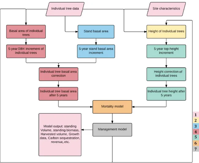
All three of the applications listed above use the same set of sub-models (Fig. 4) for predicting site and stand data (e.g. site index, tree age), growth and mortality (Fahlvik et al., 2014). More in-depth description of the underlying sub-models of Heureka-DSS can be found in the studies of Fahlvik et al. (2014) and Subramanian (2016).

(19)

17

Figure 4. Schematic diagram of Heureka-DSS and its underlying models. Different colours in the scheme represent different components (sub-models) of Heureka simulation system. They are as follows: input-output module (1), estimation of individual tree heights at the start of the simulation (2), stand basal area increment function (3), five-year DBH increment functions for individual trees (4), height increment function for individual trees (5), mortality model (6) and management model (7) as adopted from Subramanian (2016).

Simulation results of the analyzed stands or forest areas are given in the form of tables, maps and graphs. Different forest stand descriptive variables, such as Stand age (years), Dgv

(cm), Hgv (m), Volume (m3ha-1), Net Revenue (SEK/ha-1), can be selected by the user, as

well as graphs and maps can be created or modified at its own discretion. Furthermore, different silvicultural treatments can be implemented or management scenarios generated using built-in control categories of Heureka-DSS.

1.6 Aims of the thesis

The main objective of this study was to study growth of Norway spruce planted on former agricultural lands and develop diameter and height development models describing growth from five to fifteen years of age. Subsequently, with the set of models developed to estimate height and diameter of trees at the age of fifteen years, analyse further stand development using stand growth simulator.

(20)

18 The main aims were:

1. Construct a model for height development of Norway spruce from five to fifteen years of age.

2. Develop a model, which would accurately estimate DBH of Norway spruce at the age of 15 years.

3. Evaluate stand growth and determine the optimal rotation age of stands considered in this study.

1.6.1 Schematic diagram of thesis structure

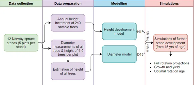
The process of developing this master’s project, including all tasks, is depicted schematically in Figure 5. The work consists of 4 main stages: the first two stages are Data

collection and Data preparation, where data is being prepared and arranged for the

construction of the models. The last two: Modelling and Simulations are stages where the tree main tasks of this study are fulfilled.

(21)

19

2. Materials and methods

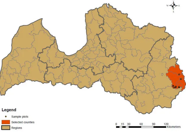
2.1 Study area

The study was carried out in the eastern part of Latvia – Latgale – a region located at the frontier of Belarus and Russia. In total, 12 Norway spruce stands were selected within the latitude of 56°12' and 56°35' and longitude of 27°44' and 27°58', located in the 3 easternmost counties of Latvia – Ludza, Cibla and Zilupe (Fig. 6).Typically for the continental climate, the climate in this part of the country is more diverse than it is in the rest of the country, i.e. summers are hotter, winters are more severe and the temperature changes more drastically throughout the year with an average annual temperature being approximately + 5.2 °C. (National encyclopedia, 2019). Mean annual precipitation for the area selected for this study (Fig 6., highlighted in red) is between 600 – 650 mm year-1_{, which}

is slightly lower than the mean annual precipitation in the whole country. The area is located relatively high, 160 m a.s.l., while most of the country’s territory (73,5 %), is below 120 m a.s.l. According to genetic soil classification of Latvia, soil in this highland is mainly podzolic (sod-podzolic, sod-podzolic gley soil, eroded podzolic soil) with sandy loam and loam as predominant constituent of soil parent rock.

Fig. 6. Geographical location of the study area.

2.2 Selection of the stands and site description

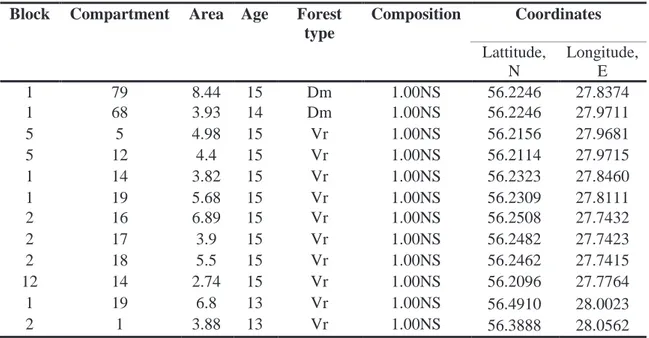
All twelve stands were selected within the area managed by Skogssällskapet Latvia, LLC (Table 1). Several criteria such as age, species composition, forest type was considered when selecting stands. Only pure Norway spruce stands were considered, which in this

(22)

20

research were defined as stands where an admixture of other tree species was below 15 % of number of trees. Further on, stands were selected by soil type. In this study, we focused on stands growing only on dry mineral soils, which according to Latvia’s forest typology developed under guidance of Bušs in 1976 (Liepa et al. 2014) could be classified as – Dm (Hylocomiosa) and Vr (Oxalidosa), the two most common forest types found in Latvia. In Latvia these forest types are often dominated by Norway spruce either in monocultures or in mixtures with other species. Hylocomiosa forest types most often are found on sandy loam, sandy soils but Oxalidosa on clay loam or clay soils. Forests on wet or drained soils were not considered in this research, because the data was not large enough to include soil moisture class in the models. Because many stands were established on former agricultural lands in the early 2000s, the age of the stands varied from thirteen to fifteen years. All of the stands were established by planting (2500 seedlings per ha) and most of the stands have undergone a thorough commercial thinning, but some had only been partially pre-commercially thinned.

Table 1. Selected Norway spruce stands

Note: Vr – Forest type Oxalidosa, Dm – Forest type Hylocomiosa; 1.00NS – 100% Norway spruce; Age was

specified at the time of measurements (2018).

2.3 Data collection

Five sample plots with a radius of 5.64 m (100 m2_{) were placed in every stand. The}

location of the sample plots was generated using geospatial processing tool ArcMap. After placing a buffer zone of ten m from the edge of the stands, sample plots were placed with a quadratic spacing of thirty m. In the sample plots, all trees above two cm in DBH were cross-calipered and depending on the diameter distribution and species present in the plot, height was measured for four to nine trees using a Haglöf Vertex IV hypsometer. Thereafter, two dominant and two co-dominant trees were chosen and cut with a chainsaw. These trees were delimbed, leaving around 5 - 10 cm long twigs so that it was possible to determine positions of the whorls. Following delimbing, annual height growth was measured for every sample tree by attaching a measuring tape to the top of the tree and registering length at every whorl down to the root collar. But in order to determine height increment for every year, height of

Block Compartment Area Age Forest

type Composition Coordinates Lattitude, N Longitude, E 1 79 8.44 15 Dm 1.00NS 56.2246 27.8374 1 68 3.93 14 Dm 1.00NS 56.2246 27.9711 5 5 4.98 15 Vr 1.00NS 56.2156 27.9681 5 12 4.4 15 Vr 1.00NS 56.2114 27.9715 1 14 3.82 15 Vr 1.00NS 56.2323 27.8460 1 19 5.68 15 Vr 1.00NS 56.2309 27.8111 2 16 6.89 15 Vr 1.00NS 56.2508 27.7432 2 17 3.9 15 Vr 1.00NS 56.2482 27.7423 2 18 5.5 15 Vr 1.00NS 56.2462 27.7415 12 14 2.74 15 Vr 1.00NS 56.2096 27.7764 1 19 6.8 13 Vr 1.00NS 56.4910 28.0023 2 1 3.88 13 Vr 1.00NS 56.3888 28.0562

(23)

21

each whorl was calculated going backwards (starting from root collar). Age was recorded by counting tree annual rings on the stump.

2.4. Estimation of height of all calipered trees

Due to the difficult and time-consuming procedure of measuring individual tree height, in stands considered in this study, height was recorded for 4 – 9 trees per plot. However, for starting values in Heureka simulations and for calculation of variable Hsum of diamter model,

it was necessary to determine height of all the trees present in the sample plots. In order to determine height of all trees present in the sample plots, DBH–height relationship was estimated for each sample plot of each stand using height curve for Norway spruce developed by Näslund (1936).

𝐻𝐻 =_{(𝑎𝑎 + 𝑏𝑏 ∗ 𝐷𝐷)}𝐷𝐷3 ₃+ 1.3, (1) where H is height of the tree (m), D is diameter at breast height (cm) and a and b are coefficients of the model. Data from trees with both height and diameter measurements was used for constructing the models. With newly obtained equations height was estimated for all the trees, which had their diameter measured.

2.5 Models

Two different type of models were developed in this study, describing development of planted Norway spruce on former agricultural lands. Height development models were constructed from five to fifteen years of age using height increment data of 240 sample trees. Diameter models weere developed to estimate DBH at the age of fifteen years using measured diameters and tree heights calculated with the DBH–height function.

2.5.1 Height development model

Based on scientific knowledge in the field of research topic and previous studies (Cieszewski et al., 2007; Liziniewicz et al., 2016; Bravo-Oviedo et al., 2008; Scolforo et al., 2016; Martin-Benito et al., 2008; Sharma et al., 2011) in which this method has been used and proven to be capable of achieving good results, the generalized algebraic difference approach (GADA) was used in this study. GADA models used in this study are either based on base equations of fractional form (Hossfeld, King-Prodan and Strand) or exponential form (Chapman-Richards, Korf and Sloboda). In total, fifteen different equations, adopted from Sharma et al. 2011 and Liziniewicz et al. 2016, were tested in this study (Table 2). Amongst fifteen tested equations, five of them were GADA formulations of Chapman-Richards growth equation (equations (F01 – F05)), seven of them (equations (F06 – F12)) were derived from three different base equations of Hossfeld, including F06, developed by Elfving and Kiviste (1997). Of the remaining five equations, two of them were GADA formulations of Korf (F13 – F14) and the last three (equations (F15 – F17)) were GADA formulations of King-Prodan, Sloboda and Strand base equations respectively. The equations presented in this study can be defined by their parameters of the base model form (a1, a2,..., an and H, S,

(24)

22 T ab le 2. B as e m o d el s an d g en er al iz ed al g eb rai c d if fer en ce m o d el s ( G A D A ) u sed i n t h is s tu d y B as e m o d el f o rm S ite -s p eci fi c p ar am et er s S o lu tio n f o r th eo re tic al v ar ia b le X G ADA m o d el f o r m us ed i n es ti m a ti o n o f t h e p a ra m et ers C h ap m an -R ich ar d s: 𝐻𝐻 = 𝑎𝑎1 (1 − 𝑒𝑒( − 𝑎𝑎2 𝑇𝑇) ) 𝑎𝑎3 𝑎𝑎1 = X 𝑋𝑋0 = 𝐻𝐻0 (1 − exp (− 𝑏𝑏2 𝑇𝑇0 )) 𝑏𝑏3 𝑯𝑯 = � 𝟏𝟏 − 𝐞𝐞𝐞𝐞𝐞𝐞 (− 𝒃𝒃𝟐𝟐 𝑻𝑻) 𝟏𝟏 − 𝐞𝐞𝐞𝐞𝐞𝐞 (− 𝒃𝒃𝟐𝟐 𝑻𝑻𝟎𝟎 )� 𝒃𝒃𝟑𝟑 (F 01) 𝑎𝑎2 = X 𝑋𝑋0 = − ln (1 − (𝐻𝐻0 /𝑏𝑏1 ) 1/ 𝑏𝑏3 ) 𝑇𝑇0 𝑯𝑯 = 𝒃𝒃𝟏𝟏 �𝟏𝟏 − �𝟏𝟏 − � 𝑯𝑯𝟎𝟎 � 𝒃𝒃𝟏𝟏 𝟏𝟏/ 𝒃𝒃𝟑𝟑 � 𝑻𝑻/ 𝑻𝑻𝟎𝟎 � 𝒃𝒃𝟑𝟑 (F 02) 𝑎𝑎3 = X 𝑋𝑋0 = − ln (𝐻𝐻0 /𝑏𝑏1 ) ln (1 − exp (− 𝑏𝑏2 𝑇𝑇0 )) 𝑯𝑯 = 𝒃𝒃𝟏𝟏 � 𝑯𝑯𝟎𝟎 � 𝒃𝒃𝟏𝟏 (𝐥𝐥𝐥𝐥 (𝟏𝟏 − 𝐞𝐞𝐞𝐞𝐞𝐞 (− 𝒃𝒃𝟐𝟐 𝑻𝑻) )) (𝐥𝐥𝐥𝐥 (𝟏𝟏 − 𝐞𝐞𝐞𝐞𝐞𝐞 (− 𝒃𝒃𝟐𝟐 𝑻𝑻𝟎𝟎 )) ) (F 03) 𝑎𝑎1 = exp (𝑋𝑋 ) 𝑎𝑎3 = 𝑏𝑏2 + 𝑏𝑏3 𝑋𝑋 𝑋𝑋0 = 1 �𝛹𝛹 2 + �𝛹𝛹 2 − 4𝑏𝑏3 𝛷𝛷 � w h er e 𝛹𝛹 = ln 𝐻𝐻0 − 𝑏𝑏2 𝛷𝛷 and 𝛷𝛷 = ln (1 − exp (− 𝑏𝑏1 𝑡𝑡0 )) 𝑯𝑯 = 𝑯𝑯𝟎𝟎 � 𝟏𝟏 − 𝒆𝒆𝒆𝒆 𝒆𝒆( − 𝒃𝒃𝟏𝟏 𝑻𝑻) 𝟏𝟏 − 𝒆𝒆𝒆𝒆 𝒆𝒆( − 𝒃𝒃𝟏𝟏 𝑻𝑻𝟎𝟎 )� (𝒃𝒃𝟐𝟐 + 𝒃𝒃𝟑𝟑 /𝑿𝑿𝟎𝟎 ) (F 04) H o ssf el d b as ed m ode l o f E lf vi ng a nd K ivi st e ( 199 7) 𝐻𝐻 = 𝑎𝑎1 1 + 𝑎𝑎2 𝑇𝑇 − 𝑎𝑎 3 S ol ve d w it h a n a ss um pt ion t ha t 𝑎𝑎2 = 𝑎𝑎3 /𝑆𝑆 𝑯𝑯 = 𝑯𝑯𝟎𝟎 + 𝒅𝒅 + 𝒓𝒓 𝟐𝟐 + (𝟒𝟒 𝒃𝒃𝟑𝟑 /𝑻𝑻 𝒃𝒃𝟐𝟐)/ (𝑯𝑯𝟎𝟎 − 𝒅𝒅 + 𝒓𝒓) , w h ere 𝒅𝒅 = 𝒃𝒃𝟏𝟏 𝒃𝒃 𝟐𝟐_𝑨𝑨𝒔𝒔𝒔𝒔 an d 𝒓𝒓 = �(𝑯𝑯 𝟎𝟎 − 𝒅𝒅) 𝟐𝟐 + 𝟒𝟒𝒃𝒃𝟑𝟑 𝑯𝑯𝟎𝟎 𝑻𝑻𝟎𝟎 − 𝒃𝒃𝟐𝟐 (F0 5 )

(25)

23 T a b le 2 . (c ont inue d) B as e m o d el f o rm S ite -s p eci fi c p ar am et er s S o lu tio n f o r th eo re tic al v ar ia b le X G ADA m o d el f o r m us ed i n p a ra me te r e sti ma ti o n H os sf el d: 𝐻𝐻 = 𝑎𝑎1 1 + 𝑎𝑎2 𝑇𝑇 − 𝑎𝑎 3 𝑎𝑎1 = 𝑏𝑏1 + 𝑋𝑋 𝑎𝑎3 = 𝑏𝑏2 /𝑋𝑋 𝑋𝑋0 = 1 �𝛹𝛹 2 + �𝛹𝛹 2+ 4𝑏𝑏2 𝐻𝐻0 𝑇𝑇0 − 𝑏𝑏3� , w h er e 𝛹𝛹 = 𝐻𝐻0 − 𝑏𝑏1 𝑯𝑯 = 𝒃𝒃𝟏𝟏 + 𝑿𝑿𝟎𝟎 𝟏𝟏 + 𝒃𝒃𝟐𝟐 /𝑿𝑿𝟎𝟎 𝑻𝑻 − 𝒃𝒃𝟑𝟑 (F0 6 ) 𝑎𝑎1 = 𝑏𝑏1 + 𝑋𝑋 𝑎𝑎3 = 𝑏𝑏2 𝑋𝑋 𝑋𝑋0 = 𝐻𝐻0 − 𝑏𝑏1 1 − 𝑏𝑏2 𝐻𝐻0 𝑇𝑇0 − 𝑏𝑏3 𝑯𝑯 = 𝒃𝒃𝟏𝟏 + 𝑿𝑿𝟎𝟎 𝟏𝟏 + 𝒃𝒃𝟐𝟐 𝑿𝑿𝟎𝟎 𝑻𝑻 − 𝒃𝒃𝟑𝟑 (F0 7 ) 𝑎𝑎2 = X 𝑋𝑋0 = 𝑇𝑇0 𝑏𝑏3 � 𝑏𝑏1 − 𝐻𝐻0 1� 𝑯𝑯 = 𝒃𝒃𝟏𝟏 �𝟏𝟏 − �𝟏𝟏 − 𝒃𝒃𝟏𝟏 �� 𝑯𝑯𝟎𝟎 𝑻𝑻𝟎𝟎 � 𝑻𝑻 𝒃𝒃𝟑𝟑 � (F0 8 ) H os sf el d: 𝐻𝐻 = 𝑇𝑇 2 𝑎𝑎1 + 𝑎𝑎2 𝑇𝑇 + 𝑎𝑎3 𝑇𝑇 2 𝑎𝑎2 = 𝑋𝑋 𝑎𝑎3 = 𝑏𝑏1 + 𝑏𝑏2 𝑋𝑋 𝑋𝑋0 = 𝑇𝑇0 2 (1 − 𝑏𝑏1 𝐻𝐻0 )− 𝑏𝑏1 𝐻𝐻0 𝐻𝐻0 𝑇𝑇0 (1 + 𝑏𝑏2 𝑇𝑇0 ) 𝑯𝑯 = 𝑻𝑻 𝟐𝟐 𝒃𝒃𝟏𝟏 (𝟏𝟏+ 𝑻𝑻 𝟐𝟐)+ 𝑿𝑿𝟎𝟎 𝑻𝑻( 𝟏𝟏 + 𝒃𝒃𝟐𝟐 𝑻𝑻) (F0 9 ) M ons er ud ( 1984) d er ive d b y C ie sz ew ski ( 2001) : 𝐻𝐻 = 𝑎𝑎1 𝑆𝑆 𝑎𝑎2 1 + exp (𝑎𝑎3 − 𝑎𝑎4 log 𝑇𝑇 − 𝑎𝑎5 log (𝑆𝑆 ) 𝑆𝑆𝑆𝑆 𝑙𝑙𝑢𝑢 𝑡𝑡𝑢𝑢 𝑆𝑆𝑢𝑢 𝑓𝑓 𝑆𝑆𝑓𝑓 𝑆𝑆 𝑎𝑎 𝑋𝑋0 = (𝑌𝑌0 − 𝑏𝑏1 )+ �(𝑌𝑌 0 − 𝑏𝑏1 ) 2 + 2𝑏𝑏2 𝐻𝐻0 𝑇𝑇 0 − 𝑏𝑏3 𝑯𝑯 = 𝑻𝑻 𝒃𝒃𝟑𝟑(𝑻𝑻 𝟎𝟎 𝒃𝒃𝟑𝟑 𝑿𝑿 𝟎𝟎 + 𝒃𝒃𝟐𝟐 ) 𝑻𝑻 𝟎𝟎 𝒃𝒃𝟑𝟑 (𝑻𝑻 𝒃𝒃𝟑𝟑𝑿𝑿 𝟎𝟎 + 𝒃𝒃𝟐𝟐 ) (F1 0 ) K o rf: 𝐻𝐻 = 𝑎𝑎1 exp (− 𝑎𝑎2 𝑇𝑇 − 𝑎𝑎3 ) 𝑎𝑎1 = exp (𝑋𝑋 ) 𝑎𝑎2 = (𝑏𝑏1 + 𝑏𝑏2 ) 𝑋𝑋 𝑋𝑋0 = 1 𝑇𝑇 2 0 − 𝑏𝑏3 �𝛹𝛹 + �4𝑏𝑏 2 𝑇𝑇0 𝑏𝑏3 + (− 𝛹𝛹 ) 2 � , w h er e 𝛹𝛹 = 𝑏𝑏1 + 𝑇𝑇0 𝑏𝑏3 ln (𝐻𝐻0 ) 𝑯𝑯 = 𝐞𝐞𝐞𝐞 𝐞𝐞( 𝑿𝑿𝟎𝟎 )𝐞𝐞𝐞𝐞𝐞𝐞 �− � 𝒃𝒃𝟏𝟏 + 𝒃𝒃𝟐𝟐 𝑿𝑿𝟎𝟎 �𝑻𝑻 − 𝒃𝒃𝟑𝟑� (F1 1 )

(26)

24 T a b le 2 . ( cont inue d ) B as e m o d el fo rm S ite -s p eci fi c p ar am et er s S o lu tio n f o r th eo re tic al v ar ia b le X G ADA m o d el f o r m us ed i n p a ra me te r e sti ma ti o n 𝑎𝑎2 = 𝑋𝑋 𝑋𝑋0 = − 𝑙𝑙𝑢𝑢 � 𝐻𝐻0 �𝑇𝑇 𝑏𝑏1 0 𝑏𝑏3 𝑯𝑯 = 𝒃𝒃𝟏𝟏 𝐞𝐞𝐞𝐞𝐞𝐞 �𝐥𝐥𝐥𝐥 � 𝑯𝑯𝟎𝟎 �� 𝒃𝒃𝟏𝟏 𝑻𝑻𝟎𝟎 � 𝑻𝑻 𝒃𝒃𝟑𝟑 � (F1 2 ) Ki ng -P rod an: 𝐻𝐻 = 𝑇𝑇 𝑎𝑎 1 𝑎𝑎2 + 𝑎𝑎3 𝑇𝑇 𝑎𝑎 1 𝑎𝑎2 = 𝑏𝑏2 + 𝑏𝑏3 𝑋𝑋 𝑎𝑎3 = 𝑋𝑋 𝑋𝑋0 = 𝑇𝑇0 𝑏𝑏1 /𝐻𝐻 0 − 𝑏𝑏2 𝑏𝑏3 + 𝑇𝑇 0 𝑏𝑏1 𝑯𝑯 = 𝑻𝑻 𝒃𝒃𝟏𝟏 𝒃𝒃𝟐𝟐 + 𝒃𝒃𝟑𝟑 𝑿𝑿𝟎𝟎 + 𝑿𝑿𝟎𝟎 𝑻𝑻 𝒃𝒃𝟏𝟏 (F1 3 ) S loboda : 𝐻𝐻 = 𝑎𝑎1 exp �− 𝑎𝑎2 exp � 𝑎𝑎3 (𝑎𝑎4 − 1) (𝑎𝑎4 − 1) �� 𝑎𝑎2 = 𝑋𝑋 𝑋𝑋0 = − ln (𝐻𝐻0 /𝑏𝑏1 ) exp � 𝑏𝑏2 (𝑏𝑏3 − 1) 𝑇𝑇 0 (𝑏𝑏3 − 1) � 𝑯𝑯 = 𝒃𝒃𝟏𝟏 � 𝑯𝑯𝟎𝟎 � 𝒃𝒃𝟏𝟏 𝐞𝐞𝐞𝐞𝐞𝐞 � 𝒃𝒃𝟐𝟐 (𝒃𝒃𝟑𝟑 − 𝟏𝟏) 𝑻𝑻 (𝒃𝒃𝟑𝟑− 𝟏𝟏) − 𝒃𝒃𝟐𝟐 (𝒃𝒃𝟑𝟑 − 𝟏𝟏) 𝑻𝑻𝟎𝟎 (𝒃𝒃𝟑𝟑− 𝟏𝟏) � (F1 4 ) S tr an d: 𝐻𝐻 = � 𝑇𝑇 𝑎𝑎1 + 𝑎𝑎2 𝑇𝑇� 𝑎𝑎3 𝑎𝑎1 = 𝑋𝑋 𝑎𝑎2 = 𝑏𝑏1 + 𝑏𝑏2 𝑋𝑋 𝑋𝑋0 = 𝑇𝑇0 �𝐻𝐻 0 − 1 𝑏𝑏3− 𝑏𝑏1 � 1 + 𝑏𝑏2 𝑇𝑇0 𝑯𝑯 = � 𝑻𝑻 𝑿𝑿𝟎𝟎 + 𝑻𝑻( 𝒃𝒃𝟏𝟏 + 𝒃𝒃𝟐𝟐 𝑿𝑿𝟎𝟎 )� 𝒃𝒃𝟑𝟑 (F1 5 ) N o te : H, S ( fi x ed -b ase -ag e S I) , T a nd a1 , a 2 , . .., a n a re p ar am et er s i n b as e m o d el s; b1 , b 2 , ..., bn ar e p ar am et er s i n G A D A m o d el s; H 0 an d H ar e h ei g h ts ( in m ) at ag e T 0 a nd T (i n y ear s) , r es p ect iv el y ; X 0 i s th e so lu tio n o f X f o r i n itia l h eig h t an d a g e.

(27)

25

In the general implicit form H = f (T, T0, H0, b1, b2,…bn), which is the same for all GADA

equations, H0 is an observed height at the observed age T0, while H is a predicted height at

index age T. H is a local parameter, which is estimated using GADA dynamic equations (Liziniewicz et al. 2016). All parameters and equations used to estimate them are presented in Table 2. Base models, from which the relevant dynamic site equations are derived, are represented in the first column. Dynamic site equations, presented in column 4, are the equations used in the construction of height development models and estimation of their parameters. In case, dynamic site equation consist of theoretical variable X, dynamic equation must be supplemented by the solution of it (column 3).

2.5.2 Diameter model

A function for estimating diameter at the age of 15 years was developed using multiple linear regression analysis. Linear model was applied on the following function:

𝑙𝑙𝑢𝑢 𝑑𝑑 = 𝑓𝑓�ℎ, 𝑙𝑙𝑢𝑢ℎ, 𝐻𝐻𝑔𝑔𝑔𝑔, 𝑙𝑙𝑢𝑢𝐻𝐻𝑔𝑔𝑔𝑔, 𝐻𝐻𝑠𝑠𝑠𝑠𝑠𝑠�, (2)

where lnd is a natural logarithm of diameter in cm, h is height, lnh is natural logarithm of height in m, Hgv is basal area weighted mean height, lnHgv is natural logarithm of Hgv, Hsum is sum of

heights of trees larger than the subject tree. Values of h an lnh describe each tree individually, while 𝐻𝐻_{𝑔𝑔𝑔𝑔}, 𝑙𝑙𝑢𝑢𝐻𝐻_{𝑔𝑔𝑔𝑔,} 𝐻𝐻_{𝑠𝑠𝑠𝑠𝑠𝑠} are estimated on a plot level. Basal area weighted mean height (Lorey’s mean height) is introduced because it is more stable compared to the arithmetic mean height and it allows the larger trees to contribute more to the mean. Whereas, 𝐻𝐻_{𝑠𝑠𝑠𝑠𝑠𝑠} is a distance-independent competition index, which describes the intensity of competition between a subject tree and the neighbouring competitors within a plot. 𝐻𝐻𝐻𝐻𝑢𝑢𝐻𝐻_𝑖𝑖 is calculated in the following way:

𝐻𝐻𝐻𝐻𝑢𝑢𝐻𝐻𝑖𝑖 = � ℎ𝑗𝑗, (3)

when ℎ_𝑗𝑗 > ℎ_𝑖𝑖, where ℎ_𝑖𝑖 is the height of the subject tree and ℎ_𝑗𝑗 is height of the neighbouring competitor

2.6 Parameter estimation and other computations

Parameter values for all GADA models or equations were estimated with non-linear least-square regression using R functions nlrob of package ‘robustbase’, nlsLM of package ‘minpack.lm’ and nls function which is a built-in function in R. In order to achieve a better fit, some of the models were tested with two non-linear fitting functions. All the parameters, both site-specific and global, were estimated simultaneously. Diameter model was estimated using linear regression model lm. Other computations, such as evaluation of the models, as well as visual display of the results was performed using R (version 3.5.1).

2.7 Model evaluation

The models developed in this study were evaluated using prediction statistics, graphs of residuals and prediction errors. Height prediction errors were determined by comparing the actual height measurements with the values estimated by models using measured data: models were used to estimate height (H) for every tree at the age of 10 and at the age of 15, if such

(28)

26

records existed. As input data, starting height (H0) of the respective trees at different index ages

was used, e.g. for estimation of height (H) for a tree at the age of 15, starting height (H0) at

different ages (T0 = 5,6,7,8,9,10,11,12,13,14) was used. Statistical accuracy of the models was

evaluated by residual analysis using mean prediction error (MPE), standard deviation (SD) and root mean square error (RMSE). In addition, relative quality of the models was determined by Akaike information criterion (AIC) using the built-in AIC function in R.

2.8 Simulations of the further development of the stands

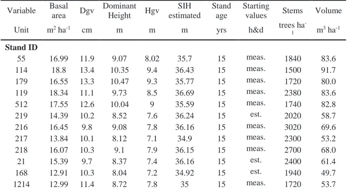
In order to be able to use stand-level management simulator - StandWise and its underlying models for forecasting further development of the stands in Latvian conditions, different variables describing site conditions, such as altitude, latitude, soil moisture, soil texture, vegetation type, had to be specified by approximation based on the location of the study sites. Subsequently, data consisting of tree heights, diameters and site descriptive values were imported into StandWise. Since most of the stands had already reached the age of 15 years, models developed in this study were only used to estimate height and diameter of stands 21, 219 and 168, which were 13, 13 and 14 years old respectively at the time of measurements. With the given starting values, current growth and yield of the stands was estimated at the age of 15 years.

Table 3. Stand data (Forest data)

Variable Basal area Dgv Dominant Height Hgv SIH estimated Stand age Starting

values Stems Volume

Unit m2_ha-1 _cm _m _m _m _yrs _h&d trees ha

-1 m 3_ha-1 Stand ID 55 16.99 11.9 9.07 8.02 35.7 15 meas. 1840 83.6 114 18.8 13.4 10.35 9.4 36.43 15 meas. 1500 91.7 179 16.55 13.3 10.47 9.3 35.77 15 meas. 1720 80.0 119 18.34 11.1 9.73 8.5 36.69 15 meas. 2380 83.6 512 17.55 12.6 10.04 9 35.59 15 meas. 1740 82.8 219 14.39 10.2 8.52 7.6 36.24 15 est. 2020 58.7 216 16.45 9.8 9.08 7.8 36.16 15 meas. 3020 69.6 217 13.84 10.1 8.12 7.1 34.9 15 meas. 2300 53.2 218 16.07 10.3 9.1 7.9 36.15 15 meas. 2700 68.0 21 15.39 9.7 8.37 7.4 36.16 15 est. 2400 61.4 168 12.91 10.3 8.04 7.2 34.92 15 est. 1940 49.7 1214 12.99 11.4 8.72 7.8 35 15 meas. 1720 53.7

Note: Data in this table is based on fully stocked sample plots; Starting values: meas. is measured and est. is

estimated; SIH (H100) - calculated based on site factors for Norway spruce (Hägglund and Lundmark 1977)

Subsequently, the course of growth of each stand was simulated by applying a standard management regime: 2 – 3 thinnings from below (relative diameter ratio – 0.9) with an intensity of 30 – 35 %. Simulation results were estimated and demonstrated for every 5 year period in the form of a new status for the stand, timber production and economy, represented with previosly selected stand variables. Financial value of the stands was displayed by Total Cost

(29)

27

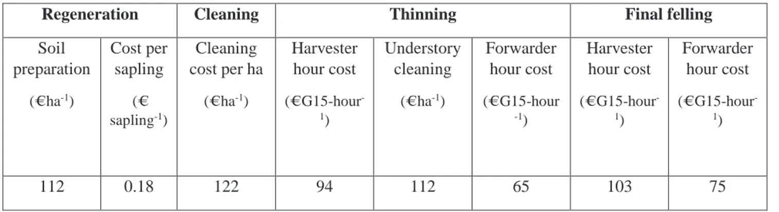
and Net Revenue. In order to make the results more admissible, default timber price list was replaced by a timber pricelist based on situation currently existing in Latvian roundwood market (Table 4). In addition, bucking specifics, i.e. minimum and maximum length and diameter of sawlogs and pulpwood were adjusted based on the provided pricelist (Table 4). The Costs of different management operations such as regeneration, cleaning, thinning largely coincided with the costs in Latvia (Table 5). More specific indicators such as technological parameters (machine related) were assumed to be similar in Sweden and Latvia, therefore they were not modified.

Table 4. StoraEnso timber pricelist for Norway spruce in Latvia, 2019 (€ m-3₎

Table 5. List of adjusted costs used in the simulations (€)

Regeneration Cleaning Thinning Final felling

Soil preparation (€ ha-1₎ Cost per sapling (€ sapling-1₎ Cleaning cost per ha (€ ha-1₎ Harvester hour cost (€ G15-hour -1₎ Understory cleaning (€ ha-1₎ Forwarder hour cost (€ G15-hour -1₎ Harvester hour cost (€ G15-hour -1₎ Forwarder hour cost (€ G15-hour -1₎ 112 0.18 122 94 112 65 103 75

Note: Cost table obtained from CSB of Latvia

Length (m) Diam. (cm) 3.6 3.9 4.2 4.5 4.8 5.1 5.4 5.7 6.0 Roundwood 9 –11.9 53 53 53 53 53 50 50 50 50 12 – 13.9 58 58 58 58 58 55 55 55 55 14 – 17.9 69 69 69 69 69 69 69 69 69 18 – 23.9 75 75 77 77 80 80 80 70 70 24 – 27.9 75 75 77 77 80 80 80 70 70 28 < 70 70 70 70 70 70 70 65 65 Pulpwood 3.0 6 – 70 42

(30)

28

Following the simulations, maximum mean annual increment (MAImax)was estimated to

determine the age when MAI reaches its climax. As economic indicators, net present value (NPV) and land expectation value (LEV) was estimated for every stand using an interest rate of 2.5 %. Interest rate was assumed to be the same as in Sweden.

𝑁𝑁𝑁𝑁𝑁𝑁 = � �_{(1 + 𝑢𝑢)}𝑅𝑅𝑡𝑡 _𝑡𝑡�

𝑛𝑛 𝑡𝑡=0

(4)

𝐿𝐿𝐿𝐿𝑁𝑁 = 𝑁𝑁𝑁𝑁𝑁𝑁_{(1 + 𝑢𝑢)}(1 + 𝑢𝑢)_𝑠𝑠_{− 1,}𝑠𝑠 (5) where Rt is net cash inflow-outflow during a single period t, i is discount rate, n is number of time periods, u is rotation age.

Furthermore, optimal rotation age was determined by estimating land expectation value (LEV) for every stand. In order to ascertain the age at which LEV reached its maximum value, several simulations were performed, every time indicating different age of final felling. Subsequently, LEV was estimated for each scenario and then plotted against the corresponding age. Thereupon, a polynomial regression model of second order was fitted on the curve providing a function, which then was used to estimate LEVmax. MAImax was estimated following the same

sequence of actions.

3. Results

3.1 Height development models

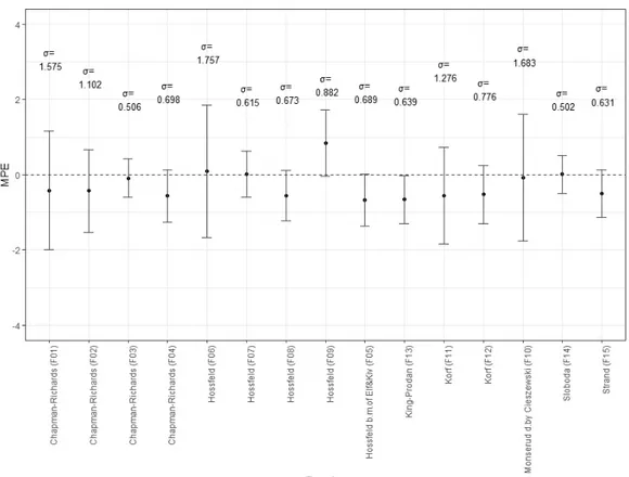
Out of fifteen tested GADA equations, those based on base equations of exponential form showed the best fit. The parameter estimates for each model and their fit and prediction statistics are summarized in Table 6. All parameters, except parameter b2 and b3 of model F13, were found to be significant at 1% level. Models showed different goodness-of-fit statistics, varying from very good fit, shown by models developed using equations F01, F02 and F14, to mediocre and even rather poor fit. Based on the graphical appearance of models (Appendix 1.), most of the models showed poor ability to follow and encompass the actual growth pattern of measured trees. Models F02; F03; F05; F08 and F14 had the best visual conformity with the measured data, but models F03 and F14 were identified as superior ones. Both, model F03 (developed using Chapman-Richards base model) and F14 (developed using Sloboda base model) showed very good fit statistics and had the best prediction statistics, i.e. Chapman-Richards model and Sloboda model had the smallest mean prediction error (MPE) and smallest standard deviation (σ) within the predicted values, when predicting height at both 15 (Fig. 7) and 10 years (Fig. 8) of age.

(31)

29

Figure 7. Mean prediction error (MPE) for height predictions at the age of 15 years.

(32)

30

Considering the superior performance of models F03 and F14 in every aspect evaluated, the following results will focus on only these two models. Both models outperformed other candidate models when their accuracy to predict the height of individual trees was tested. All models were tested by their ability to predict height at the age of 10 and at the age of 15 years using different starting heights at different reference ages. For most of the models, including Chapman-Richards and Sloboda model, prediction errors increased with an increasing difference in age between the starting height and predicted height, i.e. the younger the tree, the larger the error when predicting its height at later age. Chapman-Richards and Sloboda model (Fig. 9 & 10) both had the largest MPE (-0.345 m and -0.232 m respectively) when predicting height from 6 years of age. Contrary to Chapman-Richards model, Sloboda model showed higher accuracy in predicting height at the age of 15 years. As the age difference between the starting height and predicted height decreased, Chapman-Richards model showed more stability and thus higher precision compared to Sloboda model which showed more fluctuating predictions.

(33)

31

(34)

32 T a b le 6 . P ar am et er es ti m at es an d f it s ta tis tic s o f mo d els u se d in th is s tu d y M ode l F it s ta ti st ic s P re d ic ti o n s ta tis ti cs P ar am . Es t. SE t p > t M P E1 0 M P E1 5 S D1 0 S D1 5 R M S E1 0 R M S E1 5 A IC F0 1 b2 0.0644 0.0013 48.31 2*10 -16 -0.383 -0.42 0.663 1.575 0.7650 1.6296 35 583 b3 2.5979 0.0164 158.18 2*10 -16 F0 2 b1 14.7232 0.0897 164.0 2*10 -16 0.049 -0.432 0.482 0.698 0.4950 0.8939 24 398 b3 3.9272 0.0198 198.2 2*10 -16 F0 3 b1 19.23 0.1368 140.6 2*10 -16 -0.117 -0.095 0.393 0.506 0.4099 0.5148 14 208 b2 0.1062 7.421*10 -4 143.1 2*10 -16 F0 4 b1 0.1646 0.0014 109.90 2*10 -16 -0.114 -0.559 0.568 1.102 0.5695 1.1828 28 170 b2 7.563 0.0704 107.37 2*10 -16 b3 -0.1857 0.0022 -81.72 2*10 -16 F0 5 b2 -2.825 7.606*10 -3 -371.4 2*10 -16 -0.089 -0.676 0.516 0.689 0.5231 0.9652 3 3 723 be ta 1.191*10 +3 8.661 137.5 2*10 -16 F0 6 b1 2.392*10 +7 4.466*10 +4 535.5 2*10 -16 -0.488 0.094 0.644 1.757 0.8243 1.7590 47 714 b2 3.119*10 +7 6.263*10 +4 498.0 2*10 -16 b3 1.918 2.202*10 -3 871.3 2*10 -16 F0 7 b1 10.8145 0.0357 3 02.81 2*10 -16 -0.183 0.017 0.438 0.615 0.4744 0.6248 17 264 b2 124.6595 2.8380 43.92 2*10 -16 b3 -2.5256 0.0069 -361.2 2*10 -16 F0 8 b1 14.1449 0.0743 190.2 2*10 -16 -0.077 -0.557 0.509 0.673 0.5143 0.8864 24 215 b3 2.8098 0.0068 410.7 2*1 0 -16 F0 9 b1 0.09443 5.434*10 -4 173.8 2*10 -16 -0.941 0.845 0.647 0.882 1.1418 1.0851 40 901 b2 -0.06473 9.469*10 -5 -683.6 2*10 -16 F1 0 b1 9.655*10 +3 1.435*10 +3 6.73 1.76*10 -11 -0.611 -0.087 0.615 1.683 0.8664 1.6844 47 340 b2 0.9701 1.629 *10 -3 595.63 2*10 -16 b3 1.998 4.806*10 -3 415.86 2*10 -16 y0 -8.332*10 +3 4.461*10 +2 -18.68 2*10 -16 F1 1 b1 0.0697 0.0110 6.326 2.59*10 -10 -0.303 -0.556 0.579 1.276 0.6536 1.3916 31 984

(35)

33 T a b le 6 ( cont inue d) N o te : P a ra m . is p ar a m et er , E st . is es ti m at ed v al u e o f t h e p ar a m et er , SE i s st a n d ard e rro r, M P E is m ea n p re d ic tio n e rr o r, SD is s ta d ar d d ev ia tio n a n d R M SE is r o o t m ea n sq ua re d e rro r. M ode ls F it s ta ti st ic s P re d ic ti o n s ta tis ti cs P ar am . Es t. SE t p > t M P E1 0 M P E1 5 S D1 0 S D1 5 R M S E1 0 R M S E1 5 A IC b2 54.8724 0.7035 77.995 2*10 -16 b3 0.5018 0.0070 70.958 2*10 -16 F1 2 b1 57.4726 1.2965 44.33 2*10 -16 -0.179 -0.521 0.453 0.776 0.4867 0.9347 25 565 b3 0.7004 0.0057 121.99 2*10 -16 F1 3 b1 2.879 7.197*10 -3 400.03 2*10 -16 -0.059 -0.656 0.5 0.639 0.5030 0.9157 32 219 b2 -4.511*10 +6 2.46*10 +8 -0.183 0.854 b3 6.002*10 +7 3.273*10 +8 0.183 0.854 F1 4 b1 54.8724 0.1088 147.53 4 2*10 -16 -0.121 0.01 0.390 0.502 0.4085 0.5018 12 180 b2 0.5018 0.0025 68.72 2*10 -16 b3 57.4726 0.0082 4.787 1.71*10 -6 F1 5 b1 0.7004 2.095*10 -3 561.63 2*10 -16 0.148 -0.495 0.465 0.631 0.4878 0.8017 26 707 b2 2.879 4.471*10 -4 -58.22 2* 10 -16 b3 -4.511*10 +6 0.1902 -89.32 2*10 -16