Linkage between FinTech and Traditional Financial Sector in U.S. : Comparative Study during and after Global Financial Crisis

Linkage between

FinTech and

Traditional Financial

Sector in U.S.

MASTER THESIS WITHIN: Business Administration in Finance

NUMBER OF CREDITS: 15 credits

PROGRAMME OF STUDY: International Financial Analysis

AUTHOR: Chunyan Chen, Ziyi Zhang

JÖNKÖPING: May 2018

——Comparative Study during and after Global

Financial Crisis

Acknowledgements

Foremost, we would like to express our sincere gratitude to our advisor Prof. Andreas Stephan for the useful comments, remarks and engagement through the learning process of this master thesis, He is always willing to help us whenever we ran into a trouble or

encountered problems about our research or writing, his guidance helped us in all the time of this thesis.

Furthermore, we also grateful to the students of our seminar group for their discussions. Their constructive opinions have allowed us to constantly improve this article.

Most importantly, none of this could have happened without our family. Thanks for their unconditional love and encouragement through past few months.

Jönköping International Business School, May 2018

______________________________ _______________________________

Master Thesis in Business Administration

Title: Linkage between FinTech and Traditional Financial Sector in U.S.

——Comparative Study during and after Global Financial Crisis

Authors: Chunyan Chen and Ziyi Zhang Tutor: Andreas Stephan

Date: 2018-05-15

Key words: Fintech, Traditional financial sector, Granger causality, Toda&Yamamoto, linkage

Abstract

Background: In 2008, the financial crisis led to the deterioration of the global economy. The financial industry suffered severe setbacks. On the one hand, regulators strengthened their supervision over financial institutions and raised capital requirements. On the other hand, publics’ confidence in financial institutions declined. At the same time, the fintech industry has rapidly developed during this decade, they use technology to make financial innovation and pose a threat to the traditional financial industry.

Purpose: This paper aims to study the linkage between U.S. fintech and the traditional financial sector, trying to figure out which industry's stock price changes will affect the stock price changes in another industry. In particular, it also considers whether the global financial crisis will affect this relationship.

Method: We first perform the Granger causality test under the VAR framework for several selected indices sequences, and then use the Toda Yamamoto version of Granger causality approach to verify the reliability of the above tests. Testing is divided into different time intervals in order to detect the impact of financial crisis on the relationship between time series. Conclusion: The empirical analysis results show that the correlation between the index in the long-term and short-term is inconsistent, and also shows that the correlation between the

Table of Contents

1.

Introduction ... 1

2.

Fintech profile ... 4

2.1.1 New payment methods ... 5

2.1.2 Diversified financing methods ... 5

2.1.3 Smart asset management services ... 6

2.1.4 Other fintech sectors ... 6

2.2 Fintech evolution ... 7

2.3 Fintech in United States ... 8

3.

Literature review ... 8

3.1 Fintech and traditional financial sector ... 8

3.2 Global financial crisis affects relationship between Fintech and traditional financial sector... 10

3.3 Granger causality and Toda&Yamamoto ... 11

4.

Data description ... 12

5.

Methodology ... 13

5.1 Augmented Dickey-Fuller (ADF) Test ... 14

5.2. Johansen Test ... 17

5.2 Granger Causality Test ... 19

5.3 Toda Yamamoto Granger Causality ... 20

6.

Empirical results ... 21

6.1 Full sample analysis ... 21

6.1.1 Autocorrelation and inverse roots ... 24

6.1.2 Granger causality Test for full sample period ... 24

6.1.3 Toda Yamamoto Granger Causality Test for full sample period ... 25

6.2 Sub-period analysis ... 28

6.2.1 Granger Causality Test for sub-sample periods ... 31

6.2.2 Toda Yamamoto Granger Causality Test for sub-sample period ... 34

7.

Conclusions ... 36

8.

Discussion ... 37

9.

References ... 38

Appendix ... 41

Crisis-period ... 43

Autocorrelation test or crisis period ... 43

AR Roots Graph for crisis period: ... 44

Post-crisis ... 46

Autocorrelation for post-crisis period ... 46

AR Roots Graph for post-crisis period ... 47

Tables

Table 2: Decriptive statistics and correlation matrix for full sample period...21

Table 3: Augmented Dickey–Fuller (ADF) Test for full sample period...23

Table 4: Granger Causality Test for full sample period...24

Table 5: Johansen's cointegration Test for full sample period...26

Table 6: Toda Yamamoto Granger Causality Test for full sample period...27

Table 7: Descriptive statistic and correlation matrix during the crisis period...29

Table 8: Descriptive statistic and correlation matrix during post-crisis period...29

Table 9: Augmented Dickey–Fuller (ADF) Test for sub-sample period...31

Table 10: Granger Causality Test for sub-sample period...32

Table 11: Johansen's cointegration Test sub-sample period...34

1. Introduction

The term “fintech” which is the abbreviated form of financial technology, In March 2016, the International Financial Stability Board (FSB) released its first special report on financial technology, initially defining the term "financial technology." In other words, fintech refers to financial innovation brought about by technology. It can create new business models, processes, applications or products that may have a significant impact on the way financial markets, financial institutions, or financial services are provided. The narrow sense of financial technology refers to the non-financial institutions can reshape traditional financial products, services, and organizations by using mobile Internet, cloud computing, and big data (Bernardo, 2017). Financial technology is broadly defined as the application of technological innovation in the field of financial services. Financial technology has also been defined as a company that combine financial services with modern, innovative technologies, fintechs are typically attract customers with more user-friendly, efficient, transparent, and automated products and services than those currently available (Gregor, Lars, Matthias, & Martina, 2017).

1.1 Background

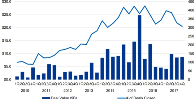
According to a report issued by KPMG in February 13, 2018, the global fintech sector received nearly 25 billion US dollars investment in the fourth quarter of 2015, which is the highest investment quota in history, while the United States received most of the investment, nearly 18 billion U.S. dollars. On the other hand, statistics from the Federal Deposit Insurance Corporation (FDIC) shows that in the 2015, 42.1 percent of households earning less than $30,000 per year were unbanked or underbanked. The reason for households for being unbanked is mainly because many of them think that banks are not interested in serving families like them. Consumers who do not trust banks or feel banks are not interested in addressing their needs are unlikely to consider banks as an option to meet their financial needs.

Table 1: Global investment activity (VC,PE and M&A) in fintech companies

Source: (KPMG, 2018)

For many reasons, the financial institutions were regarded by public as the main culprit behind the 2008 financial crisis: banks and financial institutions have suffered huge losses during the financial crisis; customers have become increasingly distrustful of financial institutions; and in order to consider individual contributions to global risk, the Basel Committee on Banking Supervision (BCBS) has increased banks’ regulatory reserve requirement; Benoit et al. (2016) Similarly, regulators required many companies to verify and improve their solvency. Such political and economic environment has increased the opportunities and promoted the development for technology-based companies.

After 2008 financial crisis, fintech sector has developed rapidly over the past decade and is considered as one of the main disruptors of traditional financial services. whether it is to provided new ways to enhance the customer experience or improve the efficiency of back-office functions – fintech solutions are reshaping the financial service industry. Fintech covers the overlapping area of technology and financial services. The digital revolution, the popularity of smartphones and internet, making customers more comfortable and relying on technology-based financial solutions. Fintech has penetrated into every aspect of people's lives. Nowadays, some prominent fintech companies are vying for market share with traditional banks since the fintech companies can provide convenient loans, transfers and investment methods with lower service costs, more open lending standrads and more personalized services.

According to Statiscal's data, in the past decade, fintech has expanded its services to different business areas. Financial technology companies with payment services are the most attractive investment objects in the financial technology sector, obtained 70% of total amount in the fintech investment in 2013. A KPMG report also shows that although the payments and leding companies are still highly attractive to U.S. investment, the insurtech is gain more attention among investors in 2017.

Traditional financial banks and institutions have many loyal customers due to well-entrenched banking system and resonable services to the mass market. However, traditional financial institutions are losing their advantages since fintech startups can offer more customer-centric products and services. Fintech startups can use advanced technology to provide more affordable, more personalized services, and make services more efficient and build closer relationships with customers.

1.2 Purpose

In the stock market, fluctuations between industries have a chain effect. Volatility of an industry often leads to fluctuations in another industry. As an emerging industry that has developed over the past decade, fintech has brought new challenges to the traditional financial industry, the linkage between the traditional financial sector and fintech sector is worth to study. After a large number of previous studies, we found that the emergence of financial crisis and the choice of different time intervals will affect the relationship between stocks.

The main purpose of this paper is trying to figure out the co-movement relations between fintech sector and traditional financial institutions by analyzing the changes in U.S. financial services indices and fintech index over time from 2007 to 2016. Then, we compare the sample data during the financial crisis and after the financial crisis to discuss whether the financial crisis will affect the linkage between the two industries. Ultimately, we hope that investors can realize the fluctuations and volatility between those two industries and improve their ability to avoid risks.

1.3 Problem statement

As most researchers have said, financial technology is changing the pattern of the traditional financial industry. It is usually more interesting to study which side caused the causality of the other party than to simply study the connection between the two variables.

What are we interested is that under such market trend, the causal relationship between fintech and traditional financial industry is from which side to the other party. We also noticed that the relationship between stocks is not constant, but will change under certain special market conditions or at different time intervals. Therefore, we also focus on the relationship between fintech and finance under different market conditions.

1.4 Perspective

This paper adopted the Granger causality VAR, and Toda & Yamamoto method of Granger Causality to study the linkage between the traditional financial sector and the fintech sector during the financial crisis and after the financial crisis in the U.S. market. Most previous studies have focused on the linkage between these two, while only a few have conducted comparative studies on this connection. Therefore, from the perspective of investors, we compared the linkage between fintech and traditional financial sector in the United States in different periods. Fintech is a new and dynamic field and hopes that this study will provide investors with a prudent view of fintech and realize the impact of the different market condition on the stock market.

1.5 Delimitation

There are many overlapping businesses in the traditional financial and fintech fields, such as investment, and asset management, etc. However, we only selected the banking index and the insurance index that are most closely related to the fintech, we did not consider other parts in our research. Secondly, due to the available data in fintech sector in other countries are difficult to obtain, we only studied the U.S. market. Finally, different market conditions will lead to different empirical results, therefore, this article does not have horizontal comparisons to present a more complete perspective. Moreover, we adopted the daily data to study the relationship among these series, however, such high frequency data will yield the different results compared with weekly and monthly data, this should be considered in the further study.

In this section, we will briefly introduce fintech's basic nature, development status, and the links with the traditional financial institutions, so as to help readers have a basic understanding of fintech.

2.1 Fintech segment

Fintech is divided into six categories which are payment, wealth management, crowdfunding, lending, capital market, and insurance services (In & Yong Jae, 2018) . Simultaneously, fintech also is classified into four major segments, which are financing segment, asset management segment, payments (Gregor, Lars, Matthias, & Martina, 2017). Similarly, here we divided the fintech industry into four categories, and the definition of those segments are described below.

2.1.1 New payment methods

Mobile payments allow payment activities available through portable electronic devices. With the advancement of information technology, more traditional payment services have been replaced by new payment methods. There are already several payment methods, such as SMS/USSD-based transactional payments, mobile web payments, QR code payments, NFC near field payments, and biometric technology payments.

Payments sector also includes blockchain and cryptocurrency (Michael, Peter, Oliver, & Dirk, 2017), who describe that the blockchain is usually extended by each additional block, thus representing a complete ledger of the transaction history. Each block contains a timestamp, a cryptographic hash of the previous block, and transaction data. The most well-know application of blockchain technology is the cryptocurrency. Each transaction history is stored into the peer-to-peer network of Bitcoin, making it difficult to forge informaiton (Grinberg, 2011).

The digitalization of the financial industry has caused the payment value chain to suffer, and the traditional incumbents have been affected by the emerging fintech companies. (Claudio, 2017)

2.1.2 Diversified financing methods

The traditional financing methods has insufficient financing channels and often associated with high financing costs, which makes it difficult for many small businesses and individuals to obtain financing. With the development of e-commerce, payment

technologies, and big data technology, the way of financing has also changed along with it. Crowdfunding is a new platform enables entrepreneurs to raise money from anyone who is interested in investing in their projects, crowdfunding is based on the participation of a large number of “investors” who provide the financial resources to achieve the same goal. Due to different financing purpose, crowdfunding is divided into four different types, which are donation-based crowdfunding, reward-based crowdfunding, crowd investing, and crowd lending.

Some fintech startups extend credit to individuals and small businesses by cooperation with partner banks, loans can generally be delivered via mobile phones in a short period of time. Fintech also provides new factoring solutions like online sales claims or no-frills solution (Gregor, Lars, Matthias, & Martina, 2017).

2.1.3 Smart asset management services

Bag data, cloud computing, and artificial intelligence technology have developed rapidly in the past decade. These technologies have been applied to the financial sector and provide clients with investment advices and consulting. Smart investment consultants are more rational, precise, and efficient than traditional ones, it also has lower costs. The current innovation of intelligent asset management services mainly includes the use of artificial intelligences algorithms in investment decisions, the application of big data and automation technologies in information collection and processing, the use of human-computer interaction techniques in determining investment objectives and risk control processes, as well as the application of cloud computing in improving the application management and risk management.

2.1.4 Other fintech sectors

There also has other fintech sectors offer services beyond traditional banks function. Insurtech is a combination of insurance and technology, insurtech is more efficient and save more costs than current insurance industry, it can be used to collect and analyze customer data to provide better services. According to Accenture, the total value of deals in North America accounting for US$ 1.24 billion in 2017, smartphones apps, online policy handling, claims processing, wearables, and automated processing are all insurtech. Insurtech is disrupting the insurance sector. Other fintech startups also provides technical solutions for financial services provider like traditional banks.

2.2 Fintech evolution

The development of financial technology has a history of 150 years so far, there are three major stages of development. From the 1866 to 1967 (Arner, Barberis, & Buckley, 2016) (Bernardo, 2017) , finance and technology were interrelated and mutually promoted. Technologies such as steamships, railways and telegraphs laid the foundation for cross-border financial interconnection in the late 19th century. After the First World War, finance and technology developed rapidly, the global telex network provided the guarantees for the development of the next phase of financial technology, this is the era of fintech 1.0.

The following period from 1967 to 2008 is so-called fintech 2.0, in early 1970s, the US Clearing House Interbank Payment system established, The United States begins to establish an automated electronic communication system, and the Fed’s member banks use Fedwire to provide services. In 1995, Wells Fargo started to offer online consumer banking. In 2001, eight banks of the United States had at least one million customers online. In the late 1990s, the Internet opened the door to the rapid development of financial technology after 10 years.

Fintech 3.0 began at 2008, the global financial crisis damaged the bank's brand image. Banks and financial institutions not only suffered huge losses during this period, but also the trust of customers in banks and financial institutions declined significantly. On the other hand, the Basel Committee on Banking Supervision (BCBS) has also increased the bank's regulatory reserve requirements to consider individual contributions to global risk (Benoit et al. 2016). According to Federal Deposit Insurance Corporation (FDIC), in the 2015, 27 percent of households in the united states are unbanked or underbanked, and 42.1 percent of households earning less than $30,000 per year were unbanked or underbanked. The reasons for households for being unbanked are mainly because many of them feels that banks have no interest to serving households like theirs, Consumers who either do not trust banks or feel banks are not interested in addressing their needs are unlikely to see banks as an option to meet their financial needs, in another survey in 2015, Americans were more willing to let technology companies manage their assets than banks. In the era of financial technology 3.0, part of the financial services of banks was gradually replaced by financial technology startups. In addition, financial technology startup

companies have grown faster than traditional financial services industries and can provide customers with more personalized services. This change has emerged from the global financial crisis in 2008, and technology companies have penetrated into the financial industry and a diversified banking system.

2.3 Fintech in United States

The revolution in financial technology innovation has driven the global traditional financial industry into a new stage. While the United States is at the forefront of this revolution, the financial innovation of the United States is dominated by the financial hubs of the country, through financial market participants (banks, institutional investors, Insurance companies, etc.) nurturing and funding (Julapa & Catharine, 2018).

According to the report of KPMG (2015), the global financial technology investment amounted to 20 billion U.S. dollars, and the investment amount in the three years increased by about seven-fold. Another report (CB Insights & KPMG, 2015) pointed out that in 2015, North America is the leader in this funding, nearly all of the 7.7 billion U.S. dollars was raised in the US. The United States is the most critical market in the world, and more and more fintech companies have achieved success in the United States, such as LendingClub, Plaid, Kensho, etc.

3. Literature review

3.1 Fintech and traditional financial sector

"FinTech," a contraction of 'financial technology," refers to technology enabled financial solutions (DOUGLAS, JANOS, & Ross, 2016). It is also seen as a combination of financial services and information technology.However, the initial link between finance and technology can be traced back to 1866. (Barbiroli, 1997) The Automatic Teller Machine (ATM) first introduced by Barclays Bank in 1967 can be regarded as the symbol of the beginning of the development of modern financial technology (Thomas , 2013). Then, in the latter part of the 20th century, the financial digitization process achieved rapid development. Since the late 1980s, the financial industry has been relying on digital information for its operation and transmission. By the mid-1990s, the financial services industry had become the largest single buyer in the digital information industry and

continued to this day (OLIVER , 2015). Therefore, the traditional financial industry has driven the IT industry for at least two decades, and due to the rise of fintech in recent years, IT spending in the future financial industry is expected to more than double (Elliott , 2015). Finally, since 2008, in the third era of fintech development, emerging fintech companies have perfectly integrated finance and technology, and some of them can directly provide financial products and services to enterprises and the public.Therefore, fintech has emerged in developing countries and grown rapidly.

The rapid rise of Fintech has affected the business environment of the traditional financial industry, which has led the banking industry to seek more innovative ways of operation, such as increasing investment in fintech (Inna & Marina, 2016). Inna and Marina give a detailed analysis of the development of Fintech and banking in Europe and the United States between 2008 and 2015. They draw a conclusion that there is a unilateral relationshipbetween the banking industry and fintech in the global financial crisis and no mutual influence after the global financial crisis. It shows that when facing the upsurge of fintech, the banking industry should strengthen financial innovation and effectively control its risk.

Some people in the financial industry regard the existence of fintech as a threat to traditional financial industry, while others see the rise of fintech as a challenge and an opportunity to improve the financial business. The relationship between the emerging fintech digital bank and the financial industry has been studied by Yinqiao, Renée, & Laurens (2017) , theyprobed into the impact of the stock returns of 47 American retail Banks from 2010 to 2017, then obtain that the growth of fintech's funds is positively correlated with the stock returns of existing retail Banks, indicating that there is complementarity between fintech and traditional Banks (Yinqiao, Renée, & Laurens, 2017). Sabine, Nicole, Shan, & Susanne (2018) open up another new way for us to study the relationship between fintech and the traditional financial industry - Insurtech, like fintech, is one of the fastest growing emerging industries in recent years. They explained the meaning of insurtech in detail and discussed the development process and future trends of insurtech in depth (Sabine, Nicole, Shan, & Susanne, 2018). In short, fintech is closely related to the traditional financial industry. It not only integrates the traditional

financial industry and information technology, but also determines the direction of the traditional financial industry to some extent.

3.2 Global financial crisis affects relationship between Fintech and traditional financial sector

In 2008, with the collapse of Lehman Brothers in New York, the financial institutions of the world suffered a large-scale collapse and the global financial market began to turmoil. The global financial crisis in 2008 has had a great impact among the world. Although this financial crisis has worsened public opinion on financial institutions, banks, and financial services practitioners (Sumit, Gene, & Itzhak, 2014), on the other hand, it has brought fintech into the public’s perspective, which not only enables financial professionals to find new and promising industries to use their skills (Mark & Terence , 2014), but also provides a new platform for fresh graduates, new generations, and ordinary people who pay attention to finance (Quentin, 2014).

The deterioration of public perception has hindered the development of the traditional financial industry to some extent in the United States. Predatory loans would not only make citizens think that their rights and status have been threatened, but also violate the bank’s obligations to protect consumers (Sumit, Gene, & Itzhak, 2014). And the severe financial crisis in the latter turned into the economic crisis had led up to 8.7 million American workers unemployed (John, 2014). Many financial practitioners also encountered the problem of insufficient compensation or unemployment during this financial crisis.The depressed employment prospects and the public’s distrust to financial institutions, making them lost confidence in the traditional financial industry (Mark & Terence , 2014).

The global financial crisis in 2008 played a role in the rise and development of fintech. Many customers in the financial services industry, especially the young generation, have lost confidence in the traditional financial industry after the financial crisis. They may think that traditional financial institutions are a source of financial and economic crisis, and therefore are more willing to see emerging companies like Fintech companies are not involved in the recent crisis, which means innovative solutions may be offered to customers.Therefore, Bernardo conducts some research and analysis on the impact of the

2008 financial crisis on the relationship between fintech and the traditional financial industry and find that the financial crisis has deepened the relationship between fintech and the financial industry (Bernardo , 2017). According to Yonghong, Shabir, and Mengmeng’s (2017) study, the vector auto-regression (VAR) model was used to conduct the Granger causality tests, to discusses the impact of the pre-, mid- and post-crisis periods on the six major stock markets of the United States, the United Kingdom, Germany, Hong Kong, mainland China, and Japan. The interdependence relationship between the six major stock markets was obtained, which shows that comparing with before and after the global financial crisis, the relationship between the six major stock markets became much closer when the financial crisis occurred (Yonghong, Shabir, & Mengmeng, 2017).

With the development of technology, fintech has become a new engine for the development of the economy of the world. During the financial crisis, fintech can make up for the market mechanism and form a new market mechanism together with traditional finance. Li & Zhang (2009) conclude that the global financial crisis has a certain influence on the causal relationship between fintech and the traditional financial industry, which maybe represents that the participation of fintech can partly resist the damage caused by the financial turmoil (Li & Zhang, 2009).

3.3 Granger causality and Toda&Yamamoto

Use ordinary granger causality test to examine the relationship between fintech and traditional financial industry. Toda & Yamamoto approach is also tested to avoid the problems of power and size properties of unit root and cointegration tests in normal Granger causality test and double check the results (Nicholas & James , 2009).

Zeynel, Hasan & Bedriye (2008) used the method of granger causality test to examine the dynamic linkages between the United States central stock market and emerging stock markets, such as fintech, from the date reported to 24th March 2006, which indicates that the existence of unilateral causality from S&P500 to the stock prices of the 15 emerging markets (Zeynel, Hasan, & Bedriye, 2008). Rizwan, Jolita & Dalia (2017) aim to explore the long-term relationship between stock returns of the KSE100 index and some monetary indicators between 1992 and 2015. After using the augmented Dickey–Fuller (ADF) method and Johansen cointegration approach, the Grander causality test and Toda and

Yamamoto procedure proved that unilateral causality exists from the interest rate to KSE100 index (Rizwan, Jolita, & Dalia, 2017). Chien-Chiang, Wei-Ling & Chun-Hao (2013) used the method of Granger causality test of Toda and Yamamoto to discusses the lead-lag relationship and dynamic relationship between the stocks, insurance and bond markets in six developed countries, including Canada, the United States, the United Kingdom, France, Italy, and Japan, from 1979 to 2007.Their results show that although the direction is different, there is dynamic relationship between countries.(Chien-Chiang, Wei-Ling, & Chun-Hao, 2013) Test the dynamic correlation of the stock returns of six leading stock markets of South America, augmented Dickey-Fuller (ADF) test, Phillips-Perron (PP) test, and Kwiatkowski-Phillips-Schmidt-Shin (KPSS) tests techniques are used to test the unit root of the variables, Box-Pierce statistics and Ljung-Box Q-statistic are used for testing stationarity of variables, Ajaya & Swagatika (2018) mentioned that the Classical Linear Regression Model is not suitable for financial time series, since the model is assuming that the variance of the error term is constant, but real world data of financials are typically inconsistent. (Ajaya & Swagatika, 2018) All these literatures provide inspiration and guidance for exercising the test in our article.

4. Data description

The data used in the following test are KBW Financial Technology Index (KFTX), S&P Financial Services Select Sector Index, S&P 500 Banks Index and S&P 500 Insurance Index respectively. Many branches of the financial services sector have been affected by fintech, but we learned from many previous literatures that banking sector are most affected by fintech, and that insurance has also been affected in recent years with the development of insurtech. Thus, we particularly choose these two sectors to examine the impact of fintech.

The data was obtained from Thomson Reuters DataStream and NASDAQ GLOBAL INDEX ranges from 3 January 2007 to 9 February 2016, yielding a total of 2292 daily observations for each index.

According to NASDAQ GLOBAL INDEX, the KBW Financial Technology Index (KFTX) is designed to precisely track the performance of fintech companies that are publicly traded in the United States. KFTX index includes 49 fintech companies which

leverage technology to delivery financial products and services. Index selection is not limited to securities within a particular industry classification due to the fact that the fintech is a young field and fintech companies are not easily categorized in to a single industry group. KFTX index covers business areas such as payments, credit cards, banks, credit scoring, trading exchanges and more, major components included in such as PayPal Holding Inc., Visa Inc., and LendingClub Crop. The S&P Financial Services Select Sector includes 69 companies from financials sectors excluding Real Estate but keeping Mortgage REITS, both S&P 500 BANKS INDEX and S&P 500 INSURANCE INDEX are sub-index of S&P 500 index, which reflects the trend of stock prices in each industry. The analysis was conducted by using continuously-compounded daily return, all the indices was calculated in the form of natural log difference as following equation:

𝑅𝑅𝑡𝑡=ln (_𝑃𝑃𝑃𝑃_𝑡𝑡−1𝑡𝑡 ) =ln (𝑃𝑃𝑡𝑡)-ln (𝑃𝑃𝑡𝑡−1)

Where 𝑅𝑅_𝑡𝑡 is regarded as the index return of each index at period of time t, 𝑃𝑃_𝑡𝑡 and 𝑃𝑃_𝑡𝑡−1 are the closing price for the current day t and previous daytime period t-1.

In order to detect the effects of global financial crisis on the relationship of each pairwise indices, the sub period analysis is conducted after the full sample period analysis, the first period starting form 3 January 2007, which is suggested by (Covitz, Liang, & Suarez, 2013) and (Polanco-Martínez, Fernández-Macho, Neumann, & Faria, 2018) to including it in the sub-period during the financial crisis, the second period from 3 January 2011 to 9 February 2016 is referred to as post-crisis period.

5. Methodology

The following is a brief introduction of the main method used in this paper: 5.1 Augmented Dickey-Fuller (ADF) Test

Augmented Dickey-Fuller (ADF) test was firstly applied to each index, this formal test is known as unit root test of random walk series or say, non-stationary. The existence of a unit root has been used as the null hypothesis, which means that the ADF test is based on the assumption that the error terms are identically distributed and independently. But the shortcoming of ADF test is if adding the lagged difference terms of the regressand it may suffer with serial correlation in the error terms. Brooks (2008) states that non-stationarity can lead to unreliable estimation and spurious correlation, that is the reason why Unit root test with Augmented Dickey-Fuller (ADF) test is the first step for each variable to ensure the time-series data we used are stationary.

The general ADF inspection is divided into 3 steps:

Data

properties

•Augmented Dickey-Fuller(ADF) test is initially applied to

Causality

•Autocorrelation: which is a common procedure to time-series data in order to see wether the error terms are correlated. •Granger causality test: To detect the causal relationship among

series.

Robust test

•Johansen Cointegration Test is adopted to check the long-run relationship of variables.

•Toda Yamamoto Granger Causality Test: Due to the advantages of this test, we use it to verify the results of traditional Granger Caulity Test, and strengthen the reliability of our results

a.Test the original time series. At this time, the second item is selected as the level and the third item is None. If the item fails the test, the original time series is not stable; b.Perform a first-order differential test on the original time series, that is, select the 1st difference in the second term and the interception in the third term. If it still fails the test, you need to perform a second difference transformation;

c.The test of the second differential sequence, that is, the second choice 2nd difference, the fourth choice Trend and intercept. Generally this time series is stable!

The relevant formula involved is as follows,Let's consider a model first: 𝑌𝑌𝑡𝑡= 𝜌𝜌𝑌𝑌𝑡𝑡−1+ 𝑢𝑢𝑡𝑡

Where Ut is the random noise term for white noise, we can get the following three formulas from this model:

𝑌𝑌𝑡𝑡−1= 𝜌𝜌𝑌𝑌𝑡𝑡−2+ 𝑢𝑢𝑡𝑡−1 𝑌𝑌𝑡𝑡−2= 𝜌𝜌𝑌𝑌𝑡𝑡−3+ 𝑢𝑢𝑡𝑡−2 𝑌𝑌𝑡𝑡−𝑇𝑇 = 𝜌𝜌𝑌𝑌𝑡𝑡−𝑇𝑇−1+ 𝑢𝑢𝑡𝑡−𝑇𝑇

By bringing the three formulas into the adjacent formula one by one, you can draw: 𝑌𝑌𝑡𝑡= 𝜌𝜌𝑇𝑇𝑌𝑌𝑡𝑡−𝑇𝑇+ 𝜌𝜌𝑢𝑢𝑡𝑡−1+ 𝜌𝜌2𝑢𝑢𝑡𝑡−2+ ⋯ + 𝜌𝜌𝑇𝑇𝑢𝑢𝑡𝑡−𝑇𝑇+ 𝑢𝑢𝑡𝑡

According to the different values of ρ, it can be considered in three situations:

1. If ρ < 1, then when T → ∞, 𝜌𝜌𝑇𝑇 _{→ 0, that is, the impact on the sequence will gradually} weaken with time, and the sequence is stable.

2. If ρ > 1, then when T → ∞, ρ → ∞, that is, the impact on the sequence over time will gradually increase. It is clear that the sequence is unstable at this time.

3. If ρ=1, then when T→∞, ρ=1, that is, the impact on the sequence is constant over time. Obviously, the sequence is also unstable.

For the original model, the ADF test is equivalent to the significance test of its coefficient. The established null hypothesis is: 𝐻𝐻₀: ρ =1. If we reject the null hypothesis, we say that 𝑌𝑌𝑡𝑡 has no unit root. At this time, 𝑌𝑌𝑡𝑡 is stationary. If we cannot reject the null hypothesis, we say that 𝑌𝑌_𝑡𝑡 has a unit root. At this time, 𝑌𝑌_𝑡𝑡 is called the random walk sequence is unstable.

The original model can also be expressed as:

Δ𝑌𝑌𝑡𝑡= β1+ β1𝑡𝑡 + 𝛿𝛿Yt−1+ 𝛼𝛼i� 𝛥𝛥Yt−i 𝑚𝑚 𝑖𝑖=1

+ Ut

Among them, where Δ𝑌𝑌_𝑡𝑡 = Y_t-Y_t−1, Δ is a first-order difference operation factor. The null hypothesis at this time becomes: 𝐻𝐻₀: ρ=0. Note that if 𝐻𝐻₀ cannot be rejected, then Δ𝑌𝑌_𝑡𝑡=U_t is a stationary sequence, that is, Y_t's first-order difference is followed by a stationary sequence. At this time, we call a sequence of first-order single integer processes, denoted as I (1). The I(1) process is the most common in financial and economic time series data, while I(0) represents a stationary time series.

From the perspective of theory and application, the inspection model of ADF test has the following three:

𝑌𝑌𝑡𝑡 = (1 + 𝛿𝛿)Yt−1+ Ut which is Δ𝑌𝑌𝑡𝑡 = 𝛿𝛿Yt−1+ Ut ① 𝑌𝑌𝑡𝑡 = 𝛽𝛽1+ (1 + 𝛿𝛿)Yt−1+ Ut which is Δ𝑌𝑌𝑡𝑡= 𝛽𝛽1+ 𝛿𝛿Yt−1+ Ut ② 𝑌𝑌𝑡𝑡= 𝛽𝛽1+ 𝛽𝛽2+ (1 + 𝛿𝛿)Yt−1+ Ut which is Δ𝑌𝑌𝑡𝑡 = 𝛽𝛽1+ 𝛽𝛽2+ 𝛿𝛿Yt−1+ Ut ③ Where t is the time or trend variable in each form, the established null hypothesis is 𝐻𝐻₀: ρ = 1 or 𝐻𝐻0: δ = 0, there is a unit root. The difference between ① and the other two regression models is whether it contains constants (intercepts) and trend terms.

After having the formula, we next determine the model. First, in order to comfirm whether the test model should contain constant terms and time trend terms. The empirical approach to solve this problem is examining data graphics. Second, we look at how to

judge the number of lag items m. In the empirical study, there are two commonly used methods:

a. Progressive t test. The method is to first select a large value of m, and then use the t test to determine whether the coefficient is significant. If it is significant, then choose the number of hysteresis items to be m; if it is not significant, reduce m until the corresponding coefficient value is significant.

b. Information guidelines. The commonly used information criteria are AIC Information Criterion and SC Information Criterion. In general, we choose to give the m value of the minimum information criterion value.

When dealing with non-stationary data, it is usually through the differential processing to eliminate the data of the non-stationary. That is, the time series is differentiated and then the differential series is regressed. After the first-order differential of financial data, that is, from total data to growth, it will generally be stable.

5.2. Johansen Test

In statistics, the Johansen test, is a procedure for testing cointegration of several, say k, I(1) time series. For the presence of I (2) variables (Johansen, Likelihood-based Inference in Cointegrated Vector Autoregressive Models, 1995). “Cointegration” is an attribute of two-time series data, two data sharing common stochastic drift. The benefit of Johansen Test is its capability of handle several time series variables. The Johansen Test is depending on Johansen's Trace Test and Maximum Eigenvalue Test.

In the VAR model, let 𝑌𝑌_1𝑡𝑡, 𝑌𝑌_2𝑡𝑡,..., 𝑌𝑌_{𝑘𝑘𝑡𝑡} be all non-stationary first-order single integer sequences, namely 𝑌𝑌_𝑡𝑡~I(1). 𝑋𝑋_𝑡𝑡 is an d-dimensional exogenous vector that represents a trend term, a constant term, etc.

𝑌𝑌𝑡𝑡 = 𝐴𝐴1𝑌𝑌𝑡𝑡−1+ 𝐴𝐴2𝑌𝑌𝑡𝑡−2+ ⋯ + 𝐴𝐴𝑝𝑝𝑌𝑌𝑡𝑡−𝑝𝑝+ 𝐵𝐵𝑥𝑥𝑡𝑡+ 𝜇𝜇𝑡𝑡

The first-order single integer process I(1) of the variables 𝑌𝑌_1𝑡𝑡, 𝑌𝑌_2𝑡𝑡,..., 𝑌𝑌_{𝑘𝑘𝑡𝑡} undergoes differential post-conversion to zero-order single integer process I(0)

𝛥𝛥𝑌𝑌𝑡𝑡= � 𝑌𝑌𝑡𝑡−1+ � Г_i 𝑝𝑝−1 𝑖𝑖=1 𝑦𝑦𝑡𝑡−𝑖𝑖+ 𝐵𝐵𝑥𝑥𝑡𝑡+ 𝜇𝜇𝑡𝑡 П_{= � 𝐴𝐴𝑖𝑖} 𝑝𝑝 𝑖𝑖=1 − 𝐼𝐼 Г 𝑖𝑖= − � 𝐴𝐴𝑗𝑗 𝑝𝑝 𝑗𝑗=𝑖𝑖+1

Among them, where 𝛥𝛥𝑌𝑌_𝑡𝑡 and 𝛥𝛥𝑌𝑌_{𝑡𝑡−𝑗𝑗} (j=1, 2, ..., p) are vectors composed of I(0) variables, and if 𝑦𝑦_𝑡𝑡−1 is a vector of I(0) (ie. 𝑦𝑦1_𝑡𝑡−1, 𝑦𝑦2_𝑡𝑡−1). There is a cointegration relationship between , ..., 𝑦𝑦𝑦𝑦_𝑡𝑡−1, then 𝛥𝛥𝑌𝑌_𝑡𝑡 is stable. According to whether the cointegration equation contains intercept and trend items, it is divided into five categories:

In the first category, the sequence 𝑦𝑦_𝑡𝑡 has no definite trend, and the cointegration equation has no intercept;

In the second category, the sequence 𝑦𝑦_𝑡𝑡 has no definite trend, and the cointegration equation has an interception term;

In the third category, the sequence 𝑦𝑦_𝑡𝑡 has a definite linear trend, and the cointegration equation only has an interception term;

In the fourth category, the sequence 𝑦𝑦_𝑡𝑡 has a definite linear trend, and the cointegration equation has a definite linear trend;

In the fifth category, the sequence 𝑦𝑦_𝑡𝑡 has a second trend and the cointegration equation has only a linear trend.

There are two ways to test, namely Trace test and Maximum eigenvalue test: a. Trace inspection:

The original hypothesis is 𝐻𝐻_𝑟𝑟0: λr>0, λr+1=0, the alternative hypothesis is 𝐻𝐻_𝑟𝑟1: λr+1>0, r=1, 2, ..., k-1. Test statistic is defined as below:

𝜂𝜂𝑟𝑟= −n � ln (1 − 𝜆𝜆𝑖𝑖) 𝑘𝑘

𝑖𝑖=𝑟𝑟+1

Where 𝜂𝜂𝑟𝑟 is the feature root statistics. when 𝜂𝜂0 < critical value, accept 𝐻𝐻₀₀, there is no cointegration vector; when 𝜂𝜂0 > critical value, reject 𝐻𝐻00, there is at least one cointegration vector; when 𝜂𝜂1< critical value, accept 𝐻𝐻₁₀, there is only one cointegration vector; when 𝜂𝜂1> critical value, reject 𝐻𝐻₁₀, there are at least two cointegration vectors... when 𝜂𝜂𝑟𝑟 < threshold, accept 𝐻𝐻_𝑟𝑟0, only r cointegration vectors.

b. Maximum eigenvalue Test:

The original hypothesis is 𝐻𝐻_𝑟𝑟0: λr+1=0, the alternative hypothesis is 𝐻𝐻_𝑟𝑟1: λr+1>0.The test statistic is ԑ_𝑟𝑟 = −𝑛𝑛 · ln(1 − λr + 1)

Where ԑ_𝑟𝑟 is the largest eigenvalue statistic. when ԑ₀ < critical value, accept 𝐻𝐻₀₀, there is no cointegration vector; when ԑ₀>threshold, reject 𝐻𝐻₀₀, there is at least one cointegration vector; when ԑ₁< the threshold, accept 𝐻𝐻₁₀, there is only one cointegration vector; when ԑ1> critical value, reject 𝐻𝐻10, there are at least two cointegration vectors..., when ԑ𝑟𝑟< critical value, we accept 𝐻𝐻_𝑟𝑟0 and only r cointegration vectors.

5.2 Granger Causality Test

Granger (1969) initially come up with the concept of Grange Causality, the test is is use to determine whether a variable 𝑌𝑌_𝑡𝑡 influences the changes of another variable 𝑋𝑋_𝑡𝑡 (or, inversely, whether a variable 𝑋𝑋_𝑡𝑡influences the changes of another variable𝑌𝑌_𝑡𝑡), 𝑌𝑌_𝑡𝑡 and 𝑋𝑋_𝑡𝑡 denotes two stationary time series, which means that the prerequisite of this test is that the series under detected should be pass the unit root test.

The “traditional” Granger Causality by estimating the VAR model:

𝑋𝑋𝑡𝑡= 𝑐𝑐0+ 𝑐𝑐1𝑋𝑋𝑡𝑡−1+ ⋯ + 𝑐𝑐𝑝𝑝𝑋𝑋𝑡𝑡−𝑝𝑝+ 𝑑𝑑1𝑌𝑌𝑡𝑡−1+ ⋯ 𝑑𝑑𝑝𝑝𝑌𝑌𝑡𝑡−𝑝𝑝+ 𝑣𝑣𝑡𝑡 ( 1 ) 𝑌𝑌𝑡𝑡= 𝑎𝑎0+ 𝑎𝑎1𝑌𝑌𝑡𝑡−1+ ⋯ + 𝑎𝑎𝑝𝑝𝑌𝑌𝑡𝑡−𝑝𝑝+ 𝑏𝑏1𝑋𝑋𝑡𝑡−1+ ⋯ 𝑏𝑏𝑝𝑝𝑋𝑋𝑡𝑡−𝑝𝑝+ 𝑢𝑢𝑡𝑡 ( 1 )

Where 𝑢𝑢_𝑡𝑡 and 𝑣𝑣_𝑡𝑡 are the error terms and are taken as uncorrelated white-noise. If the 𝑑𝑑_𝑝𝑝 of equation ( 1 ) above is not zero, then indicate that 𝑌𝑌_𝑡𝑡 is causing 𝑋𝑋_𝑡𝑡, similarily, if 𝑏𝑏_𝑝𝑝

in ( 2 ) is non-zero, there exist the causal relationship from 𝑋𝑋_𝑡𝑡 to 𝑌𝑌_𝑡𝑡. If both 𝑑𝑑_𝑝𝑝 and 𝑏𝑏_𝑝𝑝 are not zero, implying that there is a bidirectional causality between 𝑋𝑋_𝑡𝑡 an 𝑌𝑌_𝑡𝑡.

5.3 Toda Yamamoto Granger Causality

This study employs Toda Yamamoto (1995) methodology based on the Granger Causality model to investigate the causal relationship of index between FinTech companies’ return and traditional financial industry in the United States from 2007 to 2016. This method has been applied by using the revised and improved Wald (MWALD) approach.

Then, using Toda & Yamamoto by testing:

𝑌𝑌𝑡𝑡= 𝑎𝑎1+ � 𝑔𝑔1𝑖𝑖 𝑘𝑘+𝑑𝑑 𝑡𝑡=1 𝑌𝑌𝑡𝑡−𝑖𝑖+ � 𝑔𝑔2𝑖𝑖 𝑘𝑘+𝑑𝑑 𝑡𝑡=𝑖𝑖 𝑋𝑋𝑡𝑡−𝑖𝑖+ 𝑒𝑒𝑦𝑦𝑡𝑡 𝑋𝑋𝑡𝑡= 𝑎𝑎2+ � ℎ1𝑖𝑖 𝑘𝑘+𝑑𝑑 𝑡𝑡=1 𝑌𝑌𝑡𝑡−𝑖𝑖+ � ℎ2𝑖𝑖 𝑘𝑘+𝑑𝑑 𝑡𝑡=𝑖𝑖 𝑋𝑋𝑡𝑡−𝑖𝑖+ 𝑒𝑒𝑥𝑥𝑡𝑡

Where k denotes the optimal lag-length. This is determined by the usual information criteria such as AIC and SIC; d is the optimal number of orders for integration. For example, if X is I(0) and Y is I(2), then, the optimal number of order is 2; 𝑒𝑒_{𝑦𝑦𝑡𝑡} and 𝑒𝑒_{𝑥𝑥𝑡𝑡} are the white-noise errors.

According to many literatures, Toda Yamamoto is a newer, but usually a better alternative for test Granger Causality (GC). The purpose of this article is to find the causal relationship between FinTech companies and traditional financial industry, so we choose Toda Yamamoto to test causality for the following reasons:

Anupam mentioned in recent study that The TYDL test is advantageous in several respects. (Anupam, 2018)

a. Whether the dataset is cointegrated or not cointegrated in any order, the TYDL-GC tests is valid.Toda & Yamamoto method is useful and valid whether the data we used is cointegrated, integrated (and not cointegrated), or even if the data is stationary (but with the cost of some inefficiency). This is important since Vector Autoregressive (VAR) model and Vector Error Correction (VECM) model are only efficient when we can verify

that the data-generating process (DGP) is stationary, cointegrated or integrated (but not cointegrated), but TYDL model works regardless of the nature of the true process, always efficient weather we know the true data-generating process (DGP) or not.

b. TYDL approach does not require pre-testing the cointegration properties of the series, thus, it eliminates the bias associated with unit roots and cointegration tests. The optimum lag of TYDL approach is determined by selection criteria, TYDL model is by adding one extra lag of the series that are to be incorporated in the model to control for potential unit root.

c.Using TYDL approach, we could get adequate statistical size (correct type 1 errors and avoids spurious regressions) and high statistical power of the test (which implies lower type 2 errors).

Swagatika & Ajaya (2018) has adopt the Granger causality test based on VECM to test the linkage between stocks of South and Central America, but as VECM will occur the potential problem mentioned above, and by understanding the advantages of TYDL approach, this article is using TYDL Granger causality to verify the linkage between traditional financial services sector and the emerging fintech sector, and try to explain the effect of 2008 financial crisis by comparing the results of two sub-periods.

6. Empirical results

6.1 Full sample analysis

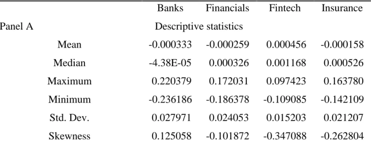
Table 2. decriptive statistics and correlation matrix for full sample period

Banks Financials Fintech Insurance

Panel A Descriptive statistics

Mean -0.000333 -0.000259 0.000456 -0.000158 Median -4.38E-05 0.000326 0.001168 0.000526 Maximum 0.220379 0.172031 0.097423 0.163780 Minimum -0.236186 -0.186378 -0.109085 -0.142109 Std. Dev. 0.027971 0.024053 0.015203 0.021207 Skewness 0.125058 -0.101872 -0.347088 -0.262804

Kurtosis 17.80579 15.40292 9.952486 13.53184 Jarque-Bera 20931.52* 14688.54* 4660.175* 10614.57*

Panel B Correlation matrix

Banks 1

Financials 0.950246* 1

Fintech 0.749575* 0.853332* 1

Insurance 0.83443* 0.925606* 0.850966* 1

Notes: Panel A shows the descriptive statistics for the daily log return of S&P FINANCIAL SEL. SEC. index, S&P500 BANKS index, S&P500 INSURANCE index, and KBW Nasdaq

Financial Technology Index (KFTX) from 3 January 2007 to 9 February 2016; Panel B is the coefficient of correlation. The data consist of 2292 daily observations.

*Indicates the rejection of the null hypotheses at the 5% level.

All the data are daily closing price and cover the period from 3 January 2007 to 9 February 2016, and the daily price are tranformed into log return in order to make the data free from autocorrelaion, which is also often adopted by previous researchers. The Banks in the results table of this article represent the logarithmic return of the S&P500 BANKS index, Financials poxy for the log return of the S&P FINANCIAL SEL. SEC. Index, Fintech represent the KBW Nasdaq Financial Technology Index (KFTX), and Insurance proxy for the S&P500 INSURANCE index.

Panel A provides the basic descriptive statistics for log return of four variables, the average return is -0.033% for Financials with volatility (the standard deviation, which is the proxy for volatility) of 0.028, -0.026% for Banks with volatility of 0.024, 0.046% for KFTX with volatility of 0.015, and -0.016% for Insurance with volatility of 0.021, both indices of financial sector bears higher risk with low average return, while KFTX has lower risk with higher average return, which means that the KFTX is a more worthy investment. The theoretical kurtosis value for a Gausian probability distributions is 3 to indicate the normality distribution of the series, however, the kurtosis value of all variables under detected are higher than 3, which implying that none of these returns follow the nomality patterns, skewness is a measure for the lack of symmetry, all the

series are negatively skewed except for banks, which reveals that there is an leptokurtic distribution and asymmetric tails for each 𝑅𝑅_𝑡𝑡 , Jarque-Bera test can test whether the sample has proper skewness and kurtosis value that matching the normal distribution (Ramona & Mihail, 2014), the results are reject the null hypothesis of normal distribution, further explains that the data do no normallly distributed.

Panel B presented the correlation matrix between these variables, the correlation

coefficient between Fintech and the Banks, Financials, and Insurance are 0.75, 0.85, and 0.85 respectively, this indicate that the indices of these sectors are closely linked,

suggesting that there may exist the interactive behavior between fintech sector and traditional financial sectors, in order to prove the existance of this relationsip, the Granger Causality VAR test are adopted and further use the Yoda yamamoto Granger causality test to verify the results.

The prerequisite of Granger -causality test is that the series needs to be stationary (Dickey & Fuller, 1979), thus, the Augmented Dickey-Fuller(ADF) test is adopted to detect the unit root of variables, table 3 shows that the t-statistics of these four series are significant at 95% confidence interval, additionally, the probability value is also below 5%, we conclude that all the variables are stationay at 5% sinificant level, this resut is not surprising because the log return as mentioned by (Ajaya & Swagatika, 2018) and (Yinqiao, Renée, & Laurens, 2017) in their articles will make the financial series become stationary.

Table 3 Augmented Dickey–Fuller (ADF) Test 2007-2016

Index t-statistic p-value

Banks -53.68043* 0.0001

Financial -54.58079* 0.0001

Fintech -51.68511* 0.0001

Insurance -54.78237* 0.0001

Notes: the unit root test is applied to the log return of each indices. *Denotes statistical significance at the 5% level.

6.1.1 Autocorrelation and inverse roots

Before applying the causality test under VAR framework between those two sectors, the optimum lag length is choosing based on the information criteria (lowest Akaike information criterion). Once the optimum lag structure has been chosen, as (Bouri, Jain, Biswal, & Roubaud, 2017) and (Anupam, 2018) suggested, the autocorrelation test is carried out among the residuals to check whether the selected model is fitted under study. But since the existence of the serial correlation at lag 6 for Financials and Fintech during the full sample period, thus we add four extra lags to the optimum lags choosing by information criteria to eliminate the autocorrelation of the residuals. The results of the optimum lag length for each indices is show in table 5 together with the cointegration results. Finally, the AR roots Graph has plotted for each pairwise(Appendix), if all the roots for each index pair are within the unit circle. the VAR model is stable(stationary), see Lütkepohl (1991). The results of inverse roots indicate that the model under study is stable, thus, further studies is carried out in the next part. which is a good result and indicate that the selected model is fitted to each 𝑅𝑅_𝑡𝑡, the results of autocorrelation test and optimum lag are presented in the appendix for reference.

6.1.2 Granger causality test for full sample period

Table 4 Granger Causality Test 2007-2016

Pairwise index P-value (1) P-value (2) Banks & Fintech 0.0051 0.0024 Financials & Fintech 0.0097 0.0331

Insurance & Fintech 0.2612 0.9683

Notes: P-value (1) denotes the Granger causality test for the first market Granger-causes the second market; P-value (2) denotes the Granger causality test for the second market Granger-causes the first market. Null hypothesis: no causality from financial sectors to fintech for value (1); no causality from fintech to financial sectors for

For the full sample period from 2007 to 2016, p-value (1) and p-value (2) for both index pairwise of Fintech & Banks, and for Fintech & Financials are below 5% significant level, meaning that the null hypothesis of one index do not granger cause another index is rejected, thus, the bi-directional granger causality is detected between S&P500 BANKS

index and KFTX, and between S&P FINANCIAL SEL. SEC. index and KFTX, but since

both the p-value (1) and p-value (2) for Insurance & Fintech are much higher than 5%, we can not reject the non-causality hypothesis, S&P500 INSURANCE index and KFTX do not have causal relationship during the full sample period.

Such results are expected, firstly, the bank’s industry involves the conversion of material goods, people, and information and is considered to be a pioneer in the use (rather than creation) of information technology (Freeman, 1991) (Utterback, 1994) (Voss, 1994). Secondly, the fintech sector has brought technological innovation to the traditional financial sector and injected new vitality, while these innovations are changing the traditional player’s business landscape, just as (Jarunee, 2017) mentioned that in terms of banking landscape, fintech-based business innovation from ATMs, online banking, international electronic funds transfer, and electronic data exchange (EDI) to mobile banking, bitcoin wallets, blockchain banks, and crowdfunding has greatly improved the financial innovation system, but (Vives, 2017) argue that although in the fields of lending, asset management, portfolio advice and payment systems, the fintech sector is exerting an impact on the banking and capital markets, but even in the largest fintech market in China, the size of the financial technology industry is not enough to match the financial industry of the entire country, and considering that our full sample contains data from financial crisis period (which cased the index price to fluctuate greatly, especialy the financial industry indices, and the market instably guring the stress periods), we need to detect sub-samples of different periods.

6.1.3 Toda Yamamoto Granger Causality Test

The Toda Yamamoto (TY) version of Granger Causality test under VAR freamwork was developed by (Toda & Yamamoto, 1995). In practice, we did not know the true data-generating process (DGP), or we cannot sure that if the series under study have I(0), I(1), CI, or no CI. Jain & Ghosh (2013) mentioned that the TY-Granger Causality test mitigate the potential bias from unit root test and cointegration test, (Clarke & Mirza, 2006) also point that the TY-Granger Causality test has advantage over general VAR modeling since

the process such as first differences and pre-whitening of the series will leads to the sacrifices of long-run information, it aslo produces a greater probability of type 2 error (the power of the model will decrease, often leading us do not reject a false null hypothesis). In order to verify that the traditional Granger Causality test achieved the proper results, we further applied another robust method to validate the results,

Table 5: Johansen's cointegration Test

2007-2016

Fintech Fintech Fintech

Optimum lag 6 6 2

Banks 745.77 (437.32)

Financial 394.61 (228.85)

Insurance 812.15 (427.66)

Notes: The Johansen's Trace Test and Max. Eigenvalue Test are used to test multivariate cointegration with critical value of 95%; the number presented above are represent as:

t-statistic of Trace Test (t-t-statistic of Max. Eigenvalue Test)

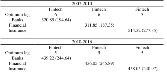
The pervious ADF test implying that all the 𝑅𝑅_𝑡𝑡 of each indices are stationary at level, or say, all the 𝑅𝑅_𝑡𝑡 have been integrated to I(0), therefore, Johansen cointegration approach is adopted to invistegate the long-run relationship among each 𝑅𝑅_𝑡𝑡 pairwise, the appropriate optimum lag structure is selected based on the Akaike or Schwarz Information criterion, as table 5 presented, t-statistic of both Trace Test and Max. Eigenvalue Test for indices are insignificant at 95% confidence interval, which reject the null hypothesis of non-conitegration beween two series, thus, a long-run association is existing among each indices pair under study (Rizwan Raheem, Jolita, Dalia, & Majid, 2017).

TY Granger Causality test control for potential unit roots by adding one extra lag above the optimum lag structure, as show in the table 6, we can see that both Banks and Fintech’s p-value (1) and p-value (2) are less than 5%, and the null hypothesis that there is no causality between the indices is rejected at a significant level of 5%, which indicate that there is a causal relationship between the Banks and Fintech, and these two sector indices have a linkage effect. While the two probability values between Insurance and Fintech are still greater than 5%, there is no causal relationship between the two. The result obtained by TY Granger Causality test are consistent with the results of the traditional Granger Causality VAR model, this is also proving that the relationship among these indices in the period 2007 to 2016 is rubost.

From the above empirical results, there is indeed an interplay between the financial sector index and the Fintech sector index from year 2007 to year 2016, with the exception of the insurance sector, this may due to the fact that the insurtech has developed rapidly only in recent years, and the industry scale is insignificant compared to the traditional insurance sector, and it is not enough to have an impact on the traditional incumbents (Bernardo, 2017).

Table 6 Toda Yamamoto Granger Causality Test 2007-2016

Pairwise index P-value (1) P-value (2)

Banks & Fintech 0.0047 0.0024

Financials & Fintech 0.0132 0.0369

Insurance & Fintech 0.2517 0.9845

Notes: P-value (1) denotes the Granger causality test for the first market Granger-causes the second market; P-value (2) denotes the Granger causality test for the second market Granger-causes the first market. Null hypothesis: no causality from financial sectors to fintech for P-value (1); no

6.2 Sub-period analysis

Since our sample includes the data during financial crisis, and such data will lead to different empirical results, we further use sub-sample analysis to study weather the relationship among the indices will changes under different maket conditions. Many previous researchers have also adopted the sub-period analysis to study the changes in the series relationship at differne times (in the critical period of the stress period such as financial crisis ). Batten, Kinateder, Szilagyi, & Wagne (2017) states that the subsample approch will faciliitate us to assess weather the causal relationship is evolves over time; Batten, Kinateder, Szilagyi, & Wagne (2017) also indicate that the dependency structure among the variables would have been significantly affected since the large upward moves are seen in the series during the stress period. It is therefore necesary and important to study if the relation between the fintech sector and traditional financial sector evolves over time.

One of our limitation here is that we can not investigate the charateristics of the relationship among thses series for the pre-crisis period since the fintech is a young field and we cannot find available data for the KFTX index before 2007. Thus, our data is divided into the financial crisis period (2007-2010) and the post-crisis period (2011-2016), the selection basis of our sample interval is the same as that of Polanco-Martínez, Fernández-Macho, Neumann, & Faria (2018), who studied the relationship between PIIGS and S&P Europe 350 index. They analysed two characteristic periods, one was the pre-crisis period (2004-2007), which was characterized by small index volatility and market growth; the second is the period of financial crisis (2008-2011), which is characterized by large market index volatility, the results of their study show that the causality between the two periods is inconsistent, revealing that the correlation between PIIGS and S&P Europe 350 index varies with time. Moreover, the time-scale (frequency) of the data used will also affect the results.

However, we cannot curenly infer whether the relationship between the indices we studied will also change over time, the steps of following empirical analysis are the same as those of the full sample period, but it is conducted srparately for the two sub-sample periods and the test results will be compared.

Table 7: Descriptive statistics and correlation matrix during the crisis period

Banks Financials Fintech Insurance

Panel A Descriptive statistics

Mean -0.001003 -0.000832 0.000265 -0.000737 Median -1.47E-03 -0.000595 0.001020 0.000251 Maximum 0.220379 0.172031 0.097423 0.163780 Minimum -0.236186 -0.186378 -0.109085 -0.142109 Std. Dev. 0.038872 0.033050 0.019147 0.028856 Skewness 0.179915 -0.011271 -0.243828 -0.167204 Kurtosis 10.68923 9.516311 7.828453 8.615240 Jarque-Bera 2486.187* 1781.669* 988.1929* 1327.677*

Panel B Correlation matrix

Banks 1

Financials 0.950439* 1

Fintech 0.745927* 0.858508* 1

Insurance 0.82474* 0.919667* 0.854786* 1

Notes: Panel A shows the descriptive statistics for the daily log return of S&P FINANCIAL SEL. SEC. index, S&P500 BANKS index, S&P500 INSURANCE index, and KBW Nasdaq

Financial Technology Index (KFTX) from 3 January 2007 to 31 December 2010; Panel B is the coefficient of correlation. The data consist of 1008 daily observations.

*Indicates the rejection of the null hypotheses at the 5% level.

Table 8：Descriptive statistics and correlation matrix during post-crisis period

Banks Financials Fintech Insurance

Panel A Descriptive statistics

Median 0.000507 0.000629 0.001319 0.000717 Maximum 0.067587 0.078875 0.054521 0.077847 Minimum -0.097651 -0.105186 -0.08614 -0.084873 Std. Dev. 0.014527 0.013245 0.011185 0.012220 Skewness -0.439091 -0.419926 -0.518233 -0.214146 Kurtosis 7.866746 9.852975 7.921945 8.796251 Jarque-Bera 1307.400* 2548.285* 1352.486* 1805.821*

Panel B Correlation matrix

Banks 1

Financials 0.951187* 1

Fintech 0.821413* 0.882933* 1

Insurance 0.887286* 0.954024* 0.872502* 1

Notes: Panel A shows the descriptive statistics for the daily log return of S&P FINANCIAL SEL. SEC. index, S&P500 BANKS index, S&P500 INSURANCE index, and KBW Nasdaq

Financial Technology Index (KFTX) from 3 January 2011 to 9 February 2016; Panel B is the coefficient of correlation. The data consist of 1284 daily observations.

*Indicates the rejection of the null hypotheses at the 5% level.

The basic descriptive statistics and correlation matrix for the two sub-periods are shown in the above table, table 7 shows the statistical results during the financial crisis period, it can be seen that the average logarithmic returns of S&P FINANCIAL SEL. SEC. index, S&P500 BANKS index, and S&P500 INSURANCE index during this period are all negative and accompanied by higher volatility (risk), however, the KFTX has a higher and positive return, while also bearing a smaller risk. These results are similar to the results of the full-sample period and both show that the KFTX is more worth investing.

Table 8 shows the statstical characterstics of each 𝑅𝑅_𝑡𝑡 after the financial crisis. It can be seen form Panel A that the average return of each indices are positive from 2011 to 2016,

the yield of KFTX is still higher than the other three indices, yet the gap between those indices is not as large as it is during the financial crisis. However, the volatility of each index after the financial crisis only accounted for one-half or one-third before the financial crisis. Results of kurtosis and skewbess also reveals that the data are non-normality distributed during two different periods.

Panel B of upper two tables provide the correlation coefficient between fintech and banks, fintech and insurance, as well as fintech and financial services sector. All coefficients are significant at 5% significant level for both crisis period and post-crisis period. The correlation between those sector pairwise are more closer during post-crisis period than crisis period.

6.2.1 Granger Causality Test for sub-sample periods

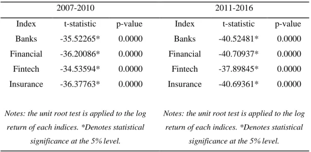
Augmented Dickey–Fuller (ADF) test for each period are applied to all the series before further test, table 9 exhibit the results of unit root test for sub-sample. We can see that all the t-statistics for log return of each indices are significant, and p-value is smaller than 5%, which indicate that all the series are stationary at 5% significant level for both crisis and post-crisis period.

Table 9: Augmented Dickey–Fuller (ADF) Test

2007-2010 2011-2016

Index t-statistic p-value Index t-statistic p-value

Banks -35.52265* 0.0000 Banks -40.52481* 0.0000

Financial -36.20086* 0.0000 Financial -40.70937* 0.0000 Fintech -34.53594* 0.0000 Fintech -37.89845* 0.0000 Insurance -36.37763* 0.0000 Insurance -40.69361* 0.0000

Notes: the unit root test is applied to the log return of each indices. *Denotes statistical

significance at the 5% level.

Notes: the unit root test is applied to the log

return of each indices. *Denotes statistical significance at the 5% level.