Evaluating Bluetooth Radio for Physiological Monitoring

(1)

Mälardalen University

School of Innovation, Design, and Engineering

Västerås, Sweden

Thesis for the Degree of Bachelor of Science in Engineering -

Computer Network Engineering 180 credits

Evaluating Bluetooth Radio for Physiological Monitoring

Aymen Al-Ramadan

aan13011@student.mdh.se

Examiner: Mats Björkman

Mälardalen University, Västerås, Sweden Supervisor: Hossein Fotouhi

(2)

Abstract

Globally, population numbers are growing, and the lifespan of the elderly is increasing. Therefore, this phenomenon requires that society commit more money, facilities, and staff for health care. The Internet of Things (IoT) can be employed to cover the financial shortfall in healthcare resources by using sensors for remote health monitoring such as the Shimmer device. The Shimmer physiological sensor is a Bluetooth-enabled radio device designed and used for monitoring various human health conditions. Using a sufficient number of the Shimmer devices with proper sampling rate can affect the provision of health and related information in real-time. Moreover, this type of sensor can sometimes be attached to the human body, which can create an inference between the sensors and the human body. The high-noise environment may also impact the sensor. This thesis reviews and analyses several scenarios in which Shimmer devices can be used by medical practitioners to offer reliable physiological measurements, such as ECG and movement. This study found that the Shimmers device can provide reliable data by using a specific configuration when the maximum number of sensors participate in a piconet network.

(3)

Acknowledgement

There is a commonly used technical IT term called “slave”. The term refers to the device or node that is engaged in piconets topology. The topology is based on the master unit that controls up to seven nodes. We ask to be excused from using this term. Accordingly, whenever the reader sees the word “node” and it is related to piconet topology or a master unit, it should be assumed that it is referencing the term “slave unit”. Although, we did use the term once in Chapter 2, Background for the sake of clarity and to refresh the reader’s memory in the event they forgot having read this statement.

(4)

Abbreviations

ACL Asynchronous Connectionless

BLE Bluetooth 4.2 Low Energy

CDMA Code-Division Multiple-Access COTS Several commercial-off-the-shelf

CSMA/CA Carrier Sense Multiple Access with Collision Avoidance

ECG Electrocardiogram

EDA Electrodermal Activity EMG Electromyogram

FHSS Frequency-Hopping Spread-Spectrum GFSK Gaussian Binary Frequency Shift Keying GUI Graphical user interface

IoT The Internet of Things

L2CAP Logical Link Control and Adaptation Layer Protocol MDH Mälardalen University

Node Slave unit in a piconet network RMH Remote health monitoring RSSI Radio Signal Strength Indicator SSP Secure Simple Pairing

WLAN Wireless local area network WPANs Wireless Personal Area Networks

(5)

Table of Figures

Figure 1: WSNs topologies [5]. ... 3

Figure 2: The Bluetooth protocol stack [12]. ... 5

Figure 3: Channels & time slots in the Bluetooth medium [18]. ... 6

Figure 4: Non-overlapping among the channels. ... 7

Figure 5: Overlapping among the channels. ... 7

Figure 6: Example of a shimmer configuration ... 10

Figure 7: Position of the master unit and the Shimmer devices from different distances. ... 12

Figure 8: Screenshot of the captured wireless signals around the environment. ... 12

Figure 9: Wireless signals in Mälardalen university library. ... 14

Figure 10: 802.11b/g signal coexists with 802.15.2 signal. ... 15

Figure 11: The propagation of the wireless channels in the library ... 15

Figure 12: Comparison the RSSI values for seven experiments when the Shimmer devices are placed on the desk with sampling rate 512Hz from a 1m distance. ... 16

Figure 13: Comparison the RSSI values for seven experiments when the Shimmer devices are placed on the desk with a sampling rate 512Hz from a 1m distance. ... 16

Figure 14: Comparison the RSSI values for seven experiments when the Shimmer devices are placed on the desk with a sampling rate 512Hz from a 3m distance. ... 17

Figure 15: Comparison the PRR values for seven experiments when the Shimmer devices are placed on the desk with a sampling rate 512Hz from a 3m distance. ... 17

Figure 16: Comparison of the RSSI values for seven experiments when the Shimmer devices are placed on the desk with a sampling rate 512Hz from a 5m distance. ... 18

Figure 17: Comparison of the PRR values for seven experiments when the Shimmer devices are placed on the desk with a sampling rate 512Hz from a 5m distance. ... 18

Figure 18: RSSI Comparison without interference among different sampling rates of 256Hz, 512Hz and 1024Hz with the maximum number of sensors in the piconet network. ... 19

Figure 19: PRR Comparison without interference among different sampling rates of 256Hz, 512Hz and 1024Hz with the maximum number of sensors in the piconet network. ... 20

Figure 20: Comparison of RSSI values between 7 Shimmer devices on the desk and 7 Shimmer devices attached to the body with a sampling rate of 512Hz ... 20

Figure 21: Comparison of PRR values between 7 Shimmer devices on the desk and 7 Shimmer devices attached to the body with a sampling rate of 512Hz ... 21

(8)

Figure 23: PRR comparison among 7 Shimmer devices on the desk, 7 Shimmer devices

attached to the body from 5m, and 7 Shimmer devices attached to moving body ... 22

Figure 24:RSSI comparison between 7 Shimmer devices on the desk and without interference and 7 Shimmer devices on the desk in a high-noise environment with a sampling rate of 512Hz. ... 22

Figure 25:PRR comparison between 7 Shimmer devices on the desk and without interference and 7 Shimmer devices on the desk in a high-noise environment with a sampling rate of 512Hz. ... 23

Figure 26: Comparison of RSSI values among 1 Shimmer on the desk without interference, Wi-Fi router in the middle of Shimmer connection, and 1 Shimmer in a high-noise environment. Sampling rate 512Hz. ... 23

Figure 27: Comparison of RSSI values among 1 Shimmer on the desk without interference, Wi-Fi router in the middle of Shimmer connection, and 1 Shimmer in a high-noise environment. Sampling rate 512Hz. ... 24

Table of Formulas

Formula 1: Channels in Bluetooth ... 6

Formula 2: RSSI (log-normal shadowing path-loss) ... 7

Formula 3: The physics formula of the sampling rate. ... 8

(9)

Introduction

In general, young people are less likely to need to monitor their health status Frequently. People may of course watch their sports activities sometime for a useful purpose such as to see how many calories have been burned during the exercises. On the other hand, health care in developed countries has another reason for paying attention to remote health monitoring (RHM). In some situations, a patient needs to stay at the hospital for several days, just to get accurate results of his/her health status. That leads one to wonder what will happen when the number of patients needing such monitoring grows daily beyond the systems current limitations? It will cost society a lot of money to meet this growing need. However, if the money is not an issue, the resources and health care quality will suffer from the pressing need to accommodate the additional patients. Records contained in the report entitled, “World Population Ageing” published by the United Nations, show that people in this segment of the population over the age of 59 will increase by more than 55 percent between the years 2015 and 2030. Moreover, people with age 79 and older will be 430 million by the year 2050 that considers all world [1]. Therefore, remote health monitoring will be considered as a new era of smart health care. This new method will facilitate a physician’s ability to check and analyse a patient's condition online. If this method is used increasingly during the timeframe indicated societal health care needs might be better addressed on a greater scale through the use of multiple sensors networks. The coexistence of several sensors might create for example an interference or even impact the performance of the network. Therefore, one of focuses of this thesis is to study the impact of data sent from several physiological sensors. In achieving this goal, several Shimmer devices containing physiological sensors are utilised and tested by this thesis for the purpose of this study.

1.1 Problem Formulation

There are several commercial-off-the-shelf (COTS) physiological devices with a wireless connection that is available for purchase. However, there is a lack of comprehensive evaluation of such devices to show their ability in practical usage within a clinical environment. The study has defined the problem into the following sub-problems:

1. How many physiological sensors can operate reliably in a network? 2. What is the impact of the human body on measurements?

3. What is the impact of human movement on measurements?

4. What is the impact of interference from other devices operating on the same frequency domain in terms of the performance of a network?

1.2 Ethics

By law, the security and confidentiality of patient records, data, and related information should be guaranteed by health care providers. All tests and studies presented in this thesis were carried

(10)

Background

This chapter describes briefly the protocols and technologies that are used in this thesis. It also introduces an overview of Consensys software for Shimmer devices configuration. Furthermore, it explains concisely the python script that collects data from remote physiological sensors.

2.1 Overview of Wireless Sensors Networks (WSNs)

Wireless Sensors Networks (WSNs) are considered as a key of the Internet of Things (IoT). WSNs are widely used in various application areas such as environmental and structural monitoring systems, industrial automation, healthcare systems, traffic management and logistics, and public safety. An efficient IoT-enabled healthcare system aims to provide a remote health monitoring capability of a patient’s health status in real-time. In addition, it offers the prevention of critical patient conditions, improvement of the quality of life of the elderly through use of the smart environment, medical and drugs' database administration, and well-being services. Use of smart IoT sensors for improving the delivery of healthcare enables the accurate measuring, monitoring and analysing a variety of health status indicators together with environmental parameters [2]. A wireless sensor network refers to independent wireless sensors that have to monitor and collect data, then transferring the information to a database or a cloud server. It is very likely that for the sensors in WSNs to communicate efficiently with each other largely depends on a proper network configuration. Eventually, all collected information is directed wirelessly to a central node, which is called the Master Unit. In the WSNs, sensors can be divided into two types: the high-power sensor and low-power sensor. The high-power sensor refers to the sensor that consumes high energy from the battery or energy source, compared to the low-power sensor. Therefore, each type of sensor has to have specific protocols that can make it capable of communicating properly. A sensor typically consists of a power source (usually an AA battery), a microcontroller (CPU collects the data to flash memory), a transducer (translates the environmental variables to electrical signals), and, a transceiver (transmits the radio signal for the communication purpose) [3].

2.1.1 Topologies of WSNs

Broadly speaking, in the WSNs the structure may be designed by one of three forms of network topology: (i) star, (ii) mesh, and (iii) tree topology.

A. Star Topology (piconets)

In this form of the network, the nodes (slaves) do not communicate with each other. Instead, they communicate directly with the master unit. Consequently, the master unit is considered as a getaway that controls data sent to every single sensor. Also, the data transmission in the network is self-configured and does not need to be routed. This topology can allow the network to expand flexibly by adding more nodes without changing any network configuration. Nodes should be located within the area of the radio frequency signal transmitted by the master unit. However, if any node goes offline, this will not impact the network, excluding the master unit.

(11)

Figure 1 illustrates the design of the star topology, moreover this topology is called piconets in Bluetooth technology.

B. Tree Topology

In the tree topology, the design of the network is based on the concept of parent and children. The master unit is shown on top of the tree and is considered the root. The root is connected to several nodes, which makes the node a child of the root. Every child in the tree can be a “parent” by also having a child. These children can go on to create a level of communication between parents and their children. Consequently, the traffic that is sent by a child should go through its parent/parents to reach the root (master unit). If one of the parents fails, the children of that parent will not be able to communicate with the root (master unit) or with nodes that are connected to their parent. Figure 1 illustrates the design of tree topology.

C. Mesh Topology

In this type of network, every node can connect with other nodes in order to provide a significant coverage area for a single wireless network. Usually, multiple gateways are used in a wireless mesh network for the purpose of providing redundant connectivity to the wireless network. The data travels from one node to other nodes within the same wireless coverage. This network topology has many advantages, but the best primary advantage is its prevention of a single point of failure. Figure 1 illustrates the design of mesh topology [4].

(12)

2.2 Wireless Protocol

In some situations, such as a swimmer wanting to monitor his/her heart rate during the exercises, the energy source of the sensor must be mobile in order to affect its usability. Moreover, the energy source should provide enough energy during the entire time of use so that the swimmer can rely on its use. Therefore, wireless systems need protocols that consume low energy in order to be suitable for wireless devices. These devices usually have very weak processors that utilize low energy levels. Furthermore, such processors do not require a long-range radio frequency because they are usually placed close enough to the target and (master unit). There are several protocols that are designed for such requirements, e.g., IEEE 802.15.1 and IEEE 802.15.4.

2.2.1 Bluetooth (IEEE 802.15.1)

Before going through the technical information about IEEE 802.15.1, it is good to know what the name references. This part of the protocol’s name “IEEE 802.15” refers to a working group that develops the WPANs standard (Wireless Personal Area Networks) and the last part that ends with a number refers to the version of the standard, which is known by name Bluetooth [6]. The specification for version 1.0 of IEEE 802.15.1 standard was released in 1999 [7]. Bluetooth is a wireless data communication protocol that has a characteristic of short-range radio frequency. It is an open standard protocol that is established to replace the wire-connection for devices using peer-to-peer connectivity. Bluetooth utilises global unlicensed radio frequency signal 2.4 GHz up to 79 channels with 1 MHz for each channel space. This range of frequencies can be less than that in some countries. The radio frequency in Bluetooth can deliver a signal to 10 m without any obstructing object in the “line-of-sight”. In the ideal situation, the modulation Gaussian Binary Frequency Shift Keying (GFSK) allows the data to be transmitted in the Bluetooth medium by 1 Mbit/s [8].

The network topology for Bluetooth can contain eight piconets, one as a single master unit and the others as the active nodes. The Bluetooth topology follows the same principle of Star topology mentioned before, but here it is called piconets [9]. In order to avoid collision and interference in the Bluetooth medium, the data transmission method used is based on a combination of two techniques (FH-CDMA), Frequency-Hopping Spread-Spectrum (FHSS) and Code-Division Multiple-Access (CDMA). FHSS is a modulation technique that provides fast jumping 1600 hops/sec among the 79 frequencies. It transfers multiple data by using the whole range of frequencies. Moreover, it utilises a small space of a single frequency to carry a part of the data, instead of using them all. The cooperation between CDMA technique and the FHSS allows the other Bluetooth devices in the piconets to transmit data at the same carrier frequency. That makes CDMA responsible for the division of multiple access. Moreover, the master unit controls the communication through the hopping sequence and access channel. Thus, every piconet in the network should synchronise its clock with the master to get the right frequency hopping and then to be allowed to transmit data [8, 10, 11].

Understanding the Bluetooth protocol stack will facilitate a network administrator’s ability to evaluate the performance of piconets. The Bluetooth protocol stack describes the architecture

(13)

of Bluetooth protocol layers. Thus, the network administrator can understand how the frame transmits in the Bluetooth medium.

The stack consists of three logical groups as it is shown in Figure 2:

The transport protocol group. This group is responsible for radio communication

linkage and interoperability with upper layers. It contains:

i. Radio layer: This layer operates radio frequency 2.4 GHz ISM.

ii. Baseband layer: This layer manages how the data will be sent over the

Bluetooth medium. Therefore, it controls two types of links; the first one is a link that can send a high priority data once in a while such as voice. This type of link called Synchronous Connection-oriented (SCO), the second one is Asynchronous Connectionless (ACL) for sending a standard data that has the ability to re-send.

iii. Link Manager layer: This layer controls the air-interface link between devices.

The term air-interface includes many things such as the negotiation of power activity, authentication between devices, trust between devices, and encryption.

iv. L2CAP: This layer is responsible for fragmentation and maintaining data.

Furthermore, it receives a data from upper layers and converts it to a form that can send by the Bluetooth medium. Likewise, if it receives data from lower layers, the data will be converted to be a suitable format for the application layer.

The middleware protocol group manages the transmitting process of applications

through the Bluetooth links.

The Application group is responsible for managing the applications [12].

(14)

2.2.2

IEEE 802.15.2 + Enhanced Data Rate

Bluetooth version 2.0 is based on Bluetooth version 1.0 and is still compatible with it. On version 2.0 the data rate has been enhanced to support a maximum speed of 3 Mbps while version 1.0 has a maximum speed of up to 1 Mbps as mentioned previously [13]. Moreover, the security of Bluetooth version 2.1 has improved with a new function that is called Secure Simple Pairing (SSP). With this functionality, the communication between Bluetooth devices will not be allowed until the device passes the same pin code to confirm the security condition and make the traffic encrypted [14, 15]. Since Bluetooth uses an unlicensed frequency, it might create some interference with other wireless networks that use the same range of frequencies. This version of Bluetooth also includes the coexistence mechanism to avoid the interference among unlicensed signals or at least to mitigate it [16]. Although, the data still spread over the 79 channels at 1600 hops/second with the nominal time slots 625 us. Figure 3 emulates data transfer in sequence via the Bluetooth spaces. Formula 1 below represents the channels, where k refers to the number of the current channel:

f = 2402 + k MHz, k = 0, ...., 78 [17]

e.g. When k has a value 2MHz, the frequency becomes; f = 2402 + 2 = 2404 MHz

Figure 3: Channels & time slots in the Bluetooth medium [18]. 2.2.3 Wi-Fi (IEEE 802.11b/g)

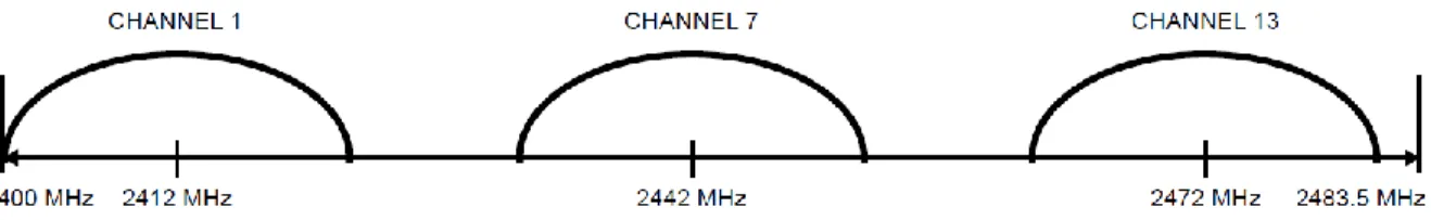
IEEE 802.11b/g is a standard protocol for a wireless local area network (WLAN). The 802.11b is the new standard after the first standard IEEE 802.11, which comes with an enhanced data rate and coexistence with other unlicensed frequencies. On the other hand, IEEE 802.11g is the amended version to 802.11b, and it is backward compatible with 802.11b. The protocol is used widely and is directed primarily for home/office use. It supplies network connection among devices through a radio signal. The signal is considered a long-range radio frequency, which can reach approximately a 100-meter distance. The transmitter in 802.11b/g generates an unlicensed radio frequency 2.4 GHz to 2.483 GHz with 13 channel spaces in most of European [19]. Each channel space comes with bandwidth 22 MHz to avoid the overlapping among

(15)

channels. In the ideal situation, IEEE 802.11b offers 11 Mbps speed by employing the complementary code keying (CCK) with DQPSK modulation, while IEEE 802.11g provides up to 54 Mbps by utilising coding OFDM and 64QAM modulation. The traffic in 802.11 environment controllers by the protocol Carrier Sense Multiple Access with Collision Avoidance (CSMA/CA) [20]. In Figure 4, channels are configured with non-overlapping. Likewise, the frequencies interfere with each other as shown in Figure 5 [21].

2.3 Technical Terms

This section is devoted to explaining the technical terms that are used in this study.

2.3.1 Radio Signal Strength Indicator (RSSI)

RSSI refers to a value that estimates the wireless signal strength between two nodes. The estimation is not based on development hardware. Instead, it is based on a mathematical algorithm [22]. The algorithm which is called log-normal shadowing path-loss describes the relation between the RSSI level and the distance. Furthermore, in a more complex algorithm, the target's transmitter power may be considered as one of the factors that influence the RSSI level. Consequently, the RSSI can also indicate the quality of the signal [23].

RSSI = 10nlog(d), where n is the propagation constant and d is corresponding to distance [24].

Usually, the value starts from RSSI = 0dBm to indicate the best situation of a signal that can be achieved. After that, the value goes down in minus digits pointing out the deterioration in the signal. Thus, the bad metric of the RSSI can lead to errors in data transmission [16, 25]. In

Formula 2: RSSI (log-normal shadowing path-loss) Figure 5: Overlapping among the channels. Figure 4: Non-overlapping among the channels.

(16)

2.3.2 Sampling Rate

The term sampling rate is utilised mostly in audio environment or applications. The process of sample rate specifies how many samples of data that should be collected from an environment in a period (usually in one second) [27]. Sampling is performed by using a particular processor for converting the data from analogue to digital form. The same method is used by a physiological sensor that monitors the status of health such as an electrocardiogram (ECG) [28]. Reporting the status of health is considered more accurate when the physiological sensor is able to gather larger amounts of data and information per second.

𝑓𝑠 = 1

𝑡 (the metric by hertz and t refers to time) [29]

For example, a sensor that has been configured with a sampling rate of 10 Hz should collect ten packets per second. On the other hand, the sensor that has been set at 512 Hz, is supposed to collect much more measurements [30].

2.3.3 Packet Reception Ratio (PRR)

The term PRR as used in this thesis is related to the term sampling rate and RSSI. The result of the mathematical formula of PRR shows the ratio of how many packets have been delivered to a network device. The formula calculates the relation between the number of packets that should be delivered to the network device and the number of packets that are received [31, 32]. Formula 3 below is used to calculate the sampling rate ratio.

𝑃𝑎𝑐𝑘𝑒𝑡𝑠𝑟𝑒𝑣𝑒𝑖𝑣𝑒𝑑

𝑃𝑎𝑐𝑘𝑒𝑡𝑠𝑔𝑒𝑛𝑒𝑟𝑎𝑡𝑒𝑑 × 100 = PRR% [32]

In other words, PRR represents the quality of service (QoS), which can be affected by the RSSI or the sampling rate [33].

2.3.4 RFCOMM

One of the primary purposes of developing a Bluetooth protocol is to replace the RS-232 cable. The RS-RS-232 cable was a conventional method of transferring data via serial port between two devices such as a personal computer and printer or modem. In the Bluetooth stacks, there is a transport protocol called RFCOMM that emulates the serial port by creating a connection channel over the lower layer (L2CAP) protocol. It has a mechanism to provide a complete communication between two Bluetooth devices (up to 60 connections) by controlling the data flow. The channel that is created by L2CAP for RFCOMM connection is responsible for acknowledging conversion of data between the two Bluetooth devices. Therefore, when the connection fails, the RFCOMM stops

Formula 3: The physics formula of the sampling rate.

(17)

sending data. This procedure ensures the reliability of all packets received in order, without the need of the resending method or the duplicated packets issue [34].

2.3.5 Blueman Software

Blueman is a free application that is compatible with the Raspbian distribution of Linux. It comes with graphical user interface application (GUI) to facilitate the management of the Bluetooth connection, instead of using the command line. Blueman can manage the paring process among piconets and make the communication flows through the RFCOMM protocol between the master unit and its nodes [35].

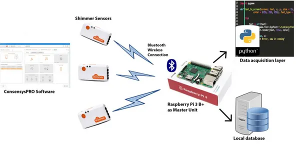
2.4 System Components

The following chapter describes the components of the network in this thesis as it is shown in Figure 3.

2.4.1 Physiological Wireless

As previously stated, the Shimmer is a wireless physiological sensor used to monitor the status of various health elements. These sensors are used to measure various physiological parameters such as Electrocardiogram (ECG), Electromyogram (EMG), Electrodermal Activity (EDA), heart rate and Galvanic Skin Response [36, 37]. The use of the Shimmer depends on the device’s type and characteristics. By default, there are two options for the user to store physiological data: either locally or on the master unit by streaming the data through Bluetooth. The Shimmer3 device comes with a microcontroller that provides Bluetooth 2.1 + EDR [38].

(18)

2.4.2 Consensys-Basic

Consensys is a free licence software that is used to configure Shimmer devices. It is compatible with Microsoft operating system. There are several features that are provided by Consensys-Basic including such things as, changing the sampling rate, managing the type of data collection and streaming the data in real time [39]. An example of the configuration method is shown in Figure 6.

2.4.3 Data Acquisition Layer (Python script)

The information that is streamed by Shimmer3 devices is sent to a script that is written in Python language. The script is an open source code. The part of the python script that is responsible for creating communication with the Shimmer3 devices was developed by the Shimmers Research Group [40]. The second part of the script allows for storage of data locally on the master unit. This segment of the script was developed by the group working on this thesis. Python is a high-level computer language with an open source license. It comes with some standard libraries that can be executed on many different operating systems such as Windows, macOS and most distributions of Linux [41].

2.4.4 Master Unit and Database (Raspberry Pi B+)

The aim of the master unit is to create a piconets topology with Shimmer3 devices. It stores local data sent by physiological sensors. The Raspberry Pi B+ is the latest model of the Raspberry Pi series (released 2018). The optimal operating system for use in the Raspberry Pi is Raspbian, which is based on Debian/Linux operating system. The free operating system “Raspbian stretch with desktop” comes with a graphical user interface (GUI) and a pre-installed version of the Python language [42]. The most remarkable hardware update related to the Raspberry Pi B+ is its chipset for wireless connectivity that supports Bluetooth 4.2 Low Energy (BLE) [43]. The BLE is also backwards compatible with Bluetooth 2.1 + EDR [44].

(19)

Methodology

This study began with a literature review of the health monitoring testbeds and Shimmer physiological sensors. MDH has some Shimmer devices and software to collect and measurements. It is essential to understand the tools and software that have been developed so far before starting new experiments. The tools reviewed consisted of the master unit, python, data collection through python script, and a Shimmer device as a node unit. It is mandatory to get RSSI measurements at the gateway side of the study in order to analyse radio characteristics for different environmental conditions. In order to solve the problems, this thesis encompasses the following experimental studies of:

1. The impact of adding nodes by varying number of Shimmer devices from one to seven (maximum possible devices in a Bluetooth-enabled network).

2. The impact of the data rate on the overall network performance by varying the sampling rate.

3. The impact of the human body by comparing the scenarios where the Shimmer devices are placed on a desk, and other Shimmer devices are attached to the human body.

4. The impact of node mobility and speed when a person walks at different speeds. 5. The impact of interference by adding a Wi-Fi router that operates ISM band (2.4

GHz) in the middle of the experimental area.

3.1 The Calculation Methods for the RSSI and PRR

The Shimmer devices ran over a period of around 10 minutes. Subsequently, the study chose to use 2 minutes of that period to evaluate the data received during the period. The results for each single Shimmer device were taken by computing the average value of RSSI, and the total number of packets delivered for PRR. Thereafter, if one of the experiments encompassed more than a single Shimmer device, the average of the RSSI for all Shimmer devices was considered in order to indicate to the approximate value that should result given a repeat of the same scenario.

(20)

Experiment Setup

This chapter describes the experimental environment setup and configurations. Most of the experiments were accomplished at home, except a single experiment at MDH library. The unwanted, troublesome sources of 2.4 GHz radio frequencies were considered in conducting the study. We utilised spectrum analyser software to discover surrounding Wi-Fi signals that were potentially creating interference for our experiment. Consequently, all experiments were run without any interference from other sources. Figure 7 shows the positions of the master unit and the Shimmer devices at different distances.

Figure 8 below shows the wireless signals that were captured during the experiments. The router with the name “Light” in the list of SSID is powered off during the experiments. The Figure displays that there were very week signals operating in 2.4 GHz surrounding the home, meaning that there were very low interference.

Zooming on the captured signals

Figure 7: Position of the master unit and the Shimmer devices from different distances.

(21)

4.1 Impact of Number of Nodes

The aim of this experiment was to study the first problem of the thesis on “The impact of some

nodes by varying number of Shimmer devices from one to seven”. We configured the Shimmer

devices by using Consensys-Basic. The configuration included: using the sampling rate of 512Hz which means sending 512 packets per second and making Bluetooth frame format 18 bytes total, which encompassed the data of low-noise accelerometer, wide-range accelerometer, and battery voltage. We couldn’t use just an ECG sensor, because not all Shimmer devices are created for the same purpose. Therefore, this frame size format emulates the most common scenario for using Shimmer devices such as ECG, EMG or respiration. As for the master unit, we used Blueman software for pairing with other Shimmer devices and for creating RFCOMM for every single connection. Thereafter, we started with a single Shimmer that was sending data to the master unit from a distance of one meter. Regarding the distance, the Shimmer was stationary, placed on a small plastic table. The last step was the execution of the python script for 5-10 minutes period to collect the data. The master unit stored two files for every single Shimmer; one for RSSI value and the other one for the data. The script queried new RSSI value every two seconds, whereas the file of data recorded every single packet that was received with a timestamp and number. After the scenario with a 1m distance, the same procedure was repeated for the scenarios with a 3m distance and 5m. Afterwards, we increased the number of Shimmer devices to seven. We observed at the beginning of executing the python script, the storing process could not collect data from all Shimmer devices simultaneously. There was always about a 5 to 20-second delay before all Shimmer devices would start to send the data. Accordingly, we chose and analysed data from the database for the 2 minutes period after comparing the timestamps among the database. We followed this process in order to be assured that all Shimmer devices sent the data to the master unit at the same time.

4.2 Impact of Sampling Rates

This experiment included a review of a second problem, “The impact of data rate on the overall

network performance by varying the sampling rate”. In carrying out this segment of the study,

we changed the sampling rate of Shimmers used in this experiment to 256Hz, which means sending 256 packets per second. Thereafter, we put the sampling rate to 1024Hz = 1024 packets per second as the last scenario before we decided to increase the sampling for additional data processing performance evaluation. The configuration followed the same procedures we used in the previous section “Up to Seven Shimmer devices on the desk (static nodes)”, except that we used seven Shimmer devices directly, instead of increasing the number of Shimmer devices by one for each iteration of the sampling process.

4.3 Impact of the Human Body

During this experiment, we studied the third problem of this thesis, “The impact of the human

body by comparing the scenarios where the Shimmer devices are placed on a desk, and other Shimmer devices are attached to the human body”. We attached seven Shimmer devices around

(22)

only exception being that, we attached to the body directly seven Shimmer devices, instead of putting them on the table and increasing each iteration by a single Shimmer.

4.4 Impact of nodes’ Mobility

We followed the same steps in this experiment as we did in the previous section “The Impact

of the Human Body on the Shimmer” for the purpose of study the fourth problem in this thesis,

“Study the impact of node mobility and speed when a person walks at different speeds”. But instead of standing away in constant distances from the master unit, we walked around it at variant speeds with the maximum of 5m distance.

4.5 Impact of Interference

Two experiments have accomplished to study the last problem in this thesis, “Study the impact

of interference by adding a Wi-Fi router that operates ISM band (2.4 GHz) in the middle of the experimental area”. The first experiment has been done in MDH library to simulate the very

noisy environment (high interference) with many sources of signals operating at 2.4 GHz generated by students. Similarly, we would experience this condition in a hospital environment, where people are using their mobile phones, while the medical equipment is sending measurements and images by Wi-Fi. Seven Shimmer devices have been used in this experiment with the same configuration that we used previously in the section “Impact of Number of

Nodes”. Figure 9 and 10 show the noises in the library’s ambience and propagation of the

wireless channels.

(23)

In the second experiment, we put a Wi-Fi (802.11b/g) router between the master unit and a single Shimmer device. Meanwhile, there were two laptops downloading a huge file in order to exploit all of the channel bandwidth. The router was configured to generate the 2.4 GHz radio signal on the channel number one. In this experiment, we used the same configuration and procedure that we used previously in the section “Impact of Number of Nodes”. Figure 11 illustrates the method of the experiment.

Results

This chapter describes the results accomplished by the experiments. The charts introduce the RSSI values for each experiment into groups which are based on the distances. Each group contains three values of the RSSI that were recorded during the experiments; a maximum value, average value, and minimum value. The study presents the RSSI chart first and below its relation to the PRR chart in each section or sub-section. On the bottom of charts there are names such as 1 Shimmer, 2 Shimmers, 3 Shimmer and up to seven, the number before the name refers

Figure 11: The propagation of the wireless channels in the library

(24)

5.1 The Results of the Experiment “Impact of number of nodes”

This section presents the results that are related to the experiment “Impact of Number of Nodes” The common thing among the seven experiments is the sampling rate of 512Hz and without interference as shown previously in Figure 8.

5.1.1 The Results of 1m

This sub-section presents the results from a 1m distance.

In Figure 12, the results of the RSSI levels were as expected from each experiment where the targets were placed 1m away from the master unit. Moreover, the estimation of RSSI simulates the reality, regardless of the number of the Shimmer that spread their signal through the same ambience. The minimum values of RSSI fluctuated somewhat when 6 and 7 Shimmer devices sent data at the same time.

In Figure 13, the results of PRR show that when a single Shimmer is the only node in piconet network, the PRR reached 100% which made the network highly reliable. The PRR decreased

0 0 0 0 0 0 0 0 0 0 0 0 0 0 0 -2 0 0 -1 -30 -28 -26 -24 -22 -20 -18 -16 -14 -12 -10 -8 -6 -4 -2 0 Distance (1m) R SS I (dB m )

1 Shimmer 2 Shimmers 3 Shimmers 4 Shimmers 5 Shimmers 6 Shimmers 7 Shimmers

100% 99.1% 100% 99.9% 98.8% 99.6% 99.7% 0% 10% 20% 30% 40% 50% 60% 70% 80% 90% 100% Distance (1m) P R R (% )

1 Shimmer 2 Shimmers 3 Shimmers 4 Shimmers 5 Shimmers 6 Shimmers 7 Shimmers Figure 12: Comparison the RSSI values for seven experiments when the Shimmer devices are placed on the desk with sampling rate 512Hz from a 1m distance.

Figure 13: Comparison the RSSI values for seven experiments when the Shimmer devices are placed on the desk with a sampling rate 512Hz from a 1m distance.

(25)

a little bit when more than one Shimmer sent data simultaneously. It was anticipated that the worst-case scenario would occur when the maximum number of Shimmers were active. However, the chart in Figure 13 show that the worst-case scenario occurred when 5 Shimmers were active. Nevertheless, the PRR values reduced relatively small enough not to make an appreciable difference.

Figure 14 shows that the RSSI has different average values from the same 3m distance. Moreover, the differences were not a huge of average values among the experiments. Except, when we compare the average values in the experiment 1 Shimmer device RSSI = -1dBm with the experiment 5 Shimmers devices RSSI = -12dBm. The contrast is about 11 levels between them, although they were placed in the same location. Nevertheless, there is some similarity among the maximum values of RSSI as shown in the experiment 2 Shimmers, 3 Shimmers, 6 shimmers, and 7 Shimmers. Further, the similarity happened also among the minimum values of RSSI the experiments 2 Shimmer, 4 shimmers, and 6 Shimmers.

-1 -3 -9 -14 -3 -5 -7 -6 -9 -14 -6 -12 -20 -3 -7 -14 -3 -8 -17 -30 -28 -26 -24 -22 -20 -18 -16 -14 -12 -10 -8 -6 -4 -2 0 Distance (3m) R SS I (dB m )

1 Shimmer 2 Shimmers 3 Shimmers 4 Shimmers 5 Shimmers 6 Shimmers 7 Shimmers

99.2% 100% 100% 99.9% 99.2% 97.8% 94.6% 0% 10% 20% 30% 40% 50% 60% 70% 80% 90% 100% P R R (% )

Figure 14: Comparison the RSSI values for seven experiments when the Shimmer devices are placed on the desk with a sampling rate 512Hz from a 3m distance.

(26)

Figure 15 shows that the PRR kept the ratio not less than 99% until the experiment reached 6 active Shimmers. After that, the PRR decreased until it became about 94% with the experiment 7 shimmers when 7 nodes participated in the piconet network.

The RSSI and PRR have no apparent correlation with each other. We see in the experiment 1 Shimmer the RSSI= -1dBm and in experiment 5 Shimmers the RSSI = -12dBm, although both scenarios had the same PRR.

The RSSI values in Figure 16 behaved remarkably similar as those achieved from the previous section (the experiments from a 3m distance). The RSSI values fluctuated overall, but there were almost comparable regarding the average values. The chart in Figure 16 presenting RSSI results show a slight contrast of about -3dBm among the different scenarios, that include maximum and minimum. This slight contrast happened even when several Shimmer devices contest in ambience, which leads us to conclude that the RSSI had no bearing on the Bluetooth medium. 100% 100% 99.4% 99.9% 95.7% 94.3% 97.2% 0% 10% 20% 30% 40% 50% 60% 70% 80% 90% 100% Distance (5m) P R R (% )

1 Shimmer 2 Shimmers 3 Shimmers 4 Shimmers 5 Shimmers 6 Shimmers 7 Shimmers -10 -9 -11 -14 -7 -9 -14 -7 -10 -16 -4 -12 -18 -3 -12 -19 -4 -9 -14 -30 -28 -26 -24 -22 -20 -18 -16 -14 -12 -10 -8 -6 -4 -2 0 Distance (5m) R SS i (dB m )

1 Shimmer 2 Shimmers 3 Shimmers 4 Shimmers 5 Shimmers 6 Shimmers 7 Shimmers Figure 16: Comparison of the RSSI values for seven experiments when the Shimmer devices are placed on the desk with a sampling rate 512Hz from a 5m distance.

Figure 17: Comparison of the PRR values for seven experiments when the Shimmer devices are placed on the desk with a sampling rate 512Hz from a 5m distance.

(27)

The Figure 17 shows that the PRR indicated that performance could be considered accurate until the experiment 4 Shimmers, the PRR values were more than 99% overall. On the other hand, the PRR decreased with the increase of the number of active nodes in the piconet network. However, the performance of the network was still more than acceptable, with the worst-case scenario of PRR value being 94%, and 97% when 7 Shimmers are used simultaneously in the network.

5.2 The Results of the Experiment “Impact of Sampling Rates”

This section presents the results related to the experiment “Impact of Sampling Rates” in this thesis. The charts below in Figures 18 and 19 display the comparison through the RSSI values and PRR among three different experiments. Each one of the experiments had a variant of the sampling rate of 256Hz, 512Hz and 1024Hz. The common principle among the comparisons were the distances of 1m, 3m and 5, and the experiments were achieved without interference as shown in the previous Figure 8.

For the experiments from a 1m distance, Figure 18 shows that the maximum values of RSSI for the three experiments from the same 1m distance corresponded each other. Moreover, the contrast among the average value about 2 levels of the RSSI. The exception was the minimum values, which fluctuated highly in minus digits for the experiment 7 Shimmer devices of 256Hz. For the experiments from a 3m distance and 5m, the contrast about 3 to 5 levels overall of the average values of RSSI.

The Figure 18 display also huge fluctuations between the maximum values of RSSI and minimum in each experiment from all the distances. Except, the experiment 7 Shimmer device of 512Hz from a 1m distance. The contrast was about 10 levels from a 3m distance and about 18 levels from a 5m distance.

0 0 -1 -3 -5 -11 -9 -10 -19 0 -3 -4 0 -8 -9 -1 -17 -14 0 0 -7 -1 -5 -12 -7 -9 -16 -30 -28 -26 -24 -22 -20 -18 -16 -14 -12 -10 -8 -6 -4 -2 0 1m 3m 5m R SS I (dB m ) Distance (m) 7 Shimmers of 256Hz 7 Shimmers of 512Hz 7 Shimmers of 1024Hz

Figure 18: RSSI Comparison without interference among different sampling rates of 256Hz, 512Hz and 1024Hz with the maximum number of sensors in the piconet network.

(28)

On the other hand, Figure 19 shows the experiment with a sampling rate of 256Hz achieved nearly 100% of PRR values from all distances. Likewise, the experiment with a sampling rate of 512Hz almost succeeded reaching 100% of PRR values from all the distances also. Whereas, the experiment with a sampling rate of 1024Hz could not accomplish half of what the others did. Since the sampling rate of 1024Hz made the network not reliable, we decided not to go further than that.

5.3 The Results of the Experiment “Impact of the Human Body”

This section introduces the results of the experiment “Impact of the Human Body”. The results were compared with the results of the experiment “impact of Number of Nodes”, for the sake of clear comparison. All these experiments are based on 7 Shimmer devices with a sampling rate of 512hz from a 1m distance, 3m, and 5m.

From a 1m distance, Figure 20 shows that the maximum values of RSSI for both experiments were corresponding between each other. Moreover, the contrast was one level between the average values of RSSI and 3 levels for the minimum values. Regarding the maximum values and average from a 3m distance, the difference was one level of RSSI values for both experiments. Further, the fluctuation was about 5 levels between the minimum values of RSSI.

100% 99.7% 99.8% 99.3% 94.6% 97.2% 35.2% _33.0% 25.4% 0% 10% 20% 30% 40% 50% 60% 70% 80% 90% 100% 1m 3m 5m P R R (% ) Distance (m) 7 Shimmers of 256Hz 7 Shimmers of 512Hz 7 Shimmers of 1024Hz

Figure 19: PRR Comparison without interference among different sampling rates of 256Hz, 512Hz and 1024Hz with the maximum number of sensors in the piconet network.

Figure 20: Comparison of RSSI values between 7 Shimmer devices on the desk and 7 Shimmer devices attached to the body with a sampling rate of 512Hz

0 -3 -4 0 -8 -9 -1 -17 -14 0 -4 -10 -1 -7 -12 -4 -12 -14 -30 -28 -26 -24 -22 -20 -18 -16 -14 -12 -10 -8 -6 -4 -2 0 1m 3m 5m R SS I (dB m ) Distance (m)

(29)

From a 5m distance, the negative impact on the experiment 7 Shimmer attached to the body was on the maximum values of RSSI, which was less 6 levels. Totally, the RSSI values for both experiments are remarkably similar for each other.

Figure 21 shows that the PRR reduces small amount when the 7 Shimmer devices are attached to the body from a 1m distance. The impact of the body over the Shimmer devices appeared clearly in the experiment from 3m distance and 5m. The PRR reduced about 5.5% from 3m distance and about 16% from 5m distance.

5.4 The Results of the experiment “Impact of nodes’ Mobility”

This section displays the results related to the experiment “Impact of nodes’ Mobility”. The results were compared with the experiments that were introduced previously “Impact of

Number of Nodes “and “Impact of the Human Body”. The comparison was applied on a 5m

distance in order to simulate the worst-case scenario that might happen in movement phenomenon.

Figure 21: Comparison of PRR values between 7 Shimmer devices on the desk and 7 Shimmer devices attached to the body with a sampling rate of 512Hz

99.7% 94.6% 97.2% 96.9% 89.0% 81.2% 0% 10% 20% 30% 40% 50% 60% 70% 80% 90% 100% 1m 3m 5m P R R (% ) Distance (m) 7 Shimmers on the desk

7 Shimmers attached to the body without moving

-4 -9 -14 -10 -12 -14 -14 -17 -24 -30 -28 -26 -24 -22 -20 -18 -16 -14 -12 -10 -8 -6 -4 -2 0 Distance up to 5m R SS I (% )

7 Shimmer on the desk from 5m distance

7 Shimmer attached to the body without moving from 5m 7 Shimmer attached to moving body up to 5m

(30)

5 levels of the experiment 7 Shimmer devices attached to the body without moving from a 5m distance. All the RSSI values including the maximum, average and minimum were lower than the other experiments.

The PRR values in Figure 23 show that the experiment 7 Shimmer devices attached to moving body were less about 8% than 7 Shimmer devices on the desk and higher about 8% from the experiment 7 Shimmer devices attached to the body from 5m distance (the body not moving).

5.5 The Results of the experiment “Impact of Interference”

This section presents the results related to the experiment “Impact of Interference”. The experiment includes two tests: evaluation the 7 Shimmer devices on the desk from 1m distance, 3m and 5 in a noisy environment which it was the library in this scenario, and the impact of Wi-Fi router in the middle of the master unit and the Shimmer.

5.5.1 The Impact of Noisy Environment on the Shimmer

Figure 24 introduces the results related to the high-noise experiment. From a 1m distance of the experiment 7 Shimmers in a high-noise environment, the average value of RSSI decreased somewhat about 2 levels, but the minimum value of RSSI recorded a huge contrast about 8

97.2% 81.2% 88.9% 0% 10% 20% 30% 40% 50% 60% 70% 80% 90% 100% Distance up to 5m P R R (% )

7 Shimmers on the desk from 5m distance

7 Shimmers attached to the body without moving from 5m 7 Shimmer attached to moving body up to 5m

Figure 23: PRR comparison among 7 Shimmer devices on the desk, 7 Shimmer devices attached to the body from 5m, and 7 Shimmer devices attached to moving body

0 -3 -4 0 -8 -9 -1 -17 -14 -2 -14 -22 -3 -20 -24 -9 -25 -26 -30 -28 -26 -24 -22 -20 -18 -16 -14 -12 -10 -8 -6 -4 -2 0 1m 3m 5m R SS I (dB m ) Distance (m)

7 Shimmers on the desk without interference 7 Shimmers on the desk in a high-noise environment Figure 24:RSSI comparison between 7 Shimmer devices on the desk and without interference and 7 Shimmer devices on the desk in a high-noise environment with a sampling rate of 512Hz.

(31)

levels lower. This fluctuation continued to behave in a similar way from a 3m distance and 5, in which the RSSI values deteriorated at least 15 levels lower compared to the experiment without interference.

Figure 25 shows that PRR values relatively did not impact from a 1m distance. Wherefore, the Shimmer devices could operate the data reliably in the network. afterwards, the PRR values deteriorated about 10% from a 3m distance, and about 26% from a 5m distances compared to the experiment without interference.

5.5.2 The Impact of Wi-Fi router in the middle of the connection

This sub-section presents a comparison among three experiments, 1 Shimmer on the desk without interference, when 1 Shimmer on the desk and a Wi-Fi (802.11b/g) in the middle of the master unit and the Shimmer, and 1 Shimmer on the desk in a high-noise environment “MDH library”. The charts below do not contain maximum values and average because there was one single Shimmer active in the network in each experiment.

99.7% 94.6% 97.2% 99.3% 84.8% 71.4% 0% 10% 20% 30% 40% 50% 60% 70% 80% 90% 100% 1m 3m 5m P R R (% ) Distance (m)

7 Shimmers on the desk without interference 7 Shimmers in high-noise environment on the desk Figure 25:PRR comparison between 7 Shimmer devices on the desk and without interference and 7 Shimmer devices on the desk in a high-noise environment with a sampling rate of 512Hz.

Figure 26: Comparison of RSSI values among 1 Shimmer on the desk without interference, Wi-Fi router in the middle of Shimmer connection, and 1 Shimmer in a high-noise environment. Sampling rate 512Hz.

0 -1 -10 0 -2 -9 -1 -19 -26 -30 -28 -26 -24 -22 -20 -18 -16 -14 -12 -10 -8 -6 -4 -2 0 1m 3m 5m R SS I (d B m) Distance (m)

(32)

all distances of the experiment 1 Shimmer on the desk and 1 Shimmer on the desk & Wi-Fi router in the middle of the master unit and the Shimmer. On the contrary, there was a huge difference of RSSI values of the experiment in the high-noise environment. The contrast of RSSI values was about 15 levels lower.

Regardless of the fluctuations that were happened to the RSSI values, the Figure 27 shows that PRR values were almost 100% in all scenarios.

Discussion and analysing

Analysing “Impact of Number of Nodes”

From a 1m distance and without any type of interference the RSSI values are constant equal to 0dBm, whereas they fluctuated a lot from a 3m distance and 5m. That appears explicitly in the experiments from a 3m distance and 5. This leads us to the RSSI values decrease when the distance increases as it is referred to the formula 3 (log-normal shadowing path-loss).

The PRR values decrease somewhat sometimes when more than a single Shimmer participate in Bluetooth piconet network. Moreover, they get less ratio from a 3m distance and 5m. We observed that RSSI value has no relation to the PRR value. It does not mean if a Shimmer has the highest RSSI value from the other experiments, it gets the best the PRR value. It can be the other way around.

The RSSI values and PRR value decreased and fluctuated when the distance increased. Nevertheless, seven Shimmer devices active at the same time with a sampling rate of 512Hz could operate reliably in the piconet network from a 1m distance. The PRR values might decrease to 94% from a 3m distance and 5m, even though the network still high-reliable and able to describe the physiological status on the body in real-time.

100% 100% 100% 99% 100% 99% 100% 100% 100% 0% 10% 20% 30% 40% 50% 60% 70% 80% 90% 100% 1m 3m 5m PR R ( % ) Distance (m)

1 Shimmer on the desk 1 Shimmers & Wi-Fi in the middle 1 Shimmers with Interference

Figure 27: Comparison of RSSI values among 1 Shimmer on the desk without interference, Wi-Fi router in the middle of Shimmer connection, and 1 Shimmer in a high-noise environment. Sampling rate 512Hz.

(33)

Analysing “Impact of Sampling rates”

In all different distances, the RSSI values fluctuated a lot, but the average values of RSSI were quite similar to each other.

The PRR values with a sampling rate of 256Hz were almost 100% in all the distances from 1m to 5m, whereas they decreased remarkably at sampling rate 1024Hz from all the distances. Both experiments showed that the sampling rate had a severe impact on the PRR values. The sampling rates 256Hz and 512Hz can be considered highly reliable to deliver data in the real-time. That includes the situation when the maximum number (seven) of Shimmer devices participate in the Bluetooth piconet network and with distance up to 5m.

Analysing “Impact of the Human Body”

The experiment 7 Shimmer devices were attached to the body showed that the RSSI values had remarkably the same measurement with the experiment 7 Shimmer devices on the desk without interference.

On the other hand, the PRR values deteriorated along with the distance when the Shimmer devices are attached to the body. It can apparently be noticed that the PRR values decrease on all distances until the ratio became 81% from 5m distance.

Consequently, the PRR values deteriorated when the Shimmer attached to the body. Even though, the body didn’t impact the measurement of the RSSI values. The reason might be for there was no impact of the body on the Shimmer that the strap had a holder which holds the shimmer in place and prevents it from interfering with the body.

Although, the performance of the network can be considered acceptable to describe physiological measurements of the body in real-time in case the condition is not critical.

Analysing “Impact of nodes’ Mobility”

The adverse effect of the movement on the RSSI values is noticeable in this experiment. The body was occasionally near to the master unit which should make the minimum value of RSSI equal to 0dBm sometimes, even though the RSSI values fluctuated and decreased a lot compared to the other experiments, 7 Shimmer on the desk and 7 Shimmer attached to the body without moving.

Regarding the PRR value in this experiment, they have a better performance than the 7 Shimmer attached to the body without moving. The reason might be for intervals when the body was close to the master unit. It was supposed that there are two factors would impact the PRR value; the movement and the body. They should decrease the PRR value more than when the 7 Shimmer devices are attached to the body without moving.

(34)

Analysing “Impact of Interference”

In section encompasses the analysing of two tests, “The Impact of Noisy Environment on the Shimmer” and “The impact of Wi-Fi router in the middle of the master unit and the Shimmer”.

6.5.1 Analysing “The Impact of Noisy Environment on the Shimmer”

Regardless of the environment, the RSSI estimates often the value 0dBm from a 1m distance for all experiments 7 Shimmer devices on the desk, 7 Shimmer devices attached to the body without moving and 7 Shimmer devices in a high-noise environment. In the experiment 7 Shimmer devices in the high-noise environment from 3m distance and 5m, the estimation of RSSI value behaves abnormally comparing to the other experiments. From a 3m distance and 5m, it reduces about the double value of the average. This lead us that the RSSI value deteriorates robustly in the high-noisy environment.

The PRR values are about 100% from 1m distance, which they can be considered highly reliable to display the physiological status of the body. On the contrary from the farthest distances, the PRR values degrade a lot about 15% for the average value. And that might make data unacceptable to describe the physiological status for a critical situation.

Consequently, the high-noise environment has a huge impact on the RSSI values and PRR from 3m distance and 5m. Otherwise, from 1m distance, the RSSI values and PRR reduced relatively small enough not to make an appreciable difference

6.5.2 Analysing “The impact of Wi-Fi router in the middle on Shimmer”

In a low-noise environment where is a single Wi-Fi (802.11b/g) router in the middle of the master unit and the single Shimmer, the RSSI values behave as usually from all the distances and fluctuate somewhat in the experiment 1 Shimmer on the desk and 1 Shimmer with Wi-Fi in the middle of the master unit and the Shimmer. On the contrary, they influence strongly by the high-noise environment from a 3m distance and 5m, but not from a 1m distance.

From all distances of all experiments 1 Shimmer on the desk, 1 Shimmer and Wi-Fi router in the middle of the master unit and the Shimmer and 1 Shimmer in a high-noise environment, the PRR values did not impact. Moreover, the PRR values kept the ratio often of 100% in all situations.

Hence, when just a single Shimmer is active in Bluetooth piconet network, the low-noise environment does not impact the RSSI values, but the high-noise environment does from 3m distance and 5m. Furthermore, the data is received reliably in the network.

(35)

Conclusions

This thesis work evaluated Shimmer physiological sensors equipped with the Bluetooth classic radio in various conditions. It considered the impact of a number of Shimmer devices, human body interference, physical mobility and interference generated by other sources operating in the ISM band.

The results of the experiment reveal that the RSSI value fluctuates a lot as depicted by calculating the minimum and maximum values of RSSI. Making changes in the experiments by changing the distance, attaching sensors to the human body, moving nodes and creating interference will affect RSSI measurements drastically. In general, RSSI values decrease when the distance increases. Moreover, the RSSI values fluctuate a lot from a 3m distance to 5m. With the sampling rates 256Hz and 512Hz and without interference, seven Shimmer devices (maximum number) can operate reliably up to 5m distance in the network. The sampling rate 1024Hz drops a lot of packets to make the data unacceptable to display the physiological status of the user. When 7 Shimmer devices attached to the body and sending data from different static distances and without moving, the measurement of RSSI values does not impact because the straps that hold the Shimmer prevents the interference. On the other hand, the PRR is highly reliable from a 1m distance to describe the physiological status of the user, whereas, from 3m distance and 5m, it can be acceptable for a soft condition. The movement has a huge impact on the measurement of the RSSI values when 7 Shimmer devices attached to the moving body. Furthermore, the PRR value remarkably decreases, and the impact of the body can appear clearly on it. The high-noise environment and from a 1m distance the RSSI values and PRR value can influence a little bit when seven Shimmer devices participate in the network. Moreover, the high-noise environment has a huge impact on the RSSI values and PRR from 3m distance and 5m. The environment with a single Wi-Fi router (802.11 b/g) in the ambience has no impact on the RSSI values and PRR almost from all the distances. The RSSI values decrease a lot in a high-noise environment when a single Shimmer active in the network and the impact appears especially from 3m distance and 5m. On the other hand, the network can be considered reliable because the PRR values do not reduce in this situation.

Based on the study results, we found the answers to the four problems follow below:

For the first problem, the maximum number (seven) of physiological sensors can operate reliably in a piconet network when the sampling rate is not more than 512Hz, physiological sensors are within a 5m away of the master unit, and the physiological sensors are placed on a stationary desk in a low-noise environment.

For the second problem, the human body does not impact the RSSI values when physiological sensors are bound on their belt. On the other hand, the human body does have effects on the reliability of the piconet network.

For the third problem and fourth, the mobility and a high-noise environment can have a negative impact the RSSI values and reduce the reliability of the piconet network.

(36)

In order to maintain a highly reliable network to describe the status of users results in real-time, the study found and recommends accordingly that the user should use the Shimmer devices with a sampling rate not to exceed 512Hz where the Shimmer devices are placed on a stationary desk within no more than 1m distance away from the master unit. This conclusion and recommendation include the use of the maximum number (seven) of the physiological sensors in piconet network.

In order to achieve an acceptable network performance level to describe the status of users in a soft situation, the study found and recommends accordingly that the Shimmer devices be used with the maximum number of the nodes in a piconets network, with a sampling rate not to exceed 512Hz, and located within maximum distance of 3m away from the master unit. This includes all the scenarios where the Shimmer devices are attached to the body either stationary or moving or when the shimmer devices are placed on a desk in either a low-noise environment or high-noise environment.

Future work

In this thesis, we experimented and evaluated Shimmer devices with Bluetooth radio in various conditions.

When 7 Shimmers with sampling rate 512Hz attached to body from a 1m distance, the PRR is about 96% in this scenario and the ratio decreasing after that. It might be a good idea to evaluate 7 Shimmers from variant distances, where the 7 Shimmers are attached to the body with sampling rate 256Hz.

We used a single master unit in our test, whereas it often happens coexistence at least two master units at the same place. Therefore, we would like to see an evaluation of this type of scenario.