Fiscal Policy in Sweden : Analyzing the Effectiveness of Fiscal policy During the Recent Business Cycle

J

I

B

S

Fiscal polic y in Sweden

Analyzing the effectiveness of fiscal policy during the recent business cycle

Master’s Thesis in Economics Author: Konstantin Antonevich Supervisor: Prof. Börje Johansson

Deputy supervisor: James Dzansi, Ph.D. Jönköping May 2010

Master’s Thesis in Economics

Title: Fiscal policy in Sweden: Analyzing the Effectiveness of Fiscal Policy During the Recent Business Cycle

Author: Konstantin Antonevich Supervisor: Prof. Börje Johansson

Deputy supervisor: James Dzansi, Ph.D. Date: 2010-05-31

Subject terms: Fiscal policy, VAR, financial crisis

Abstract

The economic downturn of 2008-2010 has encouraged many economists and politicians to reconsider the role of fiscal policy. Whereas there is a broadly accepted model which describes the influence of monetary policy on the economy, there is no consensus concerning the fiscal policy.

This paper aims to study the effectiveness of fiscal policy actions in Sweden over the past 15 years, starting from the end of the banking crisis of 1992-93 to date. It has a specific focus on the measures which were introduced in 2007-2010 and employs both qualitative and quantitative analyses.

The qualitative analysis investigates different expansionary fiscal measures, inter alia, the earned income tax credit, the new legislation for crisis management of banks, the guarantee program and the establishment of stability fund.

The quantitative analysis is based on a 4-variable Vector Autoregression model which helps to identify the influence of general government expenditure, revenue and central government debt on GDP fluctuations over the past 15 years. The results demonstrate a positive response of GDP to an increase in government expenditure, with the maximum value of response achieved after 8 quarters. GDP also grows in response to a positive shock in the central government debt, which is in line with the macroeconomic theory of expansionary fiscal policy. The positive response to an increase of revenue is somewhat contradictory, and can become a topic for a further in-depth research.

Table of Contents

1.

Introduction... 3

1.1. Background ... 3

1.2. Purpose and method ... 3

1.3. Earlier studies ... 3

2.

Theoretical framework ... 5

3.

Sweden’s fiscal policy framework before the financial crisis. ... 8

4.

Fiscal measures for the crisis ... 10

5.

Data analysis ... 14

5.1 Data set ... 14

5.2. Choice of methodology ... 14

5.3. Choice of variables ... 15

5.4. The benchmark specification ... 17

5.4.1. Choosing the lags ... 17

5.4.2. Preliminary results ... 18

5.4.3. Stationarity of the data... 20

5.5. The model with first differences ... 21

5.6. The log model ... 23

5.7. Seasonality ... 24

5.8. Potential sources of problems ... 26

Appendix. ... 30

Figures

Figure 2. The regression of debt on revenue minus expenditure... 16

Figure 3. Impulse response in the Benchmark model. ... 19

Figure 4. Impulse response in the model with first differences ... 22

Figure 5. Impulse response in the model with HP-filter seasonal adjustment ... 25

Figure 6. Impulse response in the model with X12 seasonal adjustment ... 25

Tables

Table 2. Stationarity of Expenditure, Revenue and Debt variables... 21

Table 3. VAR Lag Order Selection Criteria ... 17

Table 4. VAR Residual Serial Correlation LM Tests ... 18

Table 5. Variance decomposition of GDP ... 19

Table 6. Pairwise Granger Causality Tests (1) ... 20

Table 7. Pairwise Granger Causality Tests (2) ... 23

1. Introduction

1.1. Background

Fiscal policy is one of the most important stabilization mechanisms available to the government during a long and severe economic downturn, such as the downturn of 2007-2010. It consists of government expenditure and revenue, which are adjusted by the government in order to achieve potential output level, optimize economic activity, effectively allocate resources and distribute incomes. Sweden already encountered the strong financial crisis in the early 1990-s, which considerably influenced the current fiscal framework. It has successfully dealt with the challenges and provided a swift, effective and low cost resolution of banking crisis. Based on that experience, the government has developed its current economic framework.

A never-ending discussion between the proponents and antagonists of active government intervention in the economy recommenced and became topical in the last several years. Even though the necessity of government interference during the acute crisis is almost generally accepted, the size and timing of such interference is still discussable. This paper investigates the fiscal measures which were introduced in the face of the turmoil in the financial markets and consequent economic downturn in 2007-2010. This topic is especially interesting since the effects of fiscal policy are much less studied than the effects of monetary policy (Fatas & Mihov, 2009). According to Perotti (2002), one of the reasons is difficulty in collecting the necessary data at high frequency over a sufficiently long period of time. Another problem is the high dispersion of opinions about fiscal policy among the economists belonging to different economic schools. The topic under investigation is especially interesting since most of the studies are based upon the U.S. data, whereas Swedish fiscal policy has not been properly studied yet.

1.2. Purpose and method

The purpose of this paper is to analyze whether the fiscal policy pursued during the latest business cycle has had a stabilizing effect on the business cycle fluctuations in Sweden. To be more precise, the aim of the paper is to identify the response of GDP to an increase in government expenditures, an increase in revenues and an increase in central government debt.

First of all, we consider the measures which were introduced by the government in 2007-2010. They are compared with those recommended by different international authorities, such as the IMF and OECD, and also with the measures undertaken by other European countries. Secondly, the 4-variable Vector Autoregression (VAR) model is introduced in order to analyze the influence of general government expenditure, revenue and central government debt on GDP fluctuations over the past 15 years.

1.3. Earlier studies

The VAR approach has been widely used for policy analysis by different authors. For example, Blanchard & Perotti (2002) analyzed the dynamic effects of changes in government spending and taxes on the U.S. output in the postwar period. They employed mixed structural VAR and event study approach, i.e. introduced the major fiscal shocks by

1 _{I gratefully acknowledge financial support from the Swedish Institute which provided me with a scholarship}

means of dummy variables in the model. Using institutional information about tax and transfer systems they identified the automatic response of taxes and spending to activity. The results supported the traditional macroeconomic theory: positive government spending shocks had a positive effect on output, and positive tax shocks had a negative effect.

Giordano et al. (2008) investigated the effects of fiscal policy in Italy using structural VAR with 7 variables: wage and non-wage government expenditure, net revenues, private GDP, measure of inflation, employment and interest rate. According to their results, shocks to net revenue had small effects on all variables, whereas a one per cent shock to government purchases of goods and services increased private real GDP by 0.6 per cent after 3 quarters. Nonetheless this shock has low persistence since the response goes to zero after two years.

On the contrary, Neri (2001) argues that both fiscal and monetary policies have small effects on output and price level. He jointly analyzed fiscal and monetary policies, based on U.S. quarterly data and used revenue minus transfers and government expenditure as fiscal policy variables. According to his results, fiscal multipliers are very small and when fiscal policy is introduced in the model, it significantly decreases the effectiveness of monetary policy.

Fatas & Mihov (2001) studied the effectiveness of automatic stabilizers in the economy and also the dynamic effects of discretionary changes in government expenditure and revenue. Both expenditure and revenue along with GDP appear in growth rates in contrast to the log modification of variables typical in other papers. It is interesting to mention that government size was chosen to be a measure of automatic stabilizers in the economy. They justified this choice, saying that the response of taxes and transfers to economic shocks was very much linked to the size of government.

Cohen & Glenn F. (1999) also investigated the effects of automatic stabilizers: they built a dynamic model, estimated the impact of stabilizers and then measured output volatility eliminating the stabilizers from the model. In this way they estimated how well the automatic stabilizers dampen the real cycle fluctuations.

Perotti (2002) investigated the effects of fiscal policy on GDP, prices and interest rates in 5 OECD countries and came to the conclusion that these effects had become substantially weaker in the last 20 years. He also found significantly negative multipliers of government spending for the post-1980 period and low positive tax multipliers.

The rest of the paper is structured as follows. Section 2 describes the theoretical framework for fiscal policy analysis. It includes the evolution of related macroeconomic theories and presents various academic viewpoints. Section 3 investigates Sweden’s fiscal policy framework before the financial crisis, its key elements and restrictions. Section 4 presents a discussion of the fiscal policy measures, which were implemented by the government during the recent crisis. Section 5 develops the structural Vector Autoregressive model for fiscal policy analysis. Different model specifications are described and discussed. Finally, in Section 6 main conclusions are presented along with recommendations based upon the model.

2. Theoretical framework

A theoretical framework for fiscal policy was for the first time developed by J. M. Keynes in his famous book ‘The General Theory of Employment, Interest and Money’ (Keynes, 1936). According to the Keynesian theory, a government operates with taxes and spending in order to move an aggregate demand curve, minimizing an output gap. Keynes was the first who assumed that economy can operate below the potential output level and that it doesn’t shift automatically towards this potential level and towards an optimal equilibrium. Thus he suggested that government intervention is needed to achieve a potential output level and a full employment. By means of tax reductions, increases in public procurement and transfers the government can stimulate the aggregate demand during the period of economic downturn. Keynes also proposed a structural budget deficit as a tool for conducting fiscal policy. A balanced budget decreases effectiveness of a discretionary fiscal policy: according to Haavelmo theorem (Haavelmo, 1945), in the economy with a balanced general government budget the fiscal multiplier is equal to 1. Thus, keeping the budget balanced the government can reduce the effectiveness of discretionary policy.

It is important to mention the difference between the two types of fiscal policy measures: automatic stabilizers and discretionary fiscal policy measures. Automatic stabilizers are those macroeconomic tools that implicitly dampen the fluctuations of real GDP by means of demand multipliers. For example, progressive income tax and welfare system both increase the demand during the recession and prevent overheating during the expansion period. 1% increase in income will increase taxes by more than 1% and, as a result, disposable income will increase by less than 1%. Thus automatic stabilizers naturally vary with the changes in economic activity.

On the other hand, a discretionary fiscal policy includes active changes in taxes and spending of general government for the purposes of expanding or contracting the level of aggregate demand. Automatic stabilizers work immediately, continuously affecting the economy through different transition mechanisms. On the contrary, the discretionary measures involve large time lags, which are necessary to produce a decision through a cumbersome parliamentary approval process (Perotti, 2002). Thus there is a risk of pro-cyclical behavior and, consequently, policy inefficiency. One of the most prominent examples of the fiscal policy measures which were implemented too late, was the tax cut conducted under President Kennedy to dampen the recession of 1959-60. This cut came into power after the economy had showed the signs of recovery (Nelson, 2003).

The IS-LM model, developed by Roy Harrod, John R. Hicks, and James Meade in 1936, illustrates the Keynesian approach to fiscal policy. An increase in government expenditures causes a growth of aggregate demand and shifts the IS curve to the right. The money demand is increasing due to the income effect, thus pushing the real interest rate up. Finally in the new equilibrium we have an increased real income and increased interest rate. The model also brings into discussion a ‘crowding out’ effect: an increase of interest rate decreases the investment, thus deteriorating output growth. ‘Crowding out’ means that the positive effect of an expansionary fiscal policy is partly offset by an increase of interest rate. Meanwhile an accommodative monetary policy can resolve this issue: increasing the money supply, the Central Bank can prevent a rise of the real interest rate.

Depending on the context, ‘crowding out’ relates to different problems. For example, Arestis & Sawyer (2003) mention a situation when an increase of budget deficit "absorbs" savings, thus reducing investment. This statement is based upon the following equality:

DS = PI +GD + CA,

where DS is domestic savings, PI is private investment, GD is government deficit, and CA is current account surplus (or minus current account deficit). However, domestic savings shouldn’t be treated exogenously; when government debt is increasing, this also causes increase in the domestic savings. Thus instead of decreasing savings, expansionary fiscal policy will boost it, since it raises both income and investment.

The Mundell-Fleming model further developed a theoretical framework for fiscal policy analysis by incorporating international economic interactions. According to this model, one should use a combination of fiscal and monetary policy to increase output without bringing on a balance of payments deficit or surplus. The model also developed the idea that the effectiveness of fiscal policy depends on capital mobility and exchange rate regime. Under the fixed exchange policy regime, the higher is the capital mobility, the more effective is expansionary policy. With a perfect capital mobility, fiscal policy will be fully effective. On the contrary, under the floating exchange rate regime, considerably low capital mobility will lead to balance of payments deficit within fiscal expansion. In this case the exchange rates will fall, causing increase in the net exports. So IS and BP will shift even further, and fiscal policy will be more effective than under a fixed exchange rate (keeping all other things equal).

Nevertheless, the macroeconomic theory has evolved and during the past two decades the monetary policy gained considerable importance and became prevailing over the downgraded fiscal policy. In the Real Business Cycle theory the Keynesian demand multiplier is not present at all, thus automatic stabilizers affect the economy through the elasticity of labor supply. This impact is rather small and ambiguous and it also depends on the size of government (Fatas & Mihov, 2001). On the other hand, there is a ‘New Neoclassical Synthesis’. It is based on several assumptions which shift the focus of attention towards the monetary policy, e.g. the Ricardian Equivalence Theorem (RET) and different sorts of ‘crowding out’ effects.

The RET assumes that consumers internalize the government's budget constraints, thus becoming indifferent to the sources of government finance. It becomes irrelevant whether the government raises funds by increasing taxes or issuing new bonds. Because of these assumptions, changes in lump-sum taxation combined with changes in government debt have no real effects on economy (Ascary & Rankin 2007). Thus reducing the taxes the government will not influence the economy, because consumers will be aware that this reduction will be followed by higher taxes in the future. Nevertheless five objectives have been raised against the RET (Arestis & Sawyer, 2003). Firstly, individuals don’t live forever, so they tend to transfer the fiscal burden onto the future generations. Secondly, the interest rate is higher for individuals than a discount rate for the government, so the capital markets are imperfect. Thirdly, there is uncertainty about future taxes and incomes. The fourth is that taxes depend on spending, income, wealth, so they are not only lump sum. Finally, the RET is based upon the assumption of full employment. Hemming, Kell & Mahfouz (2002) say that “nor does full Ricardian equivalence or a significant partial Ricardian offset get much support from the evidence”.

Nowadays there are two competing points of view on the fiscal policy stance (Fatas A., Mihov I., 2009). On the one side there are economists who argue that fiscal policy is the only tool to struggle against the downturn. In their opinion a non-interference strategy would probably cost much more than any reasonable expansionary measures. On the other side there are scientists who are convinced that fiscal policy is ineffective. Firstly, according to their estimates, the fiscal multipliers are low during the crisis. Secondly, those who support the libertarian school of thought argue that markets know better how to lead the economy into recovery. Thirdly, there are ‘institutional aspects of fiscal policy’ (Hemming, Kell & Mahfouz, 2002). These aspects include: uncertainty about the lags needed for policy implementation; risks of pro-cyclical behavior; irreversibility: all fiscal expansions tend to be politically hard to reverse, thus they lead to a public expenditure ratcheting effect. Finally there are supply-side inefficiencies associated with tax-rate volatility.

Despite all these problems the discretionary fiscal policy has attracted a lot of attention during the last business cycle. The governments of different countries used the expansionary fiscal policy to dampen fluctuations in the real sector. The most substantial fiscal stimulus was implemented in the U.S., where the government spent 787 billion dollars for expansionary measures. In the next section I will consider the legislative framework for fiscal policy in Sweden and describe the results of policy before the year 2008 (pre-crisis measures). After that in Section 4 I will investigate the measures implemented by the government over the last three years.

3. Sweden’s fiscal policy framework before the financial crisis.

In this section budget targets and expenditure ceilings are discussed along with the pre-crisis fiscal policy achievements.

The main fiscal target in Sweden is general government budget surplus of one per cent of GDP over the business cycle (Swedish Government, 2008). The target was introduced in 1997 and has been fully in force since 2000. This target is determined by three intentions:

· Sustainability of public finance in the long run,

· An even distribution of fiscal resources across generations,

· Ascertaining of predictable development of taxes and expenditures

Thus the fiscal policy framework is based on mid-term budget surplus targeting with multiple-year expenditure ceilings and top-down budgeting process. This framework was imposed as a response to the crisis of early 1990s: striving for budget consolidation the government has decided to set this target. There are three indicators which are used by the government to evaluate the performance against the surplus target (OECD, 2008):

1. Average net lending from the year 2000 combined with information about the estimated output gap over the same period.

2. Average net lending over a seven-year period, including the current year, the next three and the previous three, combined with information about the estimated output gap over the same period (introduced in the 2007 Spring Fiscal Policy Bill). 3. The structural balance, which is a cyclically-adjusted net lending, adjusted for

one-off and temporary effects.

There are also expenditure ceilings which are imposed to support the surplus target and prevent temporary revenue from being used to finance permanent expenditure. These targets have been generally met: ‘net lending’ has averaged 1.4% of GDP from 2000 to 2007, the average ‘value of net lending since 2000’ has exceeded 1% since 2006 and ‘the seven-year moving average indicator’ has been close to or above 1% since 2003. The general government gross debt has fallen from a peak of almost 85% of GDP in 1996 to about 47% of GDP in 2007. It is important to mention that net lending has been improved through successful expenditure restraint rather than higher taxes.

OECD and Fiscal Policy Council have argued repeatedly2_{that the framework should be} reconsidered in order to meet the aim of fair intergenerational income distribution and long-term fiscal sustainability. The level of one per cent of GDP is largely arbitrary. The expenditure ceilings have been met, but they are not clearly linked to the surplus target. Fiscal sustainability implies that “current tax and spending policy settings can remain unchanged in the future without generating an explosive path for government debt” (OECD, 2008). This means that government debt should be stable as a proportion of GDP in the long run, typically for 50 years.

Meanwhile this framework has restricted the automatic and discretionary fiscal response during the acute crisis. The automatic balancing mechanism in the pension system was triggered during the current recession. Since the assets of the pension system

have recently decreased and were exceeded by its liabilities, there was certain reduction in total pensions’ amount. These pensions cut contradicted the stabilizing purposes of the current fiscal policy. So if the pension system faces some further reductions it might be appropriate to introduce discretionary measures to offset these negative effects.

The expenditure ceilings along with the local government balanced budget requirements restricted the fiscal reaction to the economic downturn. Swedish Fiscal Policy Council has argued that both the central government grants to local governments and unemployment insurance should be indexed to the business cycle fluctuations (Fiscal Policy Council, 2009). It implies an expansion of automatic stabilizing mechanisms in the system.

So, generally speaking, the current framework has successfully indicated targets and restrictions for fiscal policy within the studied period. Nonetheless it might be reasonable to reconsider and adapt the surplus target in order to achieve an even distribution of fiscal resources across generations.

4. Fiscal measures for the crisis

In this section the key measures recently introduced by the government are discussed. They are compared with the recommendations of OECD and Fiscal Policy Council.

The society faced a strong decrease in real and financial wealth due to the crisis, which led to a shortage in aggregate demand. Fiscal policy is to include the measures which would increase demand and restore confidence (Blanchard et al., 2008). Fiscal policy is also of high importance, as long as the monetary policy faces many limitations during the recent business cycle. First of all, the crisis has primarily affected the financial sector thus impairing the traditional monetary transition mechanism. It made some of the monetary measures less effective for the improvement of the real sector. Secondly, the monetary expansion was already deployed in many countries, the central banks’ interest rates are already low and further expansion in this direction is hardly possible.

Nevertheless, there are certain risks related to the discretionary fiscal policy. Apart from increasing budget imbalances, there is a problem of low fiscal multipliers. Under normal circumstances fiscal multipliers vary around unity for government spending and around 0.5 for tax measures (OECD, 2009). Meanwhile for the current conjuncture these numbers are considerably lower since households and firms have increased propensity to save during the crisis. On the other hand, Fatas & Mihov (2009) argue that while economy is in a recession and there are idle resources, such as high unemployment and low capacity utilization rate, then it is reasonable to expect fiscal multipliers to exceed the average values.

There are four different forms of governmental intervention during the crisis: liquidity support, solvency support, guarantees and bankruptcy supervision. The Swedish authorities have implemented all these types of measures. According to IMF estimates, Swedish fiscal stimulus package over 2008-2010 period became worth 2.8 per cent of GDP in 2008. (Cerra, Panizza & Saxena, 2009).

Figure 1. The size of fiscal stimulus (per cent of GDP)

Source: OECD

From Fig.1 one can clearly see that the effects of automatic stabilizers in Sweden were more than 4 times bigger than the discretionary measures. Moreover the impact of stabilizers was the highest among the OECD countries. It is probably explained by the size

of government, measured as a share of government expenditure in GDP, which is considerably high in Sweden. Fatas & Mihov (2001) provided a comprehensive research of correlations between automatic stabilizers and the size of government.

Liquidity support was an aim for Riksbank, which conducted an extraordinary expansionary monetary policy. Meanwhile, the government has presented a stability plan in October 2008, which included three main components: new legislation for crisis management of banks, guarantee program and stability fund.

The first component addresses the lack of legislative framework for public administration of insolvent banks. National Debt Office was assigned to be a special authority for crisis management. It handled the Carnegie Investment Bank and supported Kaupthing Bank until March 2009, when the Bank of Åland took over Kaupthing and repaid the loan. There were certain doubts concerning the implied conflict of roles of National Debt Office: on the one hand, the agency was supposed to be a competitive market institution facilitating debt management; on the other hand, it became a governmental agency providing financial support for various institutions. Swedish Fiscal Policy Council (2009) recommended transferring the exercise of authority from the Debt Office to a new independent agency.

The guarantee program provides financial institutions with an opportunity to contract with the government for a guarantee covering part of their borrowing. The program applies up to 30 June 2010 and provides companies with a guarantee at a price below the market rate during the crisis. Participation in this program is voluntary and is based on a number of restrictions on bank executives’ wages, bonus payments and severance packages. The total financial limit for the guarantees is SEK 1 500 billion. It is worth mentioning that only a few companies have joined this program: Swedbank, SBAB, Volvo Finans, Carnegie Investment Bank and Sparbanken Gripen. Nevertheless, the program has successfully improved the stability in the financial market and has helped to overcome the lack of liquidity, by means of creating this opportunity for many institutions3.

The stability fund is meant to provide a sustainability of the financial system in the long run. It consists of a one-off government contribution of SEK 15 billion and mandatory fees paid by the financial institutions. A deposit guarantee fund in the amount of SEK 18 billion has also been added to the fund. The fund will be increased over the next 15 years until it amounts to 2.5 percent of GDP (Fiscal Policy Council, 2009)

One of the key policy changes in 2010 was an introduction of a fourth step in the earned income tax credit (Fiscal Policy Council, 2010). The earned income tax credit was initially introduced the 1st of January, 2007. It provided a tax reduction for all gainfully employed people4, meaning that income from work up to a specified level is not taxed at all and the tax on income over this level is reduced. Later it was extended in 2008 and 2009. So this year it has been reinforced again in order to increase the labor supply. In the short run this measure increases the demand due to the increase in disposable income. In the long run it creates additional incentives for job seeking thus increasing the employment rate. The fourth step improves matching between employees and employers. It leads to lower labor costs for the companies and higher after-tax incomes for the individuals. This reform also reduces the risks of expansion of structural unemployment.

3 _{The detailed information about the guarantee program can be found on Swedish Nationaly Debt Office web}

page: https://www.riksgalden.se/templates/RGK_Templates/TwoColumnPage____17104.aspx

The Swedish National Audit Office (2009) provides estimates of this reform’s results. They argue that approximately SEK 70 billion was required to finance the tax credit reform. The number of hours worked is expected to increase about 2.6 per cent as a result of the four steps of the reform. According to their estimates, 88000 people will shift in 2010 from being completely outside the labor force to working at least part-time.

Nevertheless, it is still discussable what is more preferable: tax cuts or equivalent increases in the expenditure measures. From the economic theory perspective public consumption has a higher multiplier effect than tax cuts have. But the Fiscal Policy Council (2010) argues that “in the long run there is little reason to believe that higher public consumption would lead to higher employment. Employment in the long run is determined by equilibrium employment, which in turn, depends primarily on the way in which the labor market functions”. However, I think that by increasing the aggregate demand the expenditure can influence employment.

Among other measures introduced by fiscal authorities, I would like to mention the ten most important in my opinion changes:

1. The government has enhanced the deposit guarantees: they cover deposits up to 500 000 SEK (previously 250000 SEK) including additional kind of accounts. It prevented the risk of a bank run in highly unstable environment

2. The National Debt Office has invested money in the housing bonds in order to support the mortgage market

3. The Swedish Financial Supervisory Authority changed the capital adequacy requirements for banks, allowing them to include a larger share of hybrid instruments in their primary capital. It helped to overcome a reduction in banks’ capital caused by increased credit losses and extensive depreciation of various assets globally.

4. The Government also presented a scheme for the injection of state equity capital into the banks. As a shareholder in Nordea, the State participated in the bank’s new share issue with a capital injection of some SEK 5 billion under this scheme in spring 2009.

5. The National Debt Office has issued an extra amount of treasury bills in order to meet the market’s increased demand for safe assets.

6. The government has also given emergency loans to Latvia and Iceland, maintaining the stability of highly interdependent markets.

7. A one-year deferment of certain taxes and contributions in 2009 improved the financial situation of the business sector generally.

8. ALMI Företagspartner, a government institution promoting the development of small and medium-size businesses, has received a capital injection and is now able to lend to companies larger than before.

9. Facilitating the financing of export credits has supported exporters.

10. The automotive industry has benefited from targeted measures in the form of credits and credit guarantees

It is necessary to emphasize the importance of balancing the temporary and permanent expansionary measures. Permanent measures develop permanent budget imbalances and impose the risks of overheating in the long run, when economy goes up again. In 2010 the Swedish government plans to use both types of measures, but with a considerable bias towards permanent ones. As an example of a temporary measure one can mention an additional increase of SEK 10 billion in the local government grants for 2010. According to the estimates of the Fiscal Policy Council (2009), most of the government's new

initiatives involve a permanent budget weakening (about SEK 20 billion of SEK 32 billion for 2010). This includes an expanded earned income tax credit (SEK 10 billion), a higher non-taxable allowance for people over 65 (SEK 3.5 billion) and increased resources for the judicial system (SEK 2.6 billion).

The Fiscal Policy Council (2009, 2010) has criticized the government for weakening the credibility of the expenditure ceiling. The general idea behind the expenditure ceiling is to avoid unplanned large spending in good times when tax revenues are higher than expected. During the downturn it provides the economy with additional accumulated resources to maintain expenditure in the public sector. Nonetheless, the expenditure ceiling is not legally binding. This is why the government proposed in the Budget Bill to pay SEK 6 of the 10 billion in additional temporary local government grants for 2010 already in 2009. From the Council’s point of view it is “manipulating the expenditure ceiling contrary to the intentions behind it”, which is undermining the credibility of the overall fiscal framework. Without maintaining the expenditure ceiling the government has lower chances to preserve the sustainable growth path. There are two possible solutions: an “escape clause” or a special cyclical margin. Whereas the former specifies exceptional circumstances under which the ceiling can be temporarily exceeded, the latter introduces a cyclical extension for the expenditure ceiling, which may only be used in economic downturns.

The current crisis is unique both in terms of scale and its global influence. This why it is nearly impossible to estimate the potential losses of economy, which could happen if the government and the central bank didn’t intervene in 2008-2010. Nevertheless, we can consider some of the indirect indicators which can demonstrate effectiveness of the policy. For example, TED spread is an important measure of the credit risk in the economy. It is the difference between interest rates for three month interbank loans and treasury bills with the same maturity. When market’s liquidity is withdrawn, TED spread raises. The TED spread increased sharply in early autumn 2008, but then subsequently fell again, although not to the low levels prevailing before 2007. It means that credit risk remained considerably low even during the acute crisis, due to successful stabilization policy. Another significant indicator is the level of lending in the Swedish market. The lending from commercial banks to business sector has been relatively stable during and after the acute financial crisis5, which can be referred to as another indicator of financial stability.

Concluding, I would like to mention that even though aggressive and prompt expansionary measures may generate a considerable budget deficit in the short run, they typically lead to lower debt-to-GDP ratio in the long run (Fatas & Mihov, 2009). Meanwhile, a successful economic recovery is impossible without close cooperation between fiscal and monetary policies. Due to accommodative monetary policy and large liquidity injections provided by Riksbank, the current economic recovery became feasible.

5. Data analysis

In this section the VAR model in different specifications is presented. It includes estimations of impulse response functions, a discussion of seasonality and of potential ways to improve the model.

5.1 Data set

For all data the sample period has been chosen to be from 1994Q1 to 2009Q4. The choice of sample period was determined by the intention to analyze the current business cycle fluctuations. This period includes economic development from the end of Scandinavian financial crisis of early 1990-s until the end of 2009. An effective model requires a considerable number of observations to analyze, and the VAR approach in particular depends on the existence of reliable and non-interpolated data for a sufficiently long period of time (Giordano et al., 2008). So the yearly data is insufficient, whereas the monthly data for chosen variables is simply unavailable or uninformative, i.e. produced by means of projections and interpolations. Thus following most of the researchers6, I chose the quarterly data for my analysis.

5.2. Choice of methodology

Theoretically the ordinary least square regression analysis is not effective in case of fiscal policy analysis. Firstly, fiscal variables move for many reasons and output stabilization aim is rarely predominant among these reasons (Blanchard & Perotti, 2002). Secondly, the changes in government expenditure and revenue or in central government debt do not affect the GDP growth rate immediately, but influence it within the next several quarters. Thirdly, all the variables under investigation have mutual causality links, which are not captured by the linear regression models.

In order to analyze the fiscal policy effectiveness I applied a structural Vector Autoregressive model (VAR) approach. The VAR models have been extensively used during the last 20 years for analyzing monetary and fiscal policies. They were introduced by Christopher Sims in 1980-s in response to increasing criticism of traditional structural regressions, which were not so useful for the purposes of policies’ analysis. The VAR models have a lot of advantages in terms of macroeconomic analysis. In a VAR model all the variables are endogenous and one can investigate the mutual interaction between all of them instead of considering a certain pre-set causality. The VAR models include also lags of variables thus considering the delayed reactions of one variable to changes in the other one, thus resembling the complex dynamics in real world data. It is more general than ARIMA modeling and gives better forecasts than traditional structural models. Using the VAR model we can identify the fiscal policy shock and then trace the dynamic impact of this shock on economic growth through several periods of time.

My basic VAR model is: Yt=A0 + A1Yt-1 + Ut,

Where Yt = [Xt, Rt, Gt, Dt]' is a four-dimensional vector, consisting of the following variables:

· Xt is GDP growth rate

· Rt is the general government revenue · Gt is the general government expenditure · Dt is the growth rate of central government debt

U t [Rt, Gt, Xt, Dt]' is the corresponding vector of reduced-form residuals.

In different modifications I used different measures for the chosen variables, which are described in the next paragraph.

5.3. Choice of variables

Choosing an appropriate set of variables, I had to take into account a relatively small sample size and the properties of VAR methodology. If the number of variables is too large, one faces the risks of multicolleniarity and also it becomes more difficult to interpret the results and coefficients. On the other hand, one cannot obtain a valuable regression while missing important variables. The omitted variables problem will be reflected in serially correlated error terms.

In different model specifications I used the following variables:

Variable Units Source

1. GDP (expenditure approach), Growth rate compared to the same quarter of previous year, seasonally adjusted

Per cent OECD.Stat, Quarterly

National Accounts:

Quarterly Growth Rates of real GDP

2. GDP, constant prices, seasonally adjusted

Million SEK OECD.Stat, Quarterly

National Accounts 3. Total general

government expenditure

Million SEK/ share of GDP Eurostat, ‘Quarterly non-financial accounts for general government’

4. Total general

government revenue

Million SEK/ share of GDP Eurostat, ‘Quarterly non-financial accounts for general government’

5. Total central government debt

Million SEK/ share of GDP Swedish National Debt Office

It was important to choose a proper indicator for GDP growth. First of all, one can use GDP level in SEK or GDP growth rate in per cent. In case of the growth rate there are also two alternatives: ‘GDP growth rate compared to previous quarter, seasonally adjusted’ and ‘GDP growth rate compared to the same quarter of previous year, seasonally adjusted’. Fig. A in the Appendix presents the dynamics of both variables together. I chose the latter one, since it is appropriate in terms of fiscal policy analysis: it includes yearly changes and, as it was already mentioned earlier, policy measures have large implementation lags. So by comparing the current GDP level with the one from the same quarter of the previous year we include more information in this parameter. Nevertheless,

the best results are provided by the specifications based upon GDP measured in levels (in million SEK).

General government expenditure and revenues are the two main variables affecting GDP in terms of fiscal policy. I used the data both in real terms, constant prices, and as a share of GDP. From the economic point of view it is important to distinguish two different types of changes in government revenue and expenditure. One is caused by automatic stabilizers in the economy, whereas the other is determined by discretionary fiscal policy. Dividing the expenditure and revenue by level of GDP we can focus more on the effects of discretionary policy. In various model specifications I used different measures of expenditure and revenue, though the results didn’t differ substantially. It is important to emphasize that both variables are not seasonally adjusted (see Fig. B in the Appendix). I discuss the issue of seasonal fluctuations in Section 5.8 and consider three ways of adjustment.

Logically we could expect the central government debt to be highly correlated with the difference between the absolute values of government expenditure and revenues. Nevertheless, the actual correlation coefficient is only -0,57. If we run a linear regression between the growth rate of total central government debt and the difference in absolute values of government expenditure and revenues, we will get adjusted R2=0,32.

Figure 2. The regression of debt on revenue minus expenditure

If we consider the Debt in absolute value instead of percentage value, the correlation turns out to be even lower and scatter plot does not demonstrate any pattern at all. One of the explanations for such low correlation might be the fact that revenue and expenditure are the general government data, whereas the debt is the central government statistics. Thus we can conclude that central government debt can be an important fiscal variable separate from government revenues and expenditures.

It is interesting to observe that revenue as a share of GDP has more than twice higher standard deviation than the expenditure as a share of GDP does. It also has split in the distribution of sample values7, which is caused by a sizable and fast increase of revenue in

7 _{See Fig. F in the Appendix}

-12 -8 -4 0 4 8 -80000 -40000 0 40000 80000 DIF DE BT DEBT vs. DIF

1998. It was determined by the successful policy of budget consolidation which significantly improved the situation with budget deficit in the early 1998.

5.4.

The benchmark specification

5.4.1.

Choosing the lags

For the benchmark model I would like to use all the variables in levels, thus I included the following variables:

· GDP levels (shortly – GDP)

· General government expenditure as a share of GDP (shortly – expenditure) · General government revenue as a share of GDP (shortly – revenue)

· Central government debt as a share of GDP (shortly – debt)

Choosing the number of lags I tried to combine the statistical criteria with the economic theory. The more variables and lags are added to the model, the more degrees of freedom are consumed (Gujarati, 2004). Considering the small sample size and four variables under investigation I didn’t want to use too large lags, so I restricted the analysis with a maximum number of 6 lags, i.e. 1.5 years time frame.

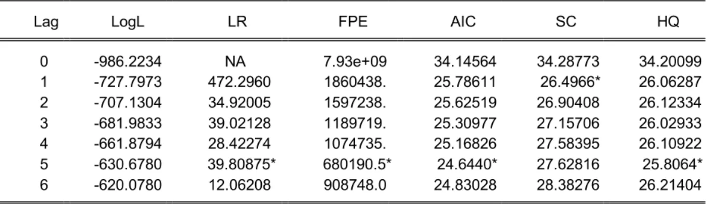
Table 3. VAR Lag Order Selection Criteria

Endogenous variables: GDP EXPEN REV DEBT Exogenous variables: C

Date: 05/08/10 Time: 14:07 Sample: 1 64

Included observations: 58

Lag LogL LR FPE AIC SC HQ

0 -986.2234 NA 7.93e+09 34.14564 34.28773 34.20099 1 -727.7973 472.2960 1860438. 25.78611 26.4966* 26.06287 2 -707.1304 34.92005 1597238. 25.62519 26.90408 26.12334 3 -681.9833 39.02128 1189719. 25.30977 27.15706 26.02933 4 -661.8794 28.42274 1074735. 25.16826 27.58395 26.10922 5 -630.6780 39.80875* 680190.5* 24.6440* 27.62816 25.8064* 6 -620.0780 12.06208 908748.0 24.83028 28.38276 26.21404 * indicates lag order selected by the criterion

LR: sequential modified LR test statistic (each test at 5% level) FPE: Final prediction error

AIC: Akaike information criterion SC: Schwarz information criterion HQ: Hannan-Quinn information criterion

Within this framework the Akaike and Hannan-Quinn information criteria selected 5 as the optimal number of lags. The result chosen by the Schwarz criterion, equal to 1 lag, could be neglected based on the economic theory: apparently, the changes in our variables have significant effects after several quarters or even years. An increase in the

expenditure, for example, cannot affect GDP only in the next quarter. This reasoning has determined my choice of 5 lags in the benchmark specification.

5.4.2.

Preliminary results

After running the model with 5 lags, all variables in levels, we obtained coefficients and t-statistics values for each of them. Most of the coefficients are non-significant at 5% level, but several are significant:

· Expenditure affects GDP after 5 quarters with a significant positive coefficient which is in line with economic theory

· Revenue affects GDP after 1 quarter with a significant positive coefficient · Revenue also affects Debt after 2 quarters with a significant positive coefficient The autocorrelation problem in the model is minor, serial correlation is observed only in the third time lag:

Table 4. VAR Residual Serial Correlation LM Tests

H0: no serial correlation at lag order h Sample: 1 64

Included observations: 59

Lags LM-Stat Prob

1 10.32041 0.8494 2 17.34637 0.3635 3 26.46379 0.0478 4 26.17741 0.0516 5 12.85328 0.6835 Probs from chi-square with 16 df.

Testing the roots of Characteristic Polynomial, one can find out that no root lies outside the unit circle, thus VAR satisfies the stability condition.

Following the methodology of Fatas & Mihov (2001), I used the Cholesky decomposition to identify impulse response functions. These functions show how GDP reacts to different shocks in expenditure, revenue and debt. For example, if the share of expenditure in GDP increases for one standard deviation, i.e. 2,53 percentage points, it will produce a maximum increase in GDP of 3464 million SEK after 8 quarters. The strong positive response of GDP to Revenue contradicts the underlying theory. According to theory, the tax increase should decline the GDP growth instead of stimulating it. Such measures prevent overheating in the economy and help to consolidate the budget. Thus we can conclude that this positive response is determined by one of the following reasons: the small sample size, non-stationary data or model misspecification.

Figure 3. Impulse response in the Benchmark model. -8000 -4000 0 4000 8000 12000 16000 20000 2 4 6 8 10 12 14 16 18 20 22 24 Response of GDP to EXPEN -8000 -4000 0 4000 8000 12000 16000 20000 2 4 6 8 10 12 14 16 18 20 22 24 Response of GDP to REV -8000 -4000 0 4000 8000 12000 16000 20000 2 4 6 8 10 12 14 16 18 20 22 24 Response of GDP to DEBT_SH

Response to Cholesky One S.D. Innovations ± 2 S.E.

The red dash lines in the graph indicate the ±2 SE standard bands around the impulse responses. In order to estimate the impulse response functions with the Cholesky decomposition one needs assume that changes in expenditure, revenue and debt variables do not have a contemporaneous effect on GDP. Apparently, such assumptions seem to be reasonable within the current framework of analysis.

Table 5. Variance decomposition of GDP

Period S.E. GDP EXPEN REV DEBT_SH

1 4665.753 100.0000 0.000000 0.000000 0.000000 2 7476.701 95.26235 0.005127 4.487601 0.244921 3 9791.571 93.09851 0.482365 6.173899 0.245227 4 11934.25 87.22999 2.161039 9.320962 1.288009 5 13888.53 76.73131 2.824092 16.72703 3.717567 6 16248.14 64.87332 4.452886 25.56436 5.109435 7 18693.80 54.29687 6.313979 32.43492 6.954229 8 21098.60 45.92429 7.651487 38.28579 8.138428 9 23394.49 40.34023 7.724875 43.47854 8.456361 10 25658.34 35.40119 7.584237 48.38673 8.627849

Variance decomposition indicates how much of a change in a variable is due to its own shock and how much is caused by shocks to other variables. The percentage of the effect of other shocks grows over time and often becomes prevailing. Variance decomposition combined with impulse response constitutes ‘Innovation accounting’.

The variance decomposition is directly related to the concept of exogeneity. There are three types of exogeneity: weak, strong and super exogeneity. The former two are statistical and the latter – causal. According to the definition, if a shock in a variable can explain most of the forecast error variance of the sequence GDP at all forecast horizons, then GDP is endogenous. Since within 20 lags almost 75 per cent of GDP variance is explained by the other three variables, GDP can be referred to as an endogenous variable. The revenue variable has the largest effect on the changes in GDP, within 20 lags it

explains more than 60 per cent of GDP fluctuations. Nevertheless, Hendry (2004) emphasizes the difference between the notions of exogeneity and causality. The latter is considered in the next section.

Granger causality test

A simple correlation coefficient is typically not sufficient for identifying the causation between two variables. The Granger (1969) approach to the question of whether X causes Y is to investigate if X values provide statistically significant information about future values of Y. If adding lagged values of X one can improve the explanation of Y, than Y is said to be Granger-caused by X. It is important to mention that the statement “ X Granger causes Y” does not mean that Y is the effect or the result of X. Granger causality can be a measure of precedence and information content. Meanwhile it does not indicate causality in the more common use of the term.

Table 6. Pairwise Granger Causality Tests (1)

Sample: 1 64 Lags: 5

Null Hypothesis: Obs F-Statistic Probability EXPEN does not Granger Cause GDP 59 1.66010 0.16244 GDP does not Granger Cause EXPEN 0.74612 0.59292 REV does not Granger Cause GDP 59 2.39290 0.05126 GDP does not Granger Cause REV 0.36818 0.86788 DEBT_SH does not Granger Cause GDP 59 0.85050 0.52107 GDP does not Granger Cause DEBT_SH 1.63972 0.16762

According to the estimates presented in the table, none of three policy variables Granger-cause GDP changes. The revenue as a share of GDP can Granger cause GDP growth only with 10 % confident interval. So in case of this model one can observe the difference between exogeneity and causality: GDP is endogenous to revenue, expenditure and debt, but is not Granger caused by any of these variables.

Non-stationarity might be a potential source of the model’s problems. This is why we test the data for stationarity in the next section.

5.4.3.

Stationarity of the data.

The statistical properties of my data set are well characterized by the quote from Hendry (2004): “All modern macro-economies are non-stationary from both stochastic and deterministic changes, often modeled as integrated-cointegrated systems prone to intermittent structural breaks—sudden large changes, invariably unanticipated”. All the shocks to policy variables are presented in Fig.C1 in the Appendix. In order to identify main shocks and eliminate seasonal fluctuations, I applied Census X12 technique, which is discussed in details in Section 5.8. The results are presented in Fig. C2. One can observe significant positive expenditure shocks in the beginning of 1999 and late 2008. The

debt exhibited high volatility in 2008-2009, which is related to the turmoil in the financial markets.

In order to check the data for stationarity I ran the Augmented Dickey-Filler unit root test.

Table 1. Stationarity of GDP variables

Levels 1st _Difference

GDP, absolute value Non-stationary Stationary ln(GDPt) – ln (GDPt-1) Stationary Stationary GDP growth rate, compared

to the same quarter of the previous year

Non-stationary Stationary

It is important to mention that [ln(GDPt) – ln (GDPt-1)] is the same as GDP growth compared to the previous quarter.

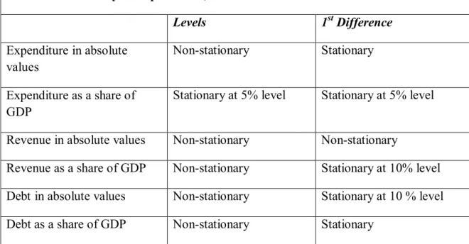
Table 2. Stationarity of Expenditure, Revenue and Debt variables

Levels 1st Difference Expenditure in absolute values Non-stationary Stationary Expenditure as a share of GDP

Stationary at 5% level Stationary at 5% level

Revenue in absolute values Non-stationary Non-stationary

Revenue as a share of GDP Non-stationary Stationary at 10% level Debt in absolute values Non-stationary Stationary at 10 % level Debt as a share of GDP Non-stationary Stationary

Concluding I can say that almost all the data is non-stationary when measured in levels and stationary when the first difference is taken.

5.5.

The model with first differences

Since the data series used in the Benchmark model were all non-stationary, it might be reasonable to test an alternative specification of the model with the following variables:

· The first difference of general government expenditure as a share of GDP (shortly – expenditure)

· The first difference of general government revenue as a share of GDP (shortly – revenue)

· The first difference of central government debt as a share of GDP (shortly – debt) The coefficients of this model should theoretically be the same as the coefficients for the benchmark model, since the first difference transformation does not affect them. Thus we can interpret these coefficients in the same manner as for the benchmark model, although the variables are different.

The choice of the optimal number of lags is trickier in this case since the Akaike criterion indicates 5 lags, the Schwarz criterion – 0 lags, whereas Hannan-Quinn offers the optimal number of 2 lags. Nevertheless, based on the economic theory I chose five lags as an optimal number.

The autocorrelation is present only for the third lag, so this minor problem can be neglected. According to the Pairwise Granger Causality Test, Revenue variable Granger causes GDP variable (both in first differences), all other variables do not Granger cause GDP.

There is no root of Characteristic Polynomial outside the unit circle, thus VAR satisfies the stability condition.

The impulse response is rather controversial: GDP responds to one standard deviation change in the first difference of expenditure (2.09 per cent of GDP) with a positive increase up to 1100 million SEK in the fourth quarter but then impulse fluctuates and change sign randomly. GDP also positively responds to an increase in Revenue and Debt variables.

Figure 4. Impulse response in the model with first differences

-4000 -2000 0 2000 4000 6000 1 2 3 4 5 6 7 8 9 10

Response of GDP_DIF to EXPEN_DIF

-4000 -2000 0 2000 4000 6000 1 2 3 4 5 6 7 8 9 10

Response of GDP_DIF to REV_DIF

-4000 -2000 0 2000 4000 6000 1 2 3 4 5 6 7 8 9 10

Response of GDP_DIF to DEBT_SH_DIF

Response to Cholesky One S.D. Innovations ± 2 S.E.

Combining this information with poor results of Variance decomposition (less that 30 per cent of GDP fluctuations are explained by shocks in the other variables) this allows us to conclude the small predictive and explanatory power of this model specification.

Another alternative specification included ln(GDPt) – ln (GDPt-1) as a measure of GDP growth, keeping all the rest variables the same. Unfortunately, the alternative model didn’t demonstrate any meaningful results. The GDP impulse response was randomly fluctuating along the horizontal axis, continuously changing the sign. Neither of three policy variables were Granger causing the GDP growth. Finally, according to variance decomposition, GDP growth was not endogenous variable and less than 35 per cent of its fluctuations were determined by the policy variables.

5.6.

The log model

Most of the researchers who analyzed fiscal policy results used all the variables in logs (see Blanchard & Perotti (2002), Giordano et al. (2008)). Log-linear model is a model that specifies a linear relationship among the log-transformed variables. This functional form has certain advantages over the linear one. Firstly, it helps to avoid biased growth estimates which can be present in the linear model. Parameters of the log-linear model are interpreted as elasticities. So such type of model is based on the assumption of constant elasticity over all values of the data set. It is also important to emphasize that R square values for linear and log-linear modification cannot be compared, since they are based on the estimations of the regressions which include different variables.

So in the next model specification I used: · The log of GDP level (shortly – GDP)

· The log of general government expenditure as a share of GDP (shortly – expenditure)

· The log of general government revenue as a share of GDP (shortly – revenue) · The log of central government debt as a share of GDP (shortly – debt)

The log function does not change significantly the stationary properties of the variables. It is also interesting to note that the results of the model do not change if we include log of absolute values of expenditure, revenue and debt.

The optimal number of lags is five. The GDP impulse response exhibits absolutely the same pattern as in the Benchmark model. There is a serial correlation in the third and the fourth lags. There are no roots lying outside the unit circle, so the model satisfies the stability condition.

Meanwhile there are significant changes in comparison with the first model.

Table 7. Pairwise Granger Causality Tests (2)

Sample: 1 64 Lags: 5

Null Hypothesis: Obs F-Statistic Probability

LN_REV does not Granger Cause LN_GDP 59 2.51984 0.04188 LN_GDP does not Granger Cause LN_REV 0.46939 0.79714 LN_EXP does not Granger Cause LN_GDP 59 1.70785 0.15089 LN_GDP does not Granger Cause LN_EXP 0.81162 0.54724 LN_DEBT_SH does not Granger Cause

LN_GDP 59 2.51888 0.04195

LN_GDP does not Granger Cause LN_DEBT_SH 2.82832 0.02565 Both Revenue and Debt Granger cause GDP changes. GDP is also better explained by the changes in policy variables according to Variance decomposition:

Table 8. Variance decomposition of ln_GDP

Period S.E. LN_GDP LN_EXP LN_REV LN_DEBT_SH 1 0.006953 100.0000 0.000000 0.000000 0.000000 2 0.010488 95.90704 0.027204 3.718710 0.347041 3 0.013232 93.54390 0.978035 4.313847 1.164223 4 0.015843 84.56309 4.027437 6.153166 5.256310 5 0.018247 70.48500 5.089826 12.45497 11.97021 6 0.021488 55.31109 7.332134 19.89952 17.45726 7 0.025250 42.18938 9.244843 25.82328 22.74250 8 0.029065 32.85891 10.48801 30.80618 25.84690 9 0.032686 27.12657 10.22462 35.50842 27.14039 10 0.036438 22.30760 9.598240 40.19710 27.89706

Thus one can conclude that the log-model has certain advantages over other modifications and provides the best results.

5.7.

Seasonality

Figure B in the Appendix clearly demonstrates that expenditure and revenue data is seasonally unadjusted. These seasonal variations in the main policy variables raise the possibility of spurious estimation from the VAR models. The method of seasonal smoothing proposed by Desai (2006) is to take average values for each year. Simply, expenditure value for the first quarter of 1994, for example, will be equal to the sum of expenditure values for 1994 divided by four. This way of handling the seasonality issue is not helpful, since it reduces the information set, but does not provide real seasonally adjusted data.

Another way of handling the problem is to use the Hodrick-Prescott (HP) Filter - a smoothing technique that is widely used among macroeconomists to obtain a smooth estimate of the long-term trend component of a series. The method was first used in a working paper by Hodrick & Prescott (1997) to analyze postwar U.S. business cycles. HP is a two-sided linear filter that computes the smoothed series Y*t of Yt by minimizing the variance of Yt around Y*t, subject to a penalty that constrains the second difference of Y*t. It includes a Lambda parameter which controls the smoothness of the series standard deviation. The larger is the Lambda, the smoother is the deviation. According to the Hodrick & Prescott (1997) methodology, the rule of thumb is: Lambda=100*(number of periods in a year)^2, thus for our quarterly data Lambda=100*4^2=1600.

I applied the HP filter to the Revenue and Expenditure, both measured as a share of GDP. Comparative graphs for de-trended data are presented in Appendix, Fig.D1 and Fig.E1. Then I tested a VAR model, which included GDP in levels and expenditure, revenue and debt all measured as shares of GDP8. Based on the Schwarz information criterion, the optimal number of lags was chosen to be 4.

The impulse response of GDP to shocks in the policy variables has changed considerably.

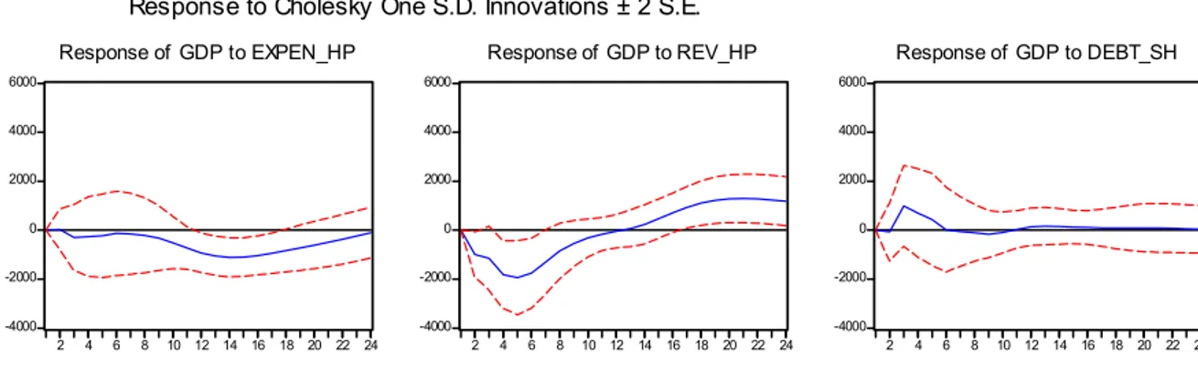
Figure 5. Impulse response in the model with HP-filter seasonal adjustment -4000 -2000 0 2000 4000 6000 2 4 6 8 10 12 14 16 18 20 22 24 Response of GDP to EXPEN_HP -4000 -2000 0 2000 4000 6000 2 4 6 8 10 12 14 16 18 20 22 24 Response of GDP to REV_HP -4000 -2000 0 2000 4000 6000 2 4 6 8 10 12 14 16 18 20 22 24 Response of GDP to DEBT_SH Response to Cholesky One S.D. Innovations ± 2 S.E.

The coefficients in VAR for revenue became significant or nearly significant, but they have meaningless signs: in periods (t-1) and (t-3) revenue has negative coefficients, whereas in periods (t-2) and (t-4) it has a positive coefficient. Also a severe autocorrelation problem is present in the model in all 4 lags. Finally, neither of policy variables Granger causes GDP.

Consequently I can conclude that the HP-filter does not improve the model results. In order to achieve better estimates, one needs to employ more comprehensive seasonal adjustment methods.

The last adjustment technique which I employed to eliminate seasonal fluctuations in the expenditure and revenue variables was Census X12 method, developed by the U.S. Census Bureau. The procedure estimates and removes seasonal factors from data series using comprehensive seasonal and moving averages tools. In comparison with the HP-filter this procedure provides us with arguably more informative results (see Fig. D2 and Fig. E2 in the Appendix). Employing this data I tested the same model with GDP in levels and three policy variables measured as shares of GDP. Based on the Akaike criterion I chose 5 lags to analyze and obtained the results which are similar to the model with seasonally unadjusted data. Nevertheless, there are certain differences. GDP responds to the expenditure shock in a different manner.

Figure 6. Impulse response in the model with X12 seasonal adjustment

-5000 0 5000 10000 15000 20000 2 4 6 8 10 12 14 16 18 20 22 24 Response of GDP to EXPEN_SA -5000 0 5000 10000 15000 20000 2 4 6 8 10 12 14 16 18 20 22 24 Response of GDP to REV_SA -5000 0 5000 10000 15000 20000 2 4 6 8 10 12 14 16 18 20 22 24 Response of GDP to DEBT_SH

Response to Cholesky One S.D. Innovations ± 2 S.E.

As one can see from the charts, in the first three periods GDP has a small negative responsive, but starting from the fourth quarter the response becomes strongly positive,

peaking in the 8th _{period with the value 2715 million SEK (which is lower that the} response of GDP in the benchmark model).

The model has no autocorrelation. None of policy variables Granger cause GDP. According to variance decomposition, GDP is endogenous variable, since almost 70 per cent of its fluctuations are explained by the policy variable.

Concluding, I can say that none of seasonal adjustment techniques has helped to improve the model considerably. Apparently, the seasonality issue is not the cause of estimation mistakes.

5.8.

Potential sources of problems

It is important to indicate the potential sources of divergence between the model results and the macroeconomic theory. The problems are:

1. A small sample size, which was determined by the intention to analyze the current business cycle fluctuations.

2. Multicollinearity problem is almost inevitable when one conducts this sort of analysis. It results in low t-values for regression coefficients, which tend to be insignificant. The F-values are usually high, meaning that it is not possible to reject the hypothesis that all variables may be statistically significant on the basis of a standard F-test (Gujarati, 2004).

3. Better results can be arguably obtained by implementing a different methodology for the shock estimation. For example, Blanchard & Perotti (2002) exploited decision lags in fiscal policymaking and used information about the elasticity of fiscal variables to economic activity, which allows to identify the automatic response of fiscal policy. This methodology is rarely used for studying countries different from U.S., because of the limited availability of quarterly public finance data (Giordano et al., 2008)

4. At first sight, the reaction of GDP to the revenue growth in the benchmark model contradicts the theory: it reacts to a positive shock in revenue with a strong and continuous positive increase. Meanwhile Giordano et al. (2008) obtained very similar results. In their benchmark model GDP (net of government consumption) grows in response to a positive government revenue shock with the maximum increase in the 5th quarter. They consider this effect as transitory and irrelevant, although it is present in different model specifications. This can be an issue for a further in-depth research.

Thus the VAR model re-approved the mechanisms which were described in the qualitative analysis (Section 4). It also contributed some approximations for the response functions and the estimations of the GDP increase in response to expansionary fiscal

6. Conclusions

The governments of many countries around the world implemented various fiscal measures in response to the economic downturn of 2008-2010. The Swedish government also introduced a significant fiscal package. And, although the economic downturn had unprecedented scale, intensity and duration, Sweden has successfully coped with the crisis. It is worth mentioning that this success became possible only due to close cooperation between fiscal and monetary policy. An accommodative monetary policy provided by Riksbank was a necessary precondition for effective fiscal expansionary policy.

This paper analyzed the fiscal policy in Sweden using quantitative and qualitative methods. A review of currently implemented stabilization measures has been presented along with the analysis based upon theory and recent economic developments. The quantitative part of the paper describes a 4-variable structural VAR model which includes GDP, general government expenditure and revenue and central government debt. Based on this model the effects of shocks of policy variables on GDP were estimated for the period 1994-2009.

The VAR model in different specifications demonstrates a positive response of GDP to an increase in government expenditure. If the share of expenditure in GDP increases for one standard deviation, i.e., 2,53 percentage points, it will produce a maximum increase in GDP of 3464 million SEK after 8 quarters. GDP also grows in response to a positive shock in the central government debt, which is in line with the macroeconomic theory of expansionary fiscal policy. The positive response to an increase of revenue is somewhat contradictory, meanwhile similar results were obtained by other researchers.

Different methods were used in this paper to improve the model’s explanatory power: the first difference modification, the log transformation and seasonal adjustment for revenue and expenditure variables. The log model has certain advantages over the other modifications: both revenue and debt Granger-cause GDP changes. Moreover GDP dynamics is better explained by the changes in policy variables according to the variance decomposition in the log model.

Some of the possible ways to improve the model are by using a larger sample of data and by introducing another way of shock estimation. Nevertheless, it is essential to treat the VAR models estimations cautiously, keeping in mind the underlying restrictions and assumptions

It is important to emphasize that the global recession is not over yet and the governments of different countries have yet to recover their economies and stimulate growth. Studying the experiences of those countries which have managed to successfully overcome the crisis, one can get a good example of an effective fiscal policy. The Swedish government efficiently met the challenges of the crisis, this is why it is helpful to investigate the measures and policies which they have used. It is a long-term task for economists to assist policymakers in strategic decision-making process by providing accurate and reliable research data. Hopefully, the results of this paper will contribute to the academic research of fiscal policy.