Using geospatial techniques and remote sensing to reduce the number of soil salinity samples

(1)

Using Geospatial Techniques and Remote Sensing to Reduce the

Number of Soil Salinity Samples

Ahmed A. Eldeiry1

Department of Civil and Environmental Engineering, Colorado State University, 80523, Luis A. García

College of Engineering and Mathematical Sciences, University of Vermont, Burlington, VT 05405. Abstract. Geostatistical techniques and remote sensing are used in this study to help reduce the

number of soil salinity samples needed for mapping soil salinity. Two datasets were collected in alfalfa and corn fields and satellite images with different spatial and spectral resolutions from Ikonos, Landsat, and Aster were acquired and processed. Generalized least squares (GLS) was used to regress the collected soil salinity samples with the selected bands; and ordinary kriging was used to krig the residuals of the GLS model. Variograms were used as indictors for using the proper number of samples needed for kriging in order to map soil salinity. The objectives of this study are: 1) to utilize the variograms to help reduce the number of samples needed for mapping soil salinity; 2) to compare different cover types (alfalfa and corn) as well as compare different satellite images in capturing the variation of soil salinity. The results of this study show that the variograms can be used as a good indicator to significantly reduce the number of samples needed for mapping soil salinity. It was determined that corn fields capture more varia-tion in soil salinity than alfalfa fields. Among the different satellite images used, the IKONOS images performed the best.

1. Introduction

Soil salinity refers to the presence in soil and water of various electrolytic minerals solutes in concentrations that are harmful to many agricultural crops (Hillel 2000). Salts decrease the availability of water to plants due to the increase in the osmotic potential. Therefore, they have a direct adverse effect on the plant metabolism (Douaik et al. 2004). Mapping and assessing soil salinity is the first step towards salinity manage-ment. Mapping soil salinity requires considerable effort in field sampling, therefore, the selection of an optimal sampling design is important. Sampling incorporates concepts of survey intensity, spatial variability, mapping scale, and is usually the most costly and labor-intensive aspect of a soil survey (Webster and Oliver 1990). In a conventional soil survey, surveyors subjectively select sampling sites to support their mental predic-tive model of soil occurrence, a so-called free survey (White 1997). Such designs are purposive and non-random, and do not provide statistical estimates. By contrast, a pe-dometric, which is used in this study, soil survey (McBratney et al. 2000) aims at statis-tical modeling of soil cover, including uncertainty about the predictions using objective techniques.

Geostatistical methods for soil salinity sampling and mapping provide a means to study the heterogeneity of the spatial distribution of soil salinity (Pozdnyakova and Zhang 1999). They have been recognized as a powerful tool in the selection of the sampling design and in the mapping of soil properties (Bouma 1984; Wilding 1984). In geostatistical theory, the range of the variogram is the maximum distance between cor-related measurements (Journel and Huijbregts 1978; Warrick et al. 1986). This means that samples separated at smaller distances than the range of the variogram are

1_{Integrated Decision Support Group, Department of Civil and Environmental Engineering, Colorado State}

(2)

ly not needed (Nielsen et al. 1983). Therefore, the range of variograms can be an effec-tive criterion for the selection of a sampling design in mapping soil salinity (Utset et al. 1998). Many investigators have studied the use of variograms to improve the estimation of the number of samples needed (Davis and Borgman 1982; Myers 1991). Given a col-lection of data, a variogram reveals the type of spatial structure inherent to a spatial phenomenon. In addition, the variogram reveals the amount of noise present in the data, known commonly as the nugget (Carr et al. 1985). Variograms have been widely used to analyze spatial structures in ecology (Phillips 1985, Robertson 1987). In addition, variograms of electrical conductivity can be useful toGLS in determining the spacing between soil samples for laboratory electrical conductivity determination (Utset et al. 1998). Several studies have shown that an increase in precision can be achieved with a smaller sample size when using kriging as compared to sampling techniques that as-sume spatial independence (McBratney and Webster 1983; Di et al. 1989; Chung et al. 1995). Sampling costs can be dramatically reduced and estimation can be significantly improved by using Cokriging (Pozdnyakova and Zhang 1999).

Remote sensing of surface features has been used intensively to identify and map salt affected areas (Robbins and Wiegand 1990). Multispectral data acquired from plat-forms such as Landsat, SPOT, and the Indian Remote Sensing (IRS) series of satellites have been found useful in detecting, mapping, and monitoring salt affected soils (Dwivedi and Rao 1992). The location of each field soil salinity sample should be over-laid on a satellite image to obtain the pixel intensity. Then, if the field data are spatially correlated with the intensity of the remotely sensed image, a model describing the spa-tial continuity could be developed (Cliff and Ord 1981). Eldeiry and Garcia (2008a,b; 2010) used geostatistical techniques with remote sensing data to estimate soil salinity. Eldeiry et al. (2008) developed a strategy to reduce the number of soil salinity samples needed for mapping soil salinity. The strategy includes using spatial modeling tech-niques, remote sensing and field data. Wiegand et al. (1994) developed a procedure for using soil salinity, plant information, and digitized color infrared aerial photography and videography to help determine soil salinity. Color and thermal infrared aerial pho-tography as well as spectral image interpretation techniques have been used for map-ping surface land salinity (Spies and Woodgate 2004).

The practical purpose of this study is to establish a reliable field sampling strategy to detect temporal changes of soil salinity on alfalfa and corn fields. The approach pre-sented in this study involves integrating remotely sensed data, geostatistical techniques, to reduce the number of soil salinity samples needed. The cross-correlation between the field soil salinity data and the different satellite images was established based on using crop cover type reflection as an indicator of soil salinity. Two main datasets were col-lected in alfalfa and corn fields, the methodology was also applied to nine data subsets generated randomly from the two main datasets ranging from 10% to 90% of the total number of observations in 10% increments. The subsets were used to evaluate the in-fluence of sample size on capturing the variability within the fields. The stepwise pro-cedure was used to select the bands from the satellite images that best correlated with the collected soil salinity data. Generalized least squares (GLS) was used to regress the collected soil salinity data with the selected bands of the satellite images. The residuals of the GLS model were checked for autocorrelation and kriged using ordinary kriging. The generated surface of the kriged residuals was added to the surface developed using the GLS model to form a regression kriging surface. When kriging the residuals, the range of the variogram was used to assess the maximum distance at which samples are

(3)

correlated. In each case, the estimated values were compared with the collected data us-ing several statistical measures. The methodology presented in this study has the poten-tial to significantly reduce the number of samples that are collected and therefore the cost associated with the samples, especially for projects that last multiple years or re-quire multiple sampling events in the same area.

2. Materials and Methods

2.1. The Study Area

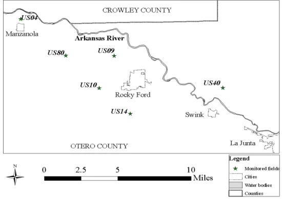
The study area is located in southeastern Colorado, near the town of La Junta (Fig-ure 1). Fields in this area are planted with corn, alfalfa, wheat, onions, cantaloupe and other vegetables, and are irrigated by a variety of systems including a mixture of border and basin, center pivots and a few drip systems. Salinity levels in the irrigation canal systems along the river increase from 300 ppm total dissolved solids (TDS) near Pueblo to over 4,000 ppm at the Colorado-Kansas border (Gates et al. 2012). In this area, Colo-rado State University (CSU) has conducted an intensive field data collection effort that includes water table elevation, irrigation amounts, crop yields, rainfall data, and soil sa-linity data. This study deals with the soil sasa-linity data that was collected in intensively monitored fields where alfalfa and corn were planted during 2001 and 2004 and the fields were covered by a number of satellite images.

Figure 1. The study area with the location of corn and alfalfa fields.

2.2. Data Collection

Soil salinity was measured in the fields using an EM-38 electromagnetic probe. The EM-38 takes vertical and horizontal readings that can be converted to soil salinity esti-mates (Eldeiry and Garcia 2008). The EM-38 can cover large areas quickly without ground electrodes and provides depths of exploration of 1.5 meters and 0.75 meters in the vertical and horizontal directions, respectively. Two soil salinity sample datasets were collected using EM-38 probes. The first dataset, consisting of 326 points in four corn fields in 2001 (US09, US10, US40, and US80), was used with ASTER,

(4)

LAND-SAT 7 and IKONOS satellite images. The second dataset consists of 256 points in four alfalfa fields in 2004 (US04, US09, US10, and US14), and was used with LANDSAT 5 and IKONOS satellite images. Table 1 characterizes the intensively monitored fields planted with corn and alfalfa used in this study. The table shows that there is a large range of soil salinity in these fields from 2.5 to 20.7 dS/m. The use of reliable maps is advantageous because of the large variation in soil salinity. The theoretical require-ments for using kriging and spatial statistics may be inappropriate depending on the types of spatial variations.

Table 1. The description of the alfalfa and the corn fields that were monitored.

Field Area (hectare) Soil salinity range Irrigation system

Corn fields 2001

US09 21.0 2.5 – 3.7 Surface (gated pipes)

US80 3.3 2.7 – 11.7 Surface (siphons)

Alfalfa fields 2004

US04 105.6 2.7 – 20.7 Center pivot sprinkler

2.3. Satellite Images Description and Processing

Four satellite image types were evaluated for their ability to estimate soil salinity. The Advanced Spaceborne Thermal Emission and Reflection Radiometer (ASTER) (Yamaguchi et al. 1998) sensor is an imaging instrument flown on the Terra satellite launched in December 1999. ASTER is a cooperative effort between NASA and Japan's Ministry of Economy and has been designed to acquire land surface tempera-ture, emissivity, reflectance, and elevation data. An ASTER scene covers an area of ap-proximately 60 km by 60 km and consists of 14 bands of data: three bands in the visible and near infrared (VNIR) with 15 m resolution, six bands in the short wave (SWIR) with 30 m resolution, and five thermal bands (TIR) with 90 m resolution. The ASTER image was acquired on August 16th, 2001 and all bands were resampled to 30 m resolu-tion. LANDSAT 7 images have three visible bands (blue, green, and red), one near in-frared band (NIR) and two shortwave inin-frared bands (MIR-1, MIR-2) at 30 m resolu-tion; a thermal infrared band (TIR) at 60 m resoluresolu-tion; and a panchromatic (PAN) band with 15 m resolution. The LANDSAT 7 image was acquired on July 8th, 2001 and was also resampled to 30 m resolution. IKONOS images have three bands visible (blue, green, and red) and one in the near infrared (NIR) with a resolution of 4 m, and a pan-chromatic band with 1 m resolution. The IKONOS image was acquired on July 11th, 2001. The LANDSAT 5 images contain seven bands, including three visible bands (blue, green, and red) with 30 m resolution, two NIR bands (band 4 and band 5) with 30 m resolution, one thermal band (band 6) with 120 m resolution, and a Mid IR (band 7) with 30 m resolution. The LANDSAT 5 image was obtained on August 9th, 2004. The four satellite images are highly variable in spectral and spatial resolution, with a range of four to fourteen spectral bands and 1 m to 120 m spatial resolution. This vari-ability provides the opportunity to explore the use of spatial and spectral resolution for predicting soil salinity.

(5)

The normalized difference vegetation index (NDVI) was added to the bands of the images. The NDVI uses the contrast between red and infrared reflectance as an indica-tor of vegetation cover and vigor. The NDVI was developed to provide an indication of the amount of vegetation (Wiegand et al. 1994, Hill and Donald 2003).

2.4. Using the GLS Model

Generalized Least Squares (GLS) is an extension of the Oeneralized least squares OLS method, that allows efficient estimation of β when correlations is present among the error terms of the model, as long as the form of correlation is known independently of the data. To handle heteroscedasticity when the error terms are uncorrelated with each other, GLS minimizes a weighted analogue to the sum of squared residuals from OLS regression, where the weight for the ith_{case is inversely proportional to var(ε}

i).

This special case of GLS is called "weighted least squares". The GLS solution to esti-mation problem is y Ω X X) Ω (X βˆ ₌ T −1 −1 T −1 ₍₁₎

Where Ω is the covariance matrix of the errors. GLS can be viewed as applying a line-ar transformation to the data so that the assumptions of OLS line-are met for the trans-formed data. For GLS to be applied, the covariance structure of the errors must be known up to a multiplicative constant.

The predicted responses were then subtracted from the observed responses to obtain the residuals. Examining the residuals is a key part of all statistical modeling diagnos-tics since residuals indicate whether the chosen model is appropriate. Therefore, the re-siduals derived from the GLS model inspected for normality and spatial autocorrela-tion.

When applying an GLS model, if any band in the selected subset shows a p-value <0.05, this band is removed and the GLS model is applied again. This procedure is re-peated until each individual band in the subset of bands has a p-value <0.05 to guaran-tee that the selected bands have strong cross-correlation with the collected soil salinity data.

Examining the residuals is a key part of all statistical modeling diagnostics since re-siduals indicate whether the chosen model is appropriate. Therefore, the rere-siduals de-rived from the GLS model were inspected for normality, homogeneity and spatial auto-correlation. The assumption of the residuals is that they should have a normal distribu-tion and no spatial autocorreladistribu-tion. If the GLS model residuals did not satisfy this as-sumption, then the residuals were kriged and added to the generated surface using the GLS model to produce the modified residual kriged model. Normality of the GLS model was inspected by evaluating the histogram of residuals and the residuals versus the quantiles of a standard normal distribution. Homogeneity was inspected by evaluat-ing the residuals versus the weight of the residuals and the residuals versus the estimat-ed soil salinity. The autocorrelation was inspectestimat-ed by evaluating a Moran’s I p-value >0.05.

2.5. Using Variograms

The spatial structure of the residuals from the GLS regression models were ana-lyzed for spatial continuity using the variogram. The sample variogram, γˆ

( )

h is esti-mated using the following equation:

(6)

( )

_{( )}

_∑

( )

[

( ) (

)

]

= + − = N h i i i s h s h N h 1 2 ˆ ˆ 2 1 ˆ _ε _ε γ (2)

where εˆ

( )

s_i and εˆ

(

s_i +h

)

are the estimated residuals from the regression models at lo-cations s and _i si + , a location separated by distance h; N(h) is the total number of h

pairs of samples separated by distance h. The empirical variogram, which is a plot of the values of γˆ

( )

h as a function of h, gives information on the spatial dependency of the variable. Exponential, gaussian and spherical models were fitted to the sample variograms using a weighted least squares method (Robertson 1987).

For each dataset a variogram was generated to evaluate the maximum correlation distance between soil salinity samples. Each time a given dataset was reduced by 10%, the range of the variogram, which identifies the maximum distance between the corre-lated points and how well it fit, provided an indication as to whether the sample points that were removed were needed. The variogram model with the smallest AICC was se-lected to describe the spatial dependencies in the salinity data. The best-fit variogram model was used to describe the spatial continuity in estimating the kriging weights. The kriged residual surface was generated for each data subset and combined with the GLS surface. If the residuals were spatially auto correlated, ordinary kriging was used to model the spatial continuity of the errors in predicting soil salinity in the fields. At every spatial location so, where a soil salinity sample was not collected, estimates of the true unknown residuals, ε

( )

s_o , were obtained using a weighted linear combination of the available soil salinity samples at spatial locations, si, as follows:

( )

_∑

( )

= = n i i i o w s s 1 ˆ ˆ ε ε (3)

where the set of weights _{w takes into consideration the distances between soil salinity}_i sample locations and spatial continuity or clustering between the soil salinity samples.

2.6. Model Evaluation Measures

The effectiveness of the final models was evaluated using a goodness-of-prediction statistic, G (Agterberg 1984, Kravchenka and Bullock 1999, Guisan and Zimmermann 2000, Schloeder et al., 2001). The G-value measures how effective a prediction might be relative to something that could have been derived by using the sample mean (Ag-terberg 1984):

[

]

[

]

_⎟⎟⎠⎞ ⎜⎜⎝ ⎛ ⎭ ⎬ ⎫ ⎩ ⎨ ⎧ ₋ ₋ − =

∑

= = n i i n i i i Z Z Z Z G 1 2 1 2 ˆ 1 , (4)

where Z is the observed value of the i_i th observation, Zˆ_i is the estimated value of the ith observation, and Z is the sample mean. A G-value equal to 1 indicates perfect predic-tion, a positive value indicates a more reliable model than if one had used the sample mean, a negative value indicates a less reliable model than if one had used the sample mean, and a value of zero indicates that the sample mean should be used to estimate Z.

The standardized mean squared error (SMSE) was used to test the null hypothesis of equal variance (Hevesi et al. 1992):

( )

(

)

∑

= = n i i i s z s n 1 var ˆ ˆ 1 SMSE ε (5)

(7)

where _εˆ

( ) ( ) ( )

s_i ₌

(

z s_i ₋zˆ s_i

)

is the true error, and var

(

zˆ

( )

s_i

)

is the estimated variance obtained.

The estimated variances were assumed to be consistent with the true errors if the SMSE falls within the interval

[

1±2

( )

2 n −1/2

]

(Hevesi et al. 1992). In addition to the G-value and SMSE, the standard deviation and coefficient of variation were also tested through the cross-validation process. Visual measures were also used for the observed and estimated data using all datasets for all images. X-Y scatter plots were used to dis-play the scatter of the data and histogram plots were used to disdis-play the distribution; the maps of the estimated data generated from remote sensing were compared with the ob-served data.

2.7. Model Validation

The modified residual kriging model was validated using a variety of different da-tasets to verify that it produced generally good results. For this study, the modified re-sidual kriging model was validated in two different ways: 1) for each dataset, one field data subset was removed and estimated using the rest of the data for the other fields. This procedure was repeated for each field in the 2001 and 2004 datasets with each of the satellite images; and 2) cross-validation (Efron and Tibshrani 1993) was used to es-timate the prediction error for soil salinity. The data were split into 10 parts and for each part the modified residual kriging model was fitted to the remaining nine subsets of the data. The fitted model was then used to predict the part of the data removed be-fore the modeling process. This process was repeated 10 times so that each sample subset was excluded from the model fitting step and a corresponding model response estimated. Repeating this process over many excluded subsets allows an assessment of the variability of the prediction error. The cross-validation procedures used in this study based on Stone (1974) and Geisser (1975) has become a popular method of assessing model accuracy and prediction.

3. Results and Analysis

3.1. Evaluating the GLS Model

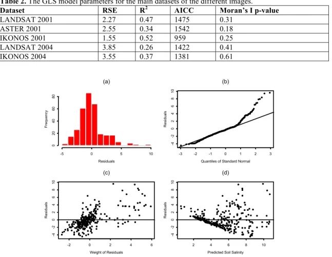
Table 2 shows the residual standard errors (RSE), R2, AICC, and Moran’s I p-values of the GLS model with the two main datasets for corn and alfalfa with the dif-ferent satellite images. Comparing corn to alfalfa, all RSE, R2, and AICC show that corn produces better results than alfalfa. That is clear from the RSE parameter where the corn RSE values are less compared to those of alfalfa. Also R2 values for corn are higher than the corresponding values of alfalfa. Only the AICC value for the 2004 LANDSAT image with alfalfa is slightly less than that of the 2001 LANDSAT image while the AICC of the 2001 IKONOS image is significantly less than that of the 2004 IKONOS image when alfalfa is used. The p-value of each individual set is larger than 0.05, which indicates an autocorrelation among the residuals. Figure 2 is a graphical in-spection of the residuals of the GLS model using observed soil salinity data in conjunc-tion with the LANDSAT 7 image. The two graphs at the top are used to inspect normal-ity while the two graphs at the bottom are used to inspect homogenenormal-ity. Figure 2a shows that the distribution is not exactly normally distributed but skewed to the right. Figure 2b (Q-Q graph) shows that the empirical quantiles are very close to the line be-tween the values of -3 to 1, and that the points start to deviate from the line for values greater than 1. The skewness of the histogram in Figure 2a and the deviation of the

(8)

points from the line in Figure 2b indicate that residuals are not normally distributed and not homogeneous. Figure 2c displays the residuals versus the weight of the residuals and it shows a pattern and some cluster in the distribution, while Figure 2d shows that the distribution of points is not scattered randomly about 0—both are signs that the re-siduals are not homogenous.

Table 2. The GLS model parameters for the main datasets of the different images.

Dataset RSE R2 AICC Moran’s I p-value

LANDSAT 2001 2.27 0.47 1475 0.31 ASTER 2001 2.55 0.34 1542 0.18 IKONOS 2001 1.55 0.52 959 0.25 LANDSAT 2004 3.85 0.26 1422 0.41 IKONOS 2004 3.55 0.37 1381 0.61 -5 0 5 10 0 20 40 60 80 Residuals Fr eq u en cy (a)

Quantiles of Standard Normal

Resid u als -3 -2 -1 0 1 2 3 -4 -2 0 2 4 6 8 10 (b) Weight of Residuals Resid u als -2 0 2 4 6 -4 -2 0 2 4 6 8 10 (c)

Predicted Soil Salinity

Resid u als 2 4 6 8 10 -4 -2 0 2 4 6 8 10 (d)

Figure 2. Inspection of the residuals of the GLS models for the LANDSAT 7 image with corn dataset

2001. (a) The histogram of residuals (b) The residuals versus the quantiles of standard normal (c) The re-siduals versus the weight of the rere-siduals (d) The rere-siduals versus the estimated soil salinity.

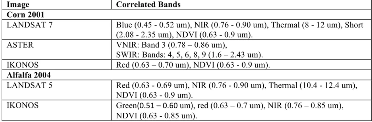
3.2. Correlated Bands

Table 3 shows the correlated bands of each image for each dataset where the p-value of each band is less than 0.05 to guarantee a correlation between the bands and the observed soil salinity. The most significant band that appears in all images with corn and alfalfa is the near infrared (NIR) band, except for the 2001 IKONOS image with corn. Among the three visible near infrared bands of ASTER, band 3 with a spec-tral resolution of 0.78-0.86 um has the same resolution of NIR bands of LANDSAT or IKONOS; therefore these two bands are similar. NDVI also appears in all images ex-cept in the ASTER image. Even though the NDVI does not appear in the ASTER im-age with corn, the VNIR band does appear and its spectral resolution is within the spec-tral resolution of the NDVI. This makes the NIR band and NDVI index the most prom-inent for both corn and alfalfa. The blue, thermal, and short bands appear in corn with LANDSAT 7 while the red band appears in alfalfa with LANDSAT 5. Some other bands such as red, green, and thermal appear occasionally in alfalfa or corn with differ-ent images.

(9)

Table 3. The correlated band combinations with the collected soil salinity data with different images for

datasets where p-value <0.05 of individual band.

Image Correlated Bands

Corn 2001

LANDSAT 7 Blue (0.45 - 0.52 um), NIR (0.76 - 0.90 um), Thermal (8 - 12 um), Short (2.08 - 2.35 um), NDVI (0.63 - 0.9 um).

ASTER VNIR: Band 3 (0.78 – 0.86 um),

SWIR: Bands: 4, 5, 6, 8, 9 (1.6 – 2.43 um). IKONOS Red (0.63 – 0.70 um), NDVI (0.63 - 0.9 um).

Alfalfa 2004

LANDSAT 5 Red (0.63 - 0.69 um), NIR (0.76 - 0.90 um), Thermal (10.4 - 12.4 um), NDVI (0.63 - 0.9 um).

IKONOS Green(0.51 – 0.60 um), red (0.63 – 0.7 um), NIR (0.76 – 0.85 um), NDVI (0.63 - 0.85 um).

3.3. Variograms and Number of Soil Salinity Samples

The variograms for the various fields were constructed using all the data as well as each of the data subset for each individual satellite image. Figure 3 shows an example of the different variograms used in the kriged residuals technique using the LANDSAT 7 image. Figure 3 shows that there is no significant difference in fitting the variograms until 40% of the data or below is used. Below 40% of the data, the variograms do not fit. These results show that there are a significant number of soil salinity samples that can be removed without having a large impact on the accuracy of the interpolation technique. This means that 326 soil salinity samples collected in corn fields can be re-duced to 130 soil salinity samples without significant impact on the accuracy of the in-terpolation technique.

In general, all the AICC values for corn are smaller than those of alfalfa for all da-tasets and satellite images. All the AICC values for LANDSAT 7 and IKONOS with corn are less than the corresponding values of the LANDSAT 5 and IKONOS with al-falfa. Comparing the results from different satellite images, the AICC values of the ASTER image are the largest and the IKONOS image values are the smallest. The AICC values of LANDSAT 5 and IKONOS images with alfalfa are higher than the cor-responding values of the IKONOS image. The results of this table also support the re-sults from Figure 3 where the variogram does not fit well with the small sub datasets. The AICC values obtained using corn fields were better than those obtained in alfalfa fields. In addition, IKONOS images provide better estimates than LANDSAT or AS-TER images. Based on the results from Figure 3, the exponential model is slightly bet-ter than the gaussian and the spherical models; therefore it was used in this study.

3.4. Comparison of the Estimated Data Using the Five Satellite Images

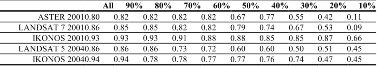
Table 4 shows the G-values of the estimated soil salinity for all datasets with all images. Most G-values of the LANDSAT 7 and IKONOS images with corn are higher than the corresponding G-values of alfalfa. IKONOS images in both corn and alfalfa have the highest G-values compared to LANDSAT and ASTER images. LANDSAT and ASTER images almost have similar values. As the datasets get smaller the G-values get smaller, which supports the results of the variograms where for datasets of less than 40% have a poor fit.

(10)

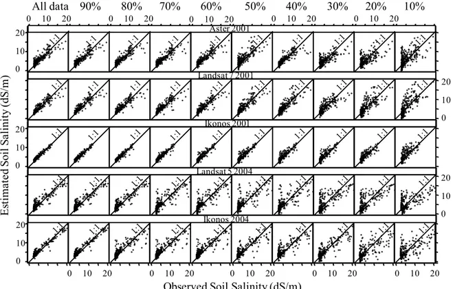
Figure 4 shows the x-y plots for all images and datasets. The x-y plots show that there is a good trend between the estimated and observed data when using all the data. The IKONOS images for both the corn and alfalfa fields have the best correlation with the observed soil salinity, second best was LANDSAT 7 with corn, then ASTER with corn, and last LANDSAT 5 with alfalfa. There is a strong similarity between the x-y figures and the variogram figures in that below 40% of the data there is more scatter in the x-y plots associated with the poor fit in the corresponding variograms. As the size of the datasets is reduced the scatter in the x-y plots increases and the range of the his-tograms of the estimated data deviates from the range of the hishis-tograms of the observed data. xp yp 0 50 100 150 200 250 2 3 4 5 6

Fitting variogram models (all data)

xp yp 0 50 100 150 200 250 2 3 4 5 6

Fitting variogram models (90% of data)

xp yp 0 50 100 150 200 250 2 3 4 5 6

xp yp 0 50 100 150 200 250 1 2 3 4 5 6

xp yp 0 50 100 150 200 250 2 3 4 5 6

xp yp 0 50 100 150 200 250 1 2 3 4 5 6

xp yp 0 50 100 150 200 250 1 2 3 4 5

xp yp 0 50 100 150 200 250 1 2 3 4 5 6

xp yp 0 50 100 150 200 250 0 1 2 3 4 5 6

Exponential Spherical Gaussian 0 50 100 150 200 250 2 3 4 0 50 100 150 200 250 0 50 100 150 200 250 0 50 100 150 200 250 2 3 4 0 50 100 150 200 250 0 50 100 150 200 250 0 50 100 150 200 250 1 2 3 4 5 0 50 100 150 200 250 0 50 100 150 200 250 0 5 10 15 2 3 4 1 2 3 4 1 2 3 4 5 1 2 3 4 5 1 2 3 4 5 0 1 2 3 4 5 6 0 50 100 150 200 250

Variogram models (all data)

Distance h (m) Variogram models (70% of data)

Distance h (m)

Variogram models (90%of data)

Distance h (m)

Variogram models (80% of data)

Distance h (m) γ( h) γ( h) γ( h) γ( h) γ( h) γ( h) γ( h) γ( h) γ( h) γ( h)

Figure 3. Variogram models for the LANDSAT 7 image for all datasets for corn fields.

Table 4. G-values of the estimated soil salinity for all datasets for all images.

All 90% 80% 70% 60% 50% 40% 30% 20% 10% ASTER 20010.80 0.82 0.82 0.82 0.82 0.67 0.77 0.55 0.42 0.11 LANDSAT 7 20010.86 0.85 0.85 0.82 0.82 0.79 0.74 0.67 0.53 0.09 IKONOS 20010.93 0.93 0.93 0.91 0.88 0.88 0.85 0.85 0.87 0.66 LANDSAT 5 20040.86 0.86 0.86 0.73 0.72 0.60 0.60 0.50 0.51 0.45 IKONOS 20040.94 0.94 0.78 0.78 0.77 0.77 0.76 0.74 0.47 0.45

(11)

0 5 10 15 20 num 0 5 10 15 20 num 0 5 10 15 20 num 0 5 10 15 20 num 0 5 10 15 20 num 0 5 10 15 20 num 0 5 10 15 20 num 0 5 10 15 20 num 0 5 10 15 20 num 0 5 10 15 20 num 0 5 10 15 20 Obs P red 0 5 10 15 20 num 0 5 10 15 20 num 0 5 10 15 20 num 0 5 10 15 20 num 0 5 10 15 20 num 0 5 10 15 20 num 0 5 10 15 20 num 0 5 10 15 20 num 0 5 10 15 20 num 0 5 10 15 20 num 0 5 10 15 20 OBS P red 0 5 10 15 20 num 0 5 10 15 20 num 0 5 10 15 20 num 0 5 10 15 20 num 0 5 10 15 20 num 0 5 10 15 20 num 0 5 10 15 20 num 0 5 10 15 20 num 0 5 10 15 20 num 0 5 10 15 20 num 0 5 10 15 20 Obs P red 0 5 10 15 20 num 0 5 10 15 20 num 0 5 10 15 20 num 0 5 10 15 20 num 0 5 10 15 20 num 0 5 10 15 20 num 0 5 10 15 20 num 0 5 10 15 20 num 0 5 10 15 20 num 0 5 10 15 20 num 0 5 10 15 20 Obs P red 0 5 10 15 20 num 0 5 10 15 20 num 0 5 10 15 20 num 0 5 10 15 20 num 0 5 10 15 20 num 0 5 10 15 20 num 0 5 10 15 20 num 0 5 10 15 20 num 0 5 10 15 20 num 0 5 10 15 20 num 0 5 10 15 20 Obs P red All data 90% 80% 70% 60% 50% 40% 30% 20% 10% Ikonos 2001 20 10 0 20 10 0 20 10 0 20 10 0 20 10 0 0 10 20 0 10 20 0 10 20 0 10 20 0 10 20 0 10 20 0 10 20 0 10 20 0 10 20 0 10 20 Aster 2001 Ikonos 2001 Landsat 7 2001 Landsat 5 2004 Ikonos 2004

Observed Soil Salinity (dS/m)

E st im at ed Soi l S al ini ty (dS /m)

Figure 4. Comparison of the estimated versus observed soil salinity values for all image types and all

da-tasets.

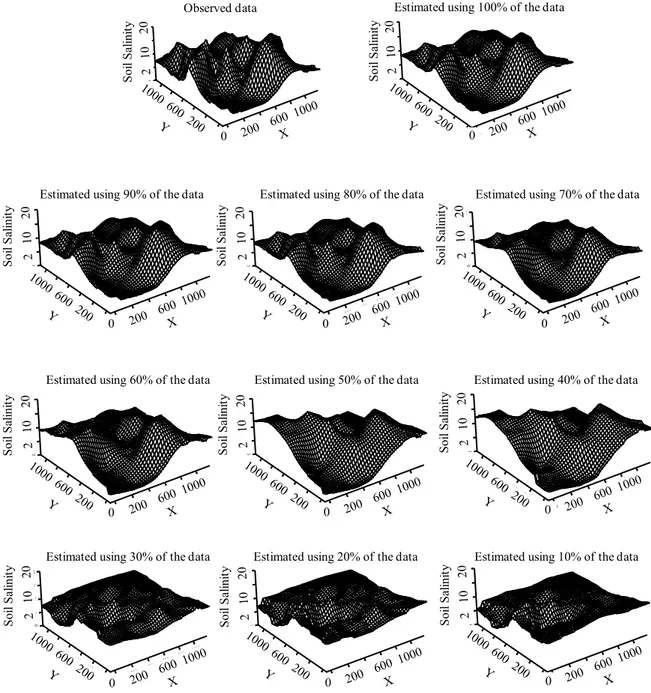
3.5. Example of Estimated Maps

Figures 5 shows an example of the observed and estimated three-dimensional dis-tributions of soil salinity for field US04 planted with alfalfa using the LANDSAT 5 im-age. Seventy-one sample points were collected in field US04 where the range of soil sa-linity was from 2.7-20.7 dS/m. For US04 the generated three-dimensional soil sasa-linity surfaces were acceptable for LANDSAT 5 image when using 60% or more of the data (43 points) and IKONOS image when using 50% or more of the data (36 points). Therefore, the variability of soil salinity in a given field plays a significant role in de-ciding the number of data points that need to be collected to adequately capture the structure of the distribution.

3.6. Model Validation

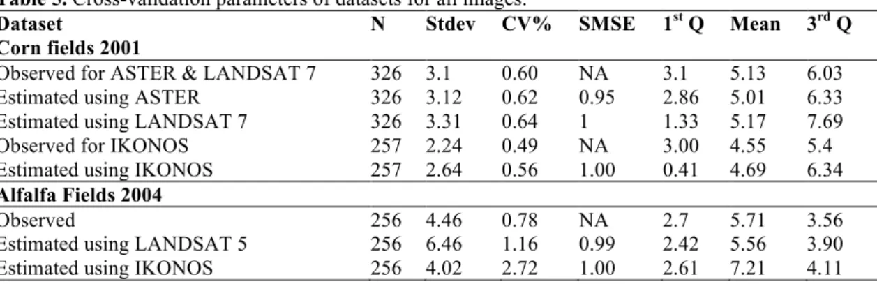
Table 5 shows the cross validation parameters of the datasets for all images with corn and alfalfa fields. For the 2001 corn field datasets, the ASTER and LANDSAT 7 images have a total of 326 sample points while the IKONOS image has a total of 257 sample points because field US10 was not covered by this image.

The standard deviation values of the observed and estimated data are very close for all datasets. The values of the coefficient of variation are 1.0 or less for all datasets, which means that the distributions of the datasets are considered to have low variance. The values of the SMSE for all datasets are 1.0 or less. The values of the first quartile and third quartile (1st Q and 3rd Q) of the observed and estimated data are close to each other.

(12)

Table 5. Cross-validation parameters of datasets for all images.

Dataset N Stdev CV% SMSE 1st_{Q Mean 3}rd_Q

Corn fields 2001

Observed for ASTER & LANDSAT 7 326 3.1 0.60 NA 3.1 5.13 6.03

Estimated using ASTER 326 3.12 0.62 0.95 2.86 5.01 6.33

Estimated using LANDSAT 7 326 3.31 0.64 1 1.33 5.17 7.69

Observed for IKONOS 257 2.24 0.49 NA 3.00 4.55 5.4

Estimated using IKONOS 257 2.64 0.56 1.00 0.41 4.69 6.34

Alfalfa Fields 2004

Observed 256 4.46 0.78 NA 2.7 5.71 3.56

Estimated using LANDSAT 5 256 6.46 1.16 0.99 2.42 5.56 3.90

Estimated using IKONOS 256 4.02 2.72 1.00 2.61 7.21 4.11

The observed values of the mean compared to the estimated values of all datasets are very close to each other. For the 2004 alfalfa fields, all four fields were covered by the two images and the number of sample points was 256. In general, the values of stand-ard deviation and coefficient of variation (CV) are slightly higher than those for the corn fields. However, the values of the standardized mean square error (SMSE) are al-most the same as those for the corn fields.

4. Conclusions

This research has shown that integrating field data, GIS, remote sensing and spatial modeling techniques can map and assess soil salinity. However, any integration of field data, GIS, and remote sensing is considered weak unless suitable statistical measures are introduced. The model that satisfies the assumption and selection criteria and has no autocorrelation in the residuals is not considered the best unless the estimated values of soil salinity match up relatively well with the observed values. This study introduced a methodology to merge field data with remote sensing data in order to obtain accurate soil salinity maps while reducing the number of soil samples that need to be collected. If a kriging technique is to be used for interpolation, the variograms should be imple-mented. The variograms play an important role in deciding how the data are correlated. When using kriging the higher the correlation among the data the better the interpola-tion. In this study, every time the datasets were reduced (i.e., the maximum distance be-tween correlated points increased) the variograms were constructed and inspected. With the help of variograms, the datasets could be reduced significantly. In this study the variograms show good fit with 40% or more of the observed data in corn fields which means that the number of collected points can be reduced from 326 to 130. In alfalfa fields, the variograms show good fit with 40% or more of the observed data, which means that the number of collected points can be reduced from 256 to 102. The meth-odology presented in this study performed well in estimating soil salinity when some of the data was removed and estimated using the remaining data. The variability in the da-ta in a specific field is more imporda-tant than the size of the field and therefore it is strongly recommended that as the range of observed soil salinity increases the number of soil salinity samples should increase in order to capture the variability in the field. The methodology worked better on fields planted with corn than on fields planted with alfalfa. The IKONOS images gave the best results when compared with the other satel-lite images used in this study. The LANDSAT 5, LANDSAT 7 and ASTER images performed similarly to each other. The fine resolution of the IKONOS images plays an important role in capturing the variability but as mentioned before, the selection of a specific image is a matter of judgment between the price and the resolution.

(13)

0 200 400 600 800 1000 X 0 200 40₀ 60₀ 80₀ 10₀₀ Y 0 5 10 15 20 Z 0 200 400 600 800 1000 X 0 200 40₀ 60₀ 800 10₀₀ Y 0 5 10 15 20 Z 0 200 400 600 800 1000 X 0 20₀ 400 60₀ 80₀ 10₀₀ Y 0 5 10 15 20 Z 0 200 400 600 800 1000 X 0 20₀ 40₀ 60₀ 800 10₀₀ Y 0 5 10 15 20 Z 0 200 400 600 800 1000 X 0 200 40₀ 60₀ 800 1000 Y 0 5 10 15 20 Z 0 200 400 600 800 1000 X 0 20₀ 40₀ 60₀ 80₀ 10₀₀ Y 0 5 10 15 20 Z 0 200 400 600 800 1000 X 0 200 40₀ 600 80₀ 1000 Y 0 5 10 15 20 Z 0 200 400 600 800 1000 X 0 20₀ 400 600 800 10₀₀ Y 0 5 10 15 20 Z 0 200 400 600 800 1000 X 0 20₀ 400 60₀ 80₀ 10₀₀ Y 0 5 10 15 20 Z 0 200 400 600 800 1000 X 0 20₀ 40₀ 60₀ 80₀ 10₀₀ Y 0 5 10 15 20 Z 0 200 400 600 800 1000 X 0 20 0 400 60 0 80 0 1000 Y 0 5 10 15 20 Z Observed data

Estimated using 90% of the data Estimated using 80% of the data Estimated using 70% of the data

S oi l S al ini ty 0 S oi l S al ini ty 0

Estimated using 100% of the data

S oi l S al ini ty 0 S oi l S al ini ty 0 S oi l S al ini ty 0 S oi l S al ini ty 0 S oi l S al ini ty 0 S oi l S al ini ty 0 S oi l S al ini ty 0 S oi l S al ini ty 0 S oi l S al ini ty 0

Figure 5. Observed and estimated surfaces of soil salinity (dS/m) of field US04 planted with alfalfa from

the ASTER image using all the observed

5. References

Bonham, C. D., R. M. Reich, and K. K. Leader. 1995. Spatial cross-correlation of Bouteloua gracilis with site factors. Grassland Science 41:196-201.

Bouma, J. (1984). Soil variability and soil survey. In: Bouma, J., Nielsen, D. (Eds.), Soil spatial variabil-ity workshop, Las Vegas, pp. 130-149.

Carr, J. R., Bailey, R. E., and Deng, E. D. 1985. “Use of indicator variograms for an enhanced spatial analysis.” Math. Geol.,17(8), 797–811.

Chung, C. K., Chong, S. K., and Varsa, E.C (1995). "Sampling strategies for fertility on a Stoy silt loam soil." Commun. Soil Sci. Plant Anal., 26(5/6), 741-763.

Cliff, A. D., and Ord, J. K. (1981). Spatial processes, models and applications, Pion Ltd., London, 21-45 Coper, R. M., and J. D. Istok. 1988a. Geostatistics applied to groundwater contamination I:

(14)

Coper, R. M., and J. D. Istok. 1988b. Geostatistics applied to groundwater contamination I: Application.

Journal of Environmental Engineering: 144, 287.

Davis, B.M. and Borgman, L., 1982. A note on the asymptotic distribution of the sample variogram. Math. Geol., 14: 643-653.

Di, H. J., Trangmar, B. B., and Kemp, R. A. (1989). "Use of geostatistics in designing sampling strate-gies for soil survey." Soil Sci. Soc. Am. J.,53940, 1163-1167.

Douaik, A., Van Meirvenne, M., and Toth, T.(2004). “Spatio-temporal kriging of soil salinity rescaled from bulk soil electrical conductivity.” Quantitative Geology And Geostatistics, GeoEnv IV: 4th Eu-ropean Conf. on Geostatistics For Environmental Applications, X. Sanchez-Vila, J. Carrera, and J. Gomez-Hernandez, eds., Kluwer Academic, Dordrecht, The Netherlands, 13(8) 413–424.

Efron, B., and R. J. Tibshirani. 1993. An introduction to the bootstrap. Chapman and Hall: New York, New York.

Eldeiry, A.A. and L.A. Garcia. 2008a. Spatial modeling of soil salinity using remote sensing GIS, and field data. VDM Verlag.

Eldeiry, A.A. and L.A. Garcia. 2008b. Detecting soil salinity in alfalfa fields using spatial modeling and remote sensing. Soil Science Society of America Journal 72, no. 1 (Jan.-Feb.): 201-211.

Eldeiry, A.A. and L.A. Garcia. 2010. Comparison of ordinary kriging, regression kriging, and cokriging techniques to estimate soil salinity using LANDSAT images. ASCE Journal of Irrigation and Drain-age Engineering 136:355.

ERDAS Imagine. 2006. ERDAS Inc., Leica Geosystems, 2801 Buford Highway, Atlanta, GA 30329. Gates, T. K., J. P. Burkhalter, J. W. Labadie, J. C. Valliant, and I. Broner. 2002. Monitoring and

model-ing flow and salt transport in a salinity-threatened irrigated valley. Journal of Water Resources

Planning and Management 128, no. 2:87-99.

Geisser, S. 1975. The predictive sample reuse method with applications. The Journal of American

Statis-tical Association 70:320-328.

Hevesi, J.A., J. D. Istok and A. L. Flint. 1992. Precipitation estimation in mountainous terrain using mul-tivariate geostatistics part I: structural analysis. Journal of Applied Meteorology 31, no. 7:661–676. Hill, M. J., and Donald, G. E. (2003). Estimating spatio-temporal patterns of agricultural productivity in

fragmented landscapes using AVHRR NDVI time series. Remote Sensing of Environment 84, no. 3:367-384.

Hillel, D. (2000). Salinity management for sustainable irrigation: Integrating science, environment, and economics, The World Bank, Wash-ington, D.C.

Istok, J. D. and R. M. Cooper. 1988. Geostatistics applied to groundwater pollution, III: Global esti-mates. Journal of Environmental Engineering :114, 915.

Journel, A. G., and Ch. J. Huijbregts. 1978. Mining geostatistics. Academic Press (London):600. McBratney, A. B., and Webster, R. (1983). "How many observations are need for regional estimation of

soil properties?" Soil Sci., 135(3), 177-183.

McBratney, A. B., I. O. A. Odeh, T. F. A. Bishop, M. S. Dunbar, and T. M. Shatar. 2000. An overview of pedometric techniques for use in soil survey. Geoderma 97:293-327, doi:10.1016/S0016-7061(00)00043-4.

Moran, P. A. P. 1948. The interpretation of statistical maps, Royal Statistics Society B, no. 10:243-351. Myers, D.E., 1991. On variogram estimation. In: E. Dudewicz et al. (Editors), The Frontiers of Statistical

Scientific Theory and Industrial Applications. Proc. of OCOSCO-I, Vol. II. American Sciences Press, pp. 261-28 I.

Nielsen, D. R., P. M. Tillotson, and S. R. Viera. 1983. Analyzing field measured soil-water properties.

Agriculture Water Management 6:93-109.

Phillips, J. D. 1985. Measuring complexity of environmental gradients. Vegetatio 64:95-102.

Pozdnyakova, L. and Zhang, R. 1999. Geostatistical analyses of soil salinity in a large field. Precision

Agriculture 1:153-165.

Reich, R. M., R. L. Czaplewaki, and W. A. Bechthold. 1994. Spatial cross-correlation of undisturbed natural shortleaf pine stands in northern Georgia. Journal of Environmental and Ecological Statistics 1:201-217.

Robertson, G. P. 1987. Geostatistics in ecology: Interpolating with known variance. Ecology 68, no. 3 (Jun.):744-748

Schloeder, C. A., N. E. Zimmermann, and M. J. Jacobs. 2001 Comparison of methods for interpolating soil properties using limited data. Soil Science Society of America Journal 65:470–479.

Stone, M. 1974 Cross-validation choice and assessment of statistical predictions. Journal of the Royal

Statistical Society B 36:111-133.

Utset, A., M. E. Ruiz, J. Herrera, and D. Ponce de Leon. 1998. A geostatistical method for soil salinity sample site spacing. Geoderma 86:143-151.

(15)

Warrick, A. W., D. E. Myers, and D. R. Nielsen. 1986. Geostatistical methods applied to soil science.

Soil Science Society of America Journal Agronomy Monograph, no. 9.

Watson, P.K., and S.S. Teelucksingh. 2002. A practical introduction to econometric methods: Classical and modern. Univ. of West Indies Press, Kingston, Jamaica.

Webster, R., and M. A. Oliver. 1990. Statistical methods in soil and land survey, spatial information sys-tems. Oxford University Press: Oxford,UK

White, R. E. 1997. Principles and practice of soil science: The soil as a natural resource. Blackwell Sci-ence Ltd: Oxford.

Wiegand, C. L., J. D. Rhoades, D. E. Escobar, and J. H. Everitt. 1994. Photographic and videographic observations for determining and mapping the response of cotton to soil salinity. Reomte Sensing of

Environment 49:212-223.

Wilding, L. (1984). Spatial variability. Its documentation, accomodation and implication to soil survey. In: Bouma, J., Nielsen, D. (Eds.), Soil variability workshop, Las Vegas, pp. 163-171.

Yamaguchi, Y., A. B. Kahle, H. Tsu, T. Kawakami, and M. Pniel. 1998. Overview of advanced space-borne thermal emission and reflection radiometer (ASTER). IEEE Transactions on Geoscience and