THESIS
ACCOUNTING FOR WELL CAPACITY IN THE ECONOMIC DECISION MAKING OF GROUNDWATER USERS
Submitted by Samuel Collie
Department of Agricultural and Resource Economics
In partial fulfillment of the requirements For the Degree of Master of Science
Colorado State University Fort Collins, Colorado
Summer 2015
Master’s Committee:
Advisor: Jordan Suter Dale Manning
Copyright by Samuel Collie 2015 All Rights Reserved
ABSTRACT
ACCOUNTING FOR WELL CAPACITY IN THE ECONOMIC DECISION MAKING OF GROUNDWATER USERS
Water conflicts unfolding around the world present the need for accurate economic models of groundwater use which couple traditional producer theory with hydrological science. We present a static optimization problem of individual producer rents, given groundwater as a variable input to production. In a break with previous literature, the model allows for the possibility of binding constraints on well capacity, which occur due to the finite lateral speed at which water moves underground. The theoretical model predicts that binding well yield
constraints imply producers extract as much water as possible to maximize profit. Therefore, if producers are constrained, regions with more available water should consume more of it. We test this hypothesis empirically by modelling the effect of well yields on crop cover and water usage data. Our empirical results find that areas with higher than average well capacities tend to plant a more water intensive mix of crops, and use more groundwater. This straightforward result comes in contrast to previous economic models of groundwater use, which have assumed an interior solution to the irrigators’ profit maximization problem. Well capacity also affects how farmers respond to seasonal weather variation. Farms with high well capacity react sharply to seasonal precipitation, whereas low capacity farms show less adjustment. This research provides
important inroads to understanding what drives irrigators’ behavior on the High Plains; a crucial step towards conserving this resource.
TABLE OF CONTENTS
ABSTRACT ... ii
I. INTRODUCTION ...1
II. LITURATURE REVIEW ...5
III. HYDROLOGY CONCEPTS ...8
IV. THEORETICAL MODEL...11
V. EMPIRICAL APPLICATION ...18
VI. CONCLUSION...33
VII. REFERENCE LIST ...38
A1. SATELLITE DATA AND GIS PROCEDURES ...41
I. INTRODUCTION
Groundwater depletion in the High Plains aquifer raises concerns that existing institutions which govern groundwater usage do not maximize the economic potential of the resource.
Groundwater access on the High Plains is governed by incomplete property rights. Multiple externalities persist in the usage of groundwater resources (Provencher & Burt 1993), meaning the private incentives of individual profit-maximizing firms do not align with social objectives. Economic theory suggests that the uncoordinated actions of individuals sharing a common pool resource, such as the groundwater in an aquifer, will lead to an inefficient outcome known as the ‘tragedy of the commons’ (Hardin 1968). Individuals who have access to a finite common-pool resource, but do not own it, have less incentive to conserve the resource for future use.
An extensive literature has considered this divergence between individually rational and socially optimal groundwater use (Koundouri 2004). Many of these studies compare a myopic strategy, in which an indivual maximizes annual profits and ignores future stock-dependent costs, to a socially optimal outcome in which net benefits achieve a dynamic maximum. More recently, the groundwater management literature has considered which type of strategy better depicts groundwater users’ behavior in the context of more realistic models of an aquifers’ response to pumping. A lab experiment by Suter et al. (2012) showed that the answer depends on the spatial nature of groundwater use and the aquifers’ characteristics. In settings where
geological factors result in more complete ownership of groundwater, usage more closely resembles a privately optimal dynamic strategy. In settings where groundwater is more shared and the costs of use are spread evenly across users, individuals’ actions will more closely resemble a myopic strategy.
The distinction between the two strategies is important because ultimately it will dictate the size of the welfare loss associated with open-access. At one extreme is the tragedy of the commons, and at the other is complete private ownership and dynamically optimal resource extraction. While considerable research has compared the welfare implications between each strategy, less research has attempted to describe which strategy actually depicts groundwater usage in real-world settings. A notable exception is a study of groundwater users in Kansas (Pfieffer & Lin 2012), which finds that groundwater-users in fact consider the negative impact of their pumping on future groundwater stocks. Instead of maximizing total annual profits,
producers are said to dynamically balance the benefits and costs of groundwater extraction over time. To support this hypothesis, this literature points out that groundwater users in Kansas rarely consume as much groundwater as they are legally entitled to; despite institutions governing groundwater which practically encourage them to do so. As further evidence, these studies show that certain aquifer characteristics are in fact correlated with observed groundwater extraction patterns.
In this paper, we propose an alternative explanation for the correlation between aquifer characteristics and groundwater use. We extend the static optimization problem of the short-sighted producer to allow for instantaneous constraints on groundwater supplies. Well capacity constraints are physical limitations on the amount of water available to produce from a well, due to the very gradual nature of water movement underground. The model predicts that when well capacity constraints bind, producers maximize profit by extracting as much water as possible. This simple result reveals a connection between observed pumping quantities and aquifer characteristics, regardless of whether or not producers optimize dynamically.
With this in mind, we revisit the Kansas water use data, and the variables which have previously been associated with a dynamic extraction strategy. Over a study period of 2006 to 2013, areas with higher than average well capacities saw more area planted with water intensive crops, and applied more irrigation per acre planted. These results are in line with previous econometric studies that find a positive correlation between the size of groundwater stocks and extraction quantities (Pfeiffer & Lin 2012, 2014b). However, these studies attribute the
relationship to a dynamic extraction pattern exercised by farmers, reasoning that farmers with smaller groundwater stocks consume less, knowing their future supplies are limited.
We present evidence that well capacity constraints play a role in the irrigation decisions of farmers. We argue that well capacity constraints present a second possible explanation for the positive correlation between groundwater stocks and water usage. To strengthen our argument, we analyze groundwater users’ responsiveness to seasonal precipitation. If well capacity does restrict water usage, then irrigators with higher well capacity should have a greater ability to react to precipitation. Capacity constraints impose an upper limit on the amount of groundwater available to extract during one growing season. Therefore during drought years, farms with low well capacity might not be able to meet crop water requirements, and will appear unresponsive to precipitation. Matching farmers’ well-sites to spatially referenced precipitation data allows us to test this reasoning. Farms with high well capacities show the sharpest adjustment to seasonal precipitation, whereas farms with low capacity make less of an adjustment. This result strengthens the argument that capacity constraints influence water use decisions on the High Plains.
As groundwater levels across the High Plains continue to fall, well capacity constraints will be an increasing reality for agricultural producers on the High Plains (Schneekloth 2015).
This thesis addresses the role that capacity constraints play in producer decisions and provides supporting empirical evidence that highlights the importance of capacity constraints on the behavior of groundwater users.
II. LITURATURE REVIEW
This research adds to a growing body of literature which couples economic producer theory with spatially complex aquifer characteristics. In the past, economists studied
groundwater use in the context of a simplistic single cell, or ‘bathtub’ aquifer. Resource users were said to draw groundwater from an underground bathtub, in which the water level would decline uniformly as the result of any users’ pumping. The seminal paper utilized dynamic programming methods to show that welfare gains from optimal control were negligible when compared to a baseline competitive pumping scenario (Gisser & Sanchez 1980). The so-called ‘Gisser-Sanchez Paradox’ has since been tested, and proven surprisingly resilient, to more robust sets of assumptions (Koundouri 2004). The Gisser-Sanchez model and its contemporaries follow the same basic procedure, in which discounted future net benefits of an optimal control
extraction path are compared to competitive pumping scenarios. In the optimal control, pumping quantities are chosen to maximize the present value of social benefits. This depicts the pumping choice of a benevolent social planner, or that of an irrigator if they had complete ownership of the resource. In the competitive model, pumpers act myopically, and equate the private marginal benefits and costs of extraction.
Early research may have found little potential for welfare improving groundwater management, but it is unclear how well it depicts the pumping decision of actual irrigators who draw from aquifers with complex spatial characteristics. These papers utilize a ‘bathtub’ characterization of groundwater hydraulics, in which the drawdown caused by pumping is uniform across space. In reality, groundwater pumping forms a localized aquifer drawdown known as a cone of depression (Weight & Sonderegger 2001). This phenomenon, coupled with the fact that groundwater movement can be extremely gradual, suggests that groundwater can be
more of a private, rather than public resource. This topic was the focus of a study by Suter et al. (2012), conducted in the controlled setting of a laboratory economics experiment. The study found that levels of resource use were higher when the costs of use were more shared amongst users.
In the past decade, there has been a push among economists to extend the ‘bath-tub’ aquifer characterization, to more realistic, spatially explicit settings. In a series of papers by Brozović et al. (2006, 2010), the basic model of optimal control versus competitive pumping was extended to incorporate hydrologic equations of lateral groundwater flow. In contrast to the bathtub characterization, these papers calculated the effect of pumping on aquifer drawdown across space, using hydrology’s Theis equation (Theis 1935). Guilfoos et al. (2013)
parameterized a multi-cell aquifer model using data from Kern County, California, and found that gains from management were significantly higher in the spatially explicit setting, versus the bath-tub model.
A very recent branch of literature considers finite speeds of groundwater flows in a different light. Instead of considering how aquifer properties influence potential gains from groundwater management, this branch of literature considers how groundwater flows influence extraction decisions at the producer level. Foster et al. (2014) simulate the effect of hydrologic constraints on irrigators’ decision making. In their model, irrigators react to climatic variation based on a previously chosen soil moisture target. A follow-up study (Foster et al. 2015),
provides a comprehensive analysis of well capacities using observational data. The study utilizes well completion records from Nebraska’s portion of the Republican River Basin, to compare well capacities to the size of irrigated acreage, and the saturated thickness of the underlying aquifer. The study finds that agricultural productivity exhibits a non-linear relationship to saturated
thickness, and that well-capacity has a stronger influence on producers’ decisions than depth to water (Foster et al. 2015).
Well capacity constraints have been shown to have substantial economic impacts outside the realm of groundwater resources. A working paper from the National Bureau of Economic Research highlights the divergence between observed extraction patterns of crude oil, and those predicted by economic theory (Anderson et al. 2014). Historically, oil extraction from existing wells has not responded to changing price incentives, in the way that the Hotelling model of non-renewable resource extraction would suggest. Anderson et al. propose that well capacity
constraints can explain the divergence between theory and observed oil extraction. Like
groundwater wells, the maximum rate at which oil can be extracted from a well is determined by biophysical factors. As a consequence, oil producers have a limited ability to adjust production quantities in the short-run. Anderson’s empirical results show that well capacity constraints limit producers’ response to price incentives in the short-run; although in the long-run, oil producers can respond by drilling more wells.
III. HYDROLOGY CONCEPTS
The fundamental objective of this research is to point out that every groundwater well has a finite capacity, and to illustrate how a well’s capacity can influence groundwater users’
economic decisions. Up to this point, the term ‘well capacity’ has been used to loosely describe the maximum quantity of groundwater that can be produced from a well, in a given period of time. In the following analysis, reported rates of pumping are used as a proxy for overall well capacity, which makes it critical to establish the connection between these two related terms. A pumping rate is a volume of fluid passing a point per unit time. Pumping capacity is defined as the maximum pumping rate a well can sustain for an extended period of time. The connection between observed pumping rates, and a well’s overall capacity to produce water, might not be immediately intuitive. For that reason, the following section provides a brief primer on the mechanics of irrigation systems, as well as the hydrologic factors which dictate well capacity.
An aquifer is a geologic formation comprised of porous mediums, such as sand or
fractured rock. An underlying dense layer of clay or bedrock prevents water from seeping deeper into the earth. The porous nature of an aquifer is critical to its overall quality. Hydrologists use the term transmissivity to describe rates of groundwater flow within an aquifer (Todd & Mays 2005). Transmissivity can be broken down into two components, hydraulic conductivity and saturated thickness. Hydraulic conductivity is the potential water velocity through a given aquifer layer. However, only saturated layers can contribute to groundwater flow. Therefore transmissivity is equal to the aquifers’ hydraulic conductivity integrated across its saturated thickness. Transmissivity plays a critical role in determining well capacity, as it influences the potential for groundwater movement towards the well.
When groundwater is drawn from a well, a cone of depression is formed in the water table around the well site. The size of the cone of depression which results from pumping groundwater is influenced by the aquifers’ conductivity. Higher conductivity corresponds to a shallower cone of depression, while low conductivity results in steep draw down (Weight & Sonderegger 2001). Thus, for a given level of saturated thickness, areas with high conductivity can sustain greater pumping volumes, without the cone of depression intruding the well screen.
In practice, well capacity can be calculated with a well test. A well test involves running a well for an extended period, and measuring the resulting draw down inside the well. The well test allows engineers to parametrize analytic models pioneered by Theis (1935), which are used to quantify an aquifer’s response to pumping. These formulas enable engineers to calculate the aquifer transmissivity surrounding the well (Weight & Sonderegger 2001).
The hydrologic factors which influence pumping capacity are well known, yet few existing studies have systematically analyzed well capacity across aquifer properties. Well tests are typically conducted by and for private individuals, meaning data collected across multiple test sites are not readily available. A notable exception utilized records from Nebraska’s portion of the Republican River Basin, and found that well capacity had a strong influence on water use decisions (Foster et al. 2015). The only other known study was conducted by the Kansas
Geological Survey, which relied on numerical methods to estimate the minimum saturated thickness required to sustain a given pumping rate for a range of aquifer parameters (Hecox et al. 2002).
Given that so few sources of true well capacity data exist, the water use data from Kansas has some key advantages. Unlike well tests, which are usually conducted when a new well is installed, the Kansas data reveals how pumping capacities have evolved over time. The Kansas
data also includes annual groundwater extraction quantities, which provides the means to analyze how pumping capacity influences groundwater users’ decision making. The drawback to the Kansas data is that farmers’ pumping rates are reported, not their true maximum well capacity as measured by a well test.
Nevertheless, reported pumping rates are a useful proxy for well capacity. Farmers with limited well capacity face incentives to set pumping rates as high as they can. At the peak of summer, daily crop water requirements will outstrip supply, meaning farmers pump as fast as possible, in order to minimize yield losses due to water stress. On the other hand, farmers also face incentives not to be overly optimistic about their wells’ capacities. Irrigation systems are left continuously running during parts of the growing season, with center pivots set to make a
complete revolution once every four to eight days. To ensure an even coverage of irrigation, this management practice requires that a well be set to a sustainable capacity. Reported pumping rates therefore represent a lower bound for well capacity, since the well must be able to produce at least as much water as was reported.
IV. THEORETICAL MODEL
The goal of this section is to explore how potential well capacity constraints affect agricultural producers’ decision making. The theoretical model describes the problem of a representative farm, seeking to maximize annual profits. The farm must choose which crops to grow, and how much land and water to allocate to each crop grown. Both land and water choices are subject to physical constraints which may limit their use. The model’s simplest possible case shows how aquifer properties can influence water use decisions. The model predicts a high degree of correlation between aquifer properties and water usage, in the context of a static optimization problem. Thus, the theoretical model provides a linkage between aquifer characteristics and groundwater use, which is not necessarily due to a dynamic extraction strategy.
In the model, two distinct decision stages describe the profit maximization problem of an individual farmer. In the first stage, the farmer must decide how to divide their land between crops, given uncertainty about the weather. In the second stage, the farmer chooses how much to irrigate each crop, once the weather is known. A two-stage stochastic dynamic program is used to solve both stages. In the simplest case, there are two possible crops, and two potential weather outcomes. For example, the farmer might choose between planting a more or less water intensive crop (e.g., corn or wheat), and may experience a rainy or dry growing season.
Expected profits in the first stage are the sum of profits associated with each weather outcome, multiplied by the probability ε, or (1- ε), of experiencing a rainy or dry growing season, respectively. The farmer chooses the number of acres to plant to wheat and corn, aw, and ac,
subject to a constraint on the overall field size 𝐴𝐴̅.
Stage 1:
Maxaw,ac: E[π] = ε ∗ πr(aw, ac| w, 𝐏𝐏, 𝛙𝛙) + (1 − ε) ∗ πd(aw, ac| 𝑤𝑤, 𝐏𝐏, 𝛙𝛙) (1) 𝑆𝑆𝑆𝑆𝑆𝑆𝑆𝑆𝑆𝑆𝑆𝑆𝑆𝑆 𝑆𝑆𝑡𝑡: 𝑎𝑎𝑤𝑤+ 𝑎𝑎𝑐𝑐 ≤ 𝐴𝐴̅
The profit earned under the rainy and dry outcomes are denoted 𝜋𝜋𝑟𝑟 and 𝜋𝜋𝑑𝑑. Profits depend on the quantity of irrigation supplied, denoted w, a vector of input and output prices P, and a vector of farm specific attributes 𝝍𝝍. Farm-specific attributes include soil quality, depth to groundwater, average climate conditions, and the overall size of the farm.
In the second stage, the farmer chooses the quantity of irrigation to apply, conditional on the number of acres planted, and the weather outcome. Revenues depend on the rainfall event, k ϵ {dry, rainy}, as well as prices and the site-specific variables. In stage 2, the total quantity of irrigation applied, w, is equal to the well pumping capacity, Θ, multiplied by the amount of time that the well was operated, ℎ. These components reflect the two ways irrigation quantities can be adjusted. Two constraints limit the choice of w in stage 2. The amount of time spent irrigating cannot exceed the season length, 𝐻𝐻�. Legal restrictions on permitted volume may also constrain the amount of irrigation applied, so that w ≤ 𝑊𝑊� .
Stage 2:
𝑀𝑀𝑎𝑎𝑀𝑀𝑤𝑤: 𝜋𝜋 = 𝜋𝜋𝑘𝑘(𝑤𝑤 | 𝑎𝑎𝑤𝑤, 𝑎𝑎𝑐𝑐, 𝑷𝑷, 𝝍𝝍) (2) 𝑆𝑆𝑆𝑆𝑆𝑆𝑆𝑆𝑆𝑆𝑆𝑆𝑆𝑆 𝑆𝑆𝑡𝑡: 𝑤𝑤 𝛩𝛩⁄ ≤ 𝐻𝐻�, and w ≤ W� .
Where: k ϵ {dry, rainy}, and w = ℎ ∗ Θ
The two-stage dynamic program can be solved recursively, starting with stage 2. Stage two is solved for each distinct weather outcome, k ϵ {dry, rainy}. The Lagrangian for the stage 2 decision follows:
𝑀𝑀𝑎𝑎𝑀𝑀𝑤𝑤: 𝐿𝐿 = 𝜋𝜋𝑘𝑘(𝑤𝑤 | 𝑎𝑎𝑤𝑤, 𝑎𝑎𝑐𝑐, 𝑷𝑷, 𝝍𝝍) + 𝜆𝜆1(𝐻𝐻� ∗ 𝛩𝛩 − 𝑤𝑤) + 𝜆𝜆2(𝑊𝑊� − 𝑤𝑤)
First Order Conditions: 𝜕𝜕L 𝜕𝜕𝑤𝑤 = 𝜕𝜕𝜋𝜋𝑘𝑘(.) 𝜕𝜕w − 𝜆𝜆1− 𝜆𝜆2 ≤ 0 c.s. 𝑤𝑤 ≥ 0 𝜕𝜕L 𝜕𝜕𝜆𝜆1= 𝐻𝐻� ∗ 𝛩𝛩 − 𝑤𝑤 ≥ 0 c.s. 𝜆𝜆1 ≥ 0 𝜕𝜕L 𝜕𝜕𝜆𝜆2= 𝑊𝑊� − 𝑤𝑤 ≥ 0 c.s. 𝜆𝜆2 ≥ 0
The first order conditions can be solved for each possible weather event. The solutions implied by the first order conditions are: 𝑤𝑤𝑟𝑟∗(𝑎𝑎𝑤𝑤, 𝑎𝑎𝑐𝑐, 𝑷𝑷, 𝝍𝝍, 𝛩𝛩, 𝐻𝐻�, 𝑊𝑊� ) and
𝑤𝑤𝑑𝑑∗(𝑎𝑎
𝑤𝑤, 𝑎𝑎𝑐𝑐, 𝑷𝑷, 𝝍𝝍, 𝛩𝛩, 𝐻𝐻�, 𝑊𝑊� ). Profit maximizing irrigation quantities are a function of the acreage decision, prices, farm specific attributes, pumping capacity, growing season length, and possible legal constraints. These solutions are plugged into the stage 1 decision, to solve for the profit maximizing acreage allocation.
𝑀𝑀𝑎𝑎𝑀𝑀𝑎𝑎𝑤𝑤,𝑎𝑎𝑐𝑐: 𝐿𝐿 = 𝜀𝜀 ∗ 𝜋𝜋𝑟𝑟(𝑎𝑎𝑤𝑤, 𝑎𝑎𝑐𝑐|𝑤𝑤𝑟𝑟∗(. ), 𝑷𝑷, 𝝍𝝍) + (1 − 𝜀𝜀) ∗ 𝜋𝜋𝑑𝑑(𝑎𝑎𝑤𝑤, 𝑎𝑎𝑐𝑐|𝑤𝑤𝑑𝑑∗(. ), 𝑷𝑷, 𝝍𝝍) + 𝜆𝜆(𝐴𝐴̅ − 𝑎𝑎𝑤𝑤− 𝑎𝑎𝑐𝑐)
First Order Conditions:
𝜕𝜕L 𝜕𝜕𝑎𝑎𝑤𝑤 = 𝜀𝜀 ∗ � 𝜕𝜕𝜋𝜋𝑟𝑟(.) 𝜕𝜕𝑎𝑎𝑤𝑤 + 𝜕𝜕𝜋𝜋𝑟𝑟(.) 𝜕𝜕𝑤𝑤𝑟𝑟∗(.) 𝜕𝜕𝑤𝑤𝑟𝑟∗(.) 𝜕𝜕𝑎𝑎𝑤𝑤 � + (1 − 𝜀𝜀) ∗ � 𝜕𝜕𝜋𝜋𝑑𝑑(.) 𝜕𝜕𝑎𝑎𝑤𝑤 + 𝜕𝜕𝜋𝜋𝑑𝑑(.) 𝜕𝜕𝑤𝑤𝑑𝑑∗(.) 𝜕𝜕𝑤𝑤𝑑𝑑∗(.) 𝜕𝜕𝑎𝑎𝑤𝑤 � − 𝜆𝜆 ≤ 0 c.s. 𝑎𝑎𝑤𝑤 ≥ 0 𝜕𝜕L 𝜕𝜕𝑎𝑎𝑐𝑐= 𝜀𝜀 ∗ � 𝜕𝜕𝜋𝜋𝑟𝑟(.) 𝜕𝜕𝑎𝑎𝑐𝑐 + 𝜕𝜕𝜋𝜋𝑟𝑟(.) 𝜕𝜕𝑤𝑤𝑟𝑟∗(.) 𝜕𝜕𝑤𝑤𝑟𝑟∗(.) 𝜕𝜕𝑎𝑎𝑐𝑐 � + (1 − 𝜀𝜀) ∗ � 𝜕𝜕𝜋𝜋𝑑𝑑(.) 𝜕𝜕𝑎𝑎𝑐𝑐 + 𝜕𝜕𝜋𝜋𝑑𝑑(.) 𝜕𝜕𝑤𝑤𝑑𝑑∗(.) 𝜕𝜕𝑤𝑤𝑑𝑑∗(.) 𝜕𝜕𝑎𝑎𝑐𝑐 � − 𝜆𝜆 ≤ 0 c.s. 𝑎𝑎𝑐𝑐 ≥ 0 𝜕𝜕L 𝜕𝜕𝜆𝜆 = 𝐴𝐴̅ − 𝑎𝑎𝑤𝑤 − 𝑎𝑎𝑐𝑐 ≥ 0 c.s. 𝜆𝜆 ≥ 0
The solutions for the acreage allocation are 𝑎𝑎𝑤𝑤∗(𝜀𝜀, 𝑷𝑷, 𝝍𝝍, 𝛩𝛩, 𝐻𝐻�, 𝑊𝑊� ) and
𝑎𝑎𝑐𝑐∗(𝜀𝜀, 𝑷𝑷, 𝝍𝝍, 𝛩𝛩, 𝐻𝐻�, 𝑊𝑊� ). Critically, the area allocated to each crop, and the number of hours of irrigating, both depend on 𝛩𝛩, the well’s pumping capacity. The capacity constraint reveals a
connection between aquifer characteristics and pumping behavior, even when producers do not optimize dynamically.
In an aggregate view, there likely exists a mix of constrained and unconstrained water users. This can raise problems when analyzing groundwater data, which generally does not reveal if a producer is capacity constrained. Nevertheless, statistics drawn across the entire population have consistently found that groundwater users exhibit very low price-elasticity of water demand (Scheierling et al. 2006). Extremely low elasticity of demand estimates could be due to capacity constrained producers’ inability to respond to changing marginal incentives.
Figure 1 illustrates the effect of well capacity constraints on an individual farmers’
groundwater demand. The figure depicts two possibilities, in which a farmer is either constrained or unconstrained by well capacity. For the unconstrained producer, water use is determined by the intersection of the marginal cost and benefit curves. Two marginal cost curves are shown, signifying that an upward shift in marginal costs will result in less water use by the
unconstrained producer. Water consumption by the unconstrained producer shifts from 𝑤𝑤𝑈𝑈𝑈𝑈1 to 𝑤𝑤𝑈𝑈𝑈𝑈2 . For the capacity constrained farmer, the shift in marginal costs does not affect the amount of water used. Total water consumption is equal to 𝑤𝑤𝑈𝑈1,2 in both cases. The illustration shows that a water constrained producer will appear very unresponsive to shifts in the marginal incentives of water use.
Having considered the theoretical model’s predictions for optimal water use, we now turn to the irrigator’s optimal land use decision. The specific question addressed is how capacity constraints inform a farms’ acreage allocation. The water constraint could be caused by multiple factors, including well capacity or legal restrictions. Water constrained farmers have two
choices: they may either reduce the amount of water used per-acre, or plant less acres of water
intensive crops. On the High Plains, farmers with low capacity wells have been found in previous research to overplant corn and subject themselves to potentially large yield losses, in the hopes that favorable weather will induce an economic windfall (Schneekloth 2012, 2015). When the weather does not cooperate, crop insurance serves as an economic backstop.
Figure 1. Profit maximizing water use when supply is constrained and unconstrained.
The two stage maximization problem presented earlier can be used to explain this behavior. In the two crop example, the first order conditions are such that the expected net marginal gain of planting either wheat or corn is equal. Once the well capacity constraint is reached, there will be diminishing returns to planting the water intensive crop. This occurs because the crop receives less irrigation than the full requirement, which will impact its yield.
D
olla
rs
Water
� 𝐻𝐻*𝛩𝛩 𝑤𝑤𝑈𝑈𝑈𝑈1 𝑤𝑤𝑈𝑈1,2 MB 𝑤𝑤𝑈𝑈𝑈𝑈2 MC1 MC2 15Despite losses in crop yields per acre, ultimately the marginal benefit of the alternate land use determines the optimal field size. On the High Plains, growing irrigated corn has been lucrative, making it optimal to accept yield losses in comparison to growing less water intensive crops. The problem with this strategy is that it results in inefficient water usage. Low capacity farms adopt strategies like pre-watering fields before planting, and running irrigation during rain events, to try to keep up with the season’s anticipated irrigation deficit. Often, these farms cannot supply enough water in the heat of summer when corn growth is at its most sensitive stages.
Corn evapotranspiration data from Kansas State’s Northwest Research Station was used to generate Figure 2. On average, daily corn irrigation requirements peak around the end of July. The figure shows the daily water requirements for a typically sized, 120 acre center pivot. If no precipitation or soil moisture is available for crop use, an irrigation system with 90% efficiency would need to pump over one million gallons of water per day at the peak of summer. Left continuously running, the well would have to pump at 754 gallons per minute in order to meet the full crop-water requirement.
Figure 2: Daily Corn ET Requirement for a 120 Acre Pivot, Source: Kansas State University Northwest Area Extension, Colby Kansas, 2004-2014
V. EMPIRICAL APPLICATION
In this section, the implications of well capacity constraints are examined using agricultural groundwater use data from Kansas. Since 1990, Kansas has mandated that
groundwater wells install meters and report total annual withdrawals. These records are part of the Water Rights Information System (WRIS) dataset and are publically available online.
Numerous economic studies have made use of Kansas’ high quality groundwater data, including Hendricks and Peterson (2012), and Pfeiffer and Lin (2012, 2013, 2014a, 2014b). The data is comprised of the spatial locations of each well-site, as well as corresponding annual water use records from 1990-2013. Each observation includes an identification number of the person who filled out the report. For some observations, the data includes the well’s pumping rate, as well as the total accumulated amount of water use.
An additional set of records contains the spatial locations of land tracts authorized for use with irrigation, and a list of each water right that is legally authorized to apply water on that acreage. The tracts of land in the data are ‘quarter-quarter’ 40 acre sections, categorized by the Public Land Survey System (PLSS). A typical center pivot irrigation system comprises four of these sections, covering a rectangular area of 160 acres. Linking these PLSS sections back to the annually reported water use data allows us to collect data on farmers’ cropping decisions at an unprecedented level of spatial clarity.
Previous studies using Kansas’s groundwater use data have relied on crop acreage numbers self-reported by farmers in the WIMAS dataset. This crop data has severe limitations, as described in Pfieffer and Lin (2014a), “The WIMAS does not report yields, and in many cases, the data containing the crop planted on the field cannot be used to calculate the acreage planted to each crop. The data reporter is asked to code the crops that were planted in a field, but
not the proportion of the field planted to each crop. For example, a field planted in half corn and half wheat would look the same in the data as a field planted in corn with wheat planted in the center pivot corners. Ideally, we would like to study the relationship between the use of more efficient irrigation and crop acreage decisions. However, this would involve potentially inaccurate assumptions about the proportion of crops planted to each multi-cropped field.” Hendricks and Peterson (2012) encountered the same problem, stating, “The most common irrigated crops grown in Kansas are corn, soybeans, alfalfa, wheat, and sorghum. ‘Other’ crops include sunflowers, barley, oats, rye, and dry beans. About 32% of the observations reported that the field was split between crops. Unfortunately, the number of acres planted to each crop in these situations was not reported, nor was the water applied to each crop.”
We overcome this obstacle by gathering additional satellite land cover data at the PLSS section level, sourced from the United States Department of Agriculture’s National Statistics Service. In the ambiguous situations when farmers split fields between multiple crops, satellite land cover data allows us to discern exactly how many acres of each crop were grown. Several papers have used this data in the context of groundwater pollution, including Fitzgerald and Zimmerman (2013), and Hendricks et al. (2014). The Cropland data layers are raster images of the United States, in which each pixel of the image corresponds to a specific crop.
The raster files have a 30 by 30 meter resolution; a land area of less than a quarter of an acre. The crop cover data for Kansas are available for the years 2006-2013, in which an eight year panel of water and land use data are available. A crucial step in linking these two sources of data was using individual farmer-year combinations as the unit of analysis. The water use data is recorded for each well site, but often multiple wells are authorized to irrigate the same tract of land. Grouping observations at the farmer level greatly improved the ratio of unique mappings
between well sites and PLSS sections, and potentially reduces noise that may occur due to multi-year cropping rotations. These data steps were completed using Arcmap Geographical
Information System software. A visual representation of the spatial data is supplied in the appendix.
In total, the data includes 61,082 unique farmer-year combinations for the years 2006-2013. The data was screened to include only irrigation water-use, which accounted for 92% of total groundwater withdrawals during the study period. Other water uses, such as domestic, industrial, and municipal, were omitted. Farmers who reported a mix of surface and groundwater sources were screened from the data. The data contained some outliers that seemed to have been caused by human record keeping errors. Extreme outliers were removed from both the water use and pump rate variables. In total, the data had 48,065 distinct, usable, farmer-year observations.
The pumping rate variable used in the analysis is an average of the pumping rates recorded at each of a farmer’s wells, weighted by the quantity of water pumped at each well. Pumping rates frequently were not reported; only 32,416 farmer-year observations had data for this field. Wells with no reported pumping rate, or a rate of 0 GPM were not included in the weighted average.
Actual water use quantities versus legally authorized (permitted) quantities are compared in Figure 3. Each farmer’s authorized quantity is equal to the sum of the amount of water
authorized by each of their water rights. In the graph, the 45 degree reference line indicates instances where the quantity of water used was equal to the legally authorized quantity. As indicated in the figure, the majority of water use fell below the authorized quantity. Only 5,442 observations, or 11% of the data points came within 10 acre-feet of the authorized quantity and above.
Figure 3: Comparison of Authorized and Actual Water Use
The water use data indicates which type of irrigation system is used with each well. Since farmers typically operate more than one well, it was common for individual farmers to also operate more than one type of irrigation technology. To keep matters simple, the analysis makes use of a binary variable called ‘center pivot’, in order to control for heterogeneous irrigation efficiency. The center pivot variable was set equal to one for farms that exclusively operated Low Energy Precision Application (LEPA) center pivots. In our sample, just over half of the observations fell into this category. The remaining observations operated a mixture of LEPA and traditional center pivots, flood irrigation and sprinkler systems other than center pivots.
0 50 0 10 00 15 00 20 00 Act u a l W a te r U se (Acre -F e e t) 0 500 1000 1500 2000
Authorized Quantity (Acre-Feet)
Actual Water Use Compared to Authorized Quantity
Data on aquifer characteristics was sourced from the United States Geological Survey’s repository of spatial data. Saturated thickness was taken from a map of 1997 estimates, which predates our study period by nine years. The older data was used to limit the possibility of an endogenous relationship between saturated thickness, pumping capacity, and overall water usage. Both 1997 saturated thickness and conductivity class are categorical variables. In the spatial dataset, separate polygon features represent distinct ‘bins’ of each variable. Very few observations fell into the lowest conductivity class, and the highest saturated thickness,
categories. These observations were lumped into the next-closest bin, leaving a total of three bins each for conductivity and saturated thickness classes.
Gridded precipitation data was retrieved from the Parameter-Elevation Regressions on Independent Slopes Model (PRISM) group at Oregon State University (2015).The spatial PRISM data was extracted to each well-site in the water use data, providing unique weather observations that vary across both time and space. In the analysis, monthly precipitation totals were aggregated into spring, and summer components. Spring precipitation includes the months of January to April, and summer includes the months of May through August. The groupings are meant to capture the effect of precipitation before and after the spring planting decision, while limiting multicollinearity which occurs with separate variables for each month.
Soil data was retrieved from the Natural Resources Conservation Services’ Soil Survey Geographic Database (SSURGO). Of the many useful attributes in the soil data, ‘Irrigation Capability Class’ was chosen for use in the analysis. Capability classes range from 1 to 8, but in Kansas, the overwhelming majority of our observations fell into classes 1 and 2. Capability class 1 refers to soils with few limitations which restrict their use, and class 2 refers to moderate limitations. A binary variable was set equal to one for soils in Capability Class 1, and zero
otherwise. Average slope, referring to land’s percentage grade, was also retrieved from the soils data. A slope of zero refers to completely flat ground, and increasing numbers correspond to steeper inclines.
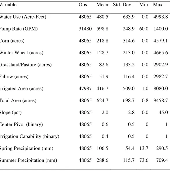
Table 1: Summary Statistics
Variable Obs. Mean Std. Dev. Min Max
Water Use (Acre-Feet) 48065 480.5 633.9 0.0 4993.8
Pump Rate (GPM) 31480 598.8 248.9 60.0 1400.0
Corn (acres) 48065 218.8 314.6 0.0 4579.1
Winter Wheat (acres) 48065 128.7 213.0 0.0 4665.6 Grassland/Pasture (acres) 48065 82.6 133.2 0.0 2902.9
Fallow (acres) 48065 51.9 116.4 0.0 2982.7
Irrigated Area (acres) 47987 416.7 509.0 1.0 8080.0
Total Area (acres) 48065 624.7 698.7 0.8 9458.7
Slope (pct) 48065 2.0 2.8 0.0 45.0
Center Pivot (binary) 48065 0.6 0.5 0 1
Irrigation Capability (binary) 48065 0.4 0.5 0 1 Spring Precipitation (mm) 48065 106.5 54.4 13.7 290.5 Summer Precipitation (mm) 48065 288.6 115.7 73.6 709.4
Table 1 summarizes the data used in the empirical analysis. The summary statistics include two variables which relate to overall farm size. ‘Irrigated Area’ was reported by the actual farmers in the water use data. ‘Total area’ is the physical area of every PLSS section operated by a given farmer. Total area is fixed, while irrigated area is possibly chosen by the
farmer, and should always be less than the total area due to legal restrictions. Total area is
exogenous to planting decisions, as opposed to irrigated area, which can be chosen by the farmer each year. An additional table of summary statistics (table 2), splits observations into three equal size groups. The groupings split observations between low, medium and high reported pumping capacities. The summary statistics reveal acute distinctions between the pumping capacity classes. Producers in the highest pumping capacity class, 714- 1400 gallons per minute, have the highest average water use, and highest irrigated area. The averages reveal that high capacity producers tend to apply more groundwater per acre, and tend to irrigate a higher portion of their farms’ total area. Producers in the lowest third of pumping capacities, which ranged from 60 – 490 gallons per minute, operate their wells for more hours, and dedicate more acreage to less water intensive uses, including wheat, fallow and sorghum. The summary statistics reveal a strong positive correlation between pumping capacities, and the number of acres devoted to corn. Simple pairwise comparisons were used to test for statistical differences between the group means. Every variable in the table below showed significant differences in means between the pumping capacity groupings at least at the one percent level.
Table 2. Summary statistics, grouped by pumping capacity tercile. PUMPING CAPACITY
60 - 490 GPM 490 - 715 GPM 714 - 1400 GPM
Water Pumped, acre-feet 301.2 479.9 569.2
Irrigated Area, acres 315.6 415.9 466.2
Total Area, acres 566.0 620.6 629.3
Hours Pumped 1626.3 1306.3 1060.7
Corn, acres 154.9 221.2 251.1
Winter Wheat, acres 147.8 125.7 101.0
Grassland, acres 84.9 82.8 75.1
Fallow Cropland, acres 67.3 50.6 32.4
Sorghum, acres 53.9 42.6 38.1
Soybeans, acres 10.9 30.5 57.6
Alfalfa, acres 16.2 29.0 24.5
The first step of the empirical analysis is to model the pumping capacities from Kansas’s water use records. Pumping capacities are critical to the analysis, as they explain the link
between physical aquifer characteristics and groundwater extraction quantities. Pumping capacity constraints motivate this linkage, whether or not farmers optimize groundwater extraction dynamically across multiple growing seasons. The goal in this stage is to create an instrument for the pumping capacity, and to check whether the recorded pumping capacities are consistent with hydrologic science. Over time, pumping capacities have been gradually
declining. Although farmers reported pumping capacities that varied substantially from year to year, only time-invariant explanatory variables are used in the regression. As a result, the model simply predicts an average pumping capacity for a given area. Parameters were estimated by the following model:
Pump Rateit = β0 + β1-2*Conductivity Classi + β3-5*Saturated Thickness Classi + β6*Latitudei + β7*Longitude + eit
The model is estimated by ordinary least squares, and the results show that pumping capacities are positively correlated with conductivity and saturated thickness. The coefficient estimates for each ‘bin’ of these two categorical variables have increasingly large magnitudes. The explanatory variables were explicitly chosen to identify the model. Over time, there could be an endogenous relationship between saturated thickness, and well pumping capacities. Here,
saturated thickness estimates predate the study period by 10 years, eliminating any potential feedback between these two variables.
Table 3: Statistical results for the pumping capacity model.
Dependent Variable: Pump Rate (GPM)
VARIABLES Coefficient Std. Error Significance
Conductivity: 50 to 100 ft./day 31.54 (3.555) *** 100+ ft./day 38.93 (3.833) *** Saturated Thickness 1997: 100 – 200 ft. 98.51 (2.927) *** 200 – 400 ft. 170.5 (4.210) *** 400 – 600 ft. 255.4 (16.07) *** Latitude -56.86 (2.018) *** Longitude 50.39 (1.080) *** Constant 7,735 (107.2) *** Observations 29,057 R-squared 0.248 *** p<0.01, ** p<0.05, * p<0.1
The variables latitude and longitude were included to allow for directional trends in pumping capacities. Their coefficient estimates translate to the highest average pumping capacities in South-East Kansas. The Southern component makes sense, given that the deepest parts of the Ogallala sit under Kansas’ Southern border with Oklahoma. The Eastern directional trend suggests climate might play a factor in well capacity, as Eastern Kansas receives
considerably more precipitation. Going from West to East, average summer precipitation roughly doubled in the parts of Kansas which overly the Ogallala.
The categorical variables are imprecise, yet their coefficient estimates exhibit directional trends that are consistent with hydrologic science. Additionally, the model’s predictions can be used to instrument for pumping capacities in further regressions. The instrumental variables approach overcomes the possibility of biased estimates that might result from measured well capacity being an endogenous explanatory variable. Using instrumental variables clears up this issue of causality.
The ultimate goal of the empirical analysis is to calculate the effect of pumping capacity on water and land use decisions. Ideally, we would use pumping capacity as an explanatory variable. However, farmers can potentially influence their own pumping capacity, either by setting their well’s pumping rate lower than its maximum capacity, or by excessive pumping that causes well capacity loss. As a result, pumping capacity cannot itself be used as an explanatory variable, as it is potentially correlated with the models’ error. To circumvent this problem, an instrument is needed to replace pumping capacity as an explanatory variable. The instrument must be highly correlated with pumping capacities and not directly influence the dependent variable. The aquifer parameters saturated thickness and conductivity serve as instruments for pumping capacity. The crux of this approach is that these aquifer characteristics only influence the dependent variables through their effect on pumping capacities.
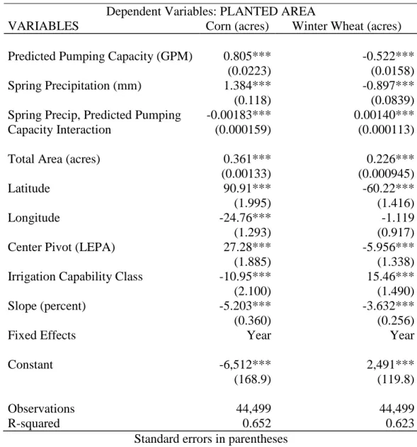
The next set of regressions regard the farmer’s crop mix decision. In two separate regressions, the number of acres planted with corn and wheat are used as dependent variables. These two crops are by far the most prevalent in Kansas, and are an important signal of how much water a farmer intends to use. Corn is more water intensive than wheat, and almost always
requires irrigation in Kansas. Wheat is less water intensive, but it is still common to irrigate wheat in Kansas. Acreage devoted to each crop was estimated using the following functional form:
Acreagejit = β0 + β1*𝑃𝑃𝑆𝑆𝑃𝑃𝑃𝑃 𝑅𝑅𝑎𝑎𝑆𝑆𝑆𝑆� i + β2*Spring Precipit+ β3*Spring Precipit*𝑃𝑃𝑆𝑆𝑃𝑃𝑃𝑃 𝑅𝑅𝑎𝑎𝑆𝑆𝑆𝑆� i + β4*Total Areait+ β5*Latitudei+ β6*Longitudei + β7*Center Pivoti+ β8*Irr. Capability Classi + β9*Slopei + β10-16*Year Fixed Effectst + eit
Subscripts jit indicate the number of acres of crop j, planted by farmer i, in year t. The first independent variable is the predicted pumping capacity estimated in the previous regression. An interaction term allows the effect of spring precipitation on pumping quantities to vary depending on the farm’s pumping capacity. Total area is included to allow for a scale effect, based on the overall size of the farm. Latitude and longitude allow for directional trends in planting decisions which occur due to climatic trends. Finally, the year fixed effects are meant to capture the influence of spatially invariant factors. For instance, the theoretic model predicts that relative prices influence the planting decision, yet in our analysis we are unable to observe prices that vary over space as well as time.
The empirical results are consistent with the model of water constrained producers. Predicted pumping capacities have a statistically significant impact on the number of acres allocated to corn and wheat. Higher pumping capacities correspond to more acres planted with corn, and less acres planted with wheat. These results are intuitive given that corn yields are more responsive to irrigation, and corn requires more irrigation. The results suggest that producers with greater irrigation capacity tend to plant more water intensive crops.
Table 4: Statistical results from the acreage allocation models.
Dependent Variables: PLANTED AREA
VARIABLES Corn (acres) Winter Wheat (acres)
Predicted Pumping Capacity (GPM) 0.805*** -0.522***
(0.0223) (0.0158)
Spring Precipitation (mm) 1.384*** -0.897***
(0.118) (0.0839)
Spring Precip, Predicted Pumping Capacity Interaction
-0.00183*** (0.000159)
0.00140*** (0.000113)
Total Area (acres) 0.361*** 0.226***
(0.00133) (0.000945)
Latitude 90.91*** -60.22***
(1.995) (1.416)
Longitude -24.76*** -1.119
(1.293) (0.917)
Center Pivot (LEPA) 27.28*** -5.956***
(1.885) (1.338)
Irrigation Capability Class -10.95*** 15.46***
(2.100) (1.490)
Slope (percent) -5.203*** -3.632***
(0.360) (0.256)
Fixed Effects Year Year
Constant -6,512*** 2,491***
(168.9) (119.8)
Observations 44,499 44,499
R-squared 0.652 0.623
Standard errors in parentheses *** p<0.01, ** p<0.05, * p<0.1
The Acres of corn variable is positively correlated with spring precipitation, while acres of wheat is negatively correlated with spring precipitation. Again, these results are intuitive, given that high initial soil moisture means that less irrigation will be required. The interaction term reveals that the impact of spring precipitation diminishes at higher predicted pumping capacities. In a dry spring, farmers with low pumping capacities tended to plant more acres of corn. Conversely, farmers with low pumping capacities showed less acres of wheat planted in a
wet spring. This result might seem puzzling, given that winter wheat recorded in the data had to be planted the previous fall. The negative relationship between acres of wheat and spring precipitation is probably due to the way the NASS data was recorded. In a wet spring, farmers were more likely to follow wheat with a crop of soybeans. In the data, double-cropped acres are treated as their own distinct crop, and thus results in less overall area regarded as wheat.
The potential for double cropping might also explain directional planting trends captured in the latitude and longitude variables. The directional trends indicate that corn is preferred in the North-West (since longitude is always negative in the sample), and that wheat is preferred
towards the South, conditional on the model’s other explanatory variables. Southern regions of Kansas have a longer growing season, and therefore farmers have a greater potential to establish winter wheat after corn has been harvested.
Of the remaining variables included in these regressions, total area, center pivot, and slope had coefficient estimates of the expected signs. The coefficient estimate for irrigation capability class indicates that higher-quality soil is preferred for growing wheat.
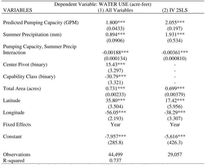
A final round of regressions considers the effect of pumping capacities on the actual quantity of water used by farmers. Regression equation 1 was fit according to the following functional form:
Water Useit= β0+ β1* 𝑃𝑃𝑆𝑆𝑃𝑃𝑃𝑃 𝑅𝑅𝑎𝑎𝑆𝑆𝑆𝑆� it+ β2*Summer Precipit + β3*𝑃𝑃𝑆𝑆𝑃𝑃𝑃𝑃 𝑅𝑅𝑎𝑎𝑆𝑆𝑆𝑆� it*Summer Precipit
+ β4*Center Pivoti + β5*Capability Classi + β6*Total Areait + β7*Latitudei + β8*Longitudei+ β9-15*Year Fixed Effectst + eit
In a second specification, (regression equation 2), the center pivot and soil capability class variables are omitted. The primary difference in the second specification is use of the
stage least squares (2SLS) instrumental variables estimation technique. In the first regression, pumping rates were estimated for every well in the sample using the coefficient estimates presented in table 3. The second regression omits observations that did not include the pumping rate field. Although this decreases the sample size, it allows usage of two-stage least squares estimation. As a result, the standard errors for the pumping rate variables are larger in equation 2. Coefficient estimates are slightly different between the two equations, but the interpretation of the results remains unchanged between the two specifications.
Table 5. Statistical Results for the water use regression.
Dependent Variable: WATER USE (acre-feet)
VARIABLES (1) All Variables (2) IV 2SLS
Predicted Pumping Capacity (GPM) 1.800*** 2.055***
(0.0433) (0.197)
Summer Precipitation (mm) 0.894*** 1.931***
(0.0906) (0.534)
Pumping Capacity, Summer Precip
Interaction -0.00188*** -0.00361***
(0.000134) (0.000810)
Center Pivot (binary) 15.43*** -
(3.297) -
Capability Class (binary) -30.79*** -
(3.321) -
Total Area (acres) 0.731*** 0.699***
(0.00233) (0.00379)
Latitude 35.80*** 17.42***
(3.504) (5.956)
Longitude -56.05*** -38.29***
(2.193) (3.307)
Fixed Effects Year Year
Constant -7,957*** -5,616***
(285.8) (426.3)
Observations 44,499 29,057
R-squared 0.737
Standard errors in parentheses, *** p<0.01, ** p<0.05, * p<0.1 31
Results from the water use regression confirm the importance of well capacity
constraints. Predicted pumping capacities had a positive and significant impact on the amount of water used. At first glance, it may appear that summer precipitation has the incorrect sign. Precipitation should have a negative sign, since precipitation should decrease the amount of irrigation that is needed. The interaction term clears up this confusion. When the negative interaction coefficient is multiplied by a farms’ pumping capacity, the marginal impact of a millimeter of rain is almost always negative. Farms with extremely low pumping capacities tended to apply more water, on average, as a result of precipitation. In years with high precipitation, farms with high pumping capacities cut back on the amount of water used.
VI. CONCLUSION
In the Western United States, and many other parts of the world, groundwater is being used faster than it is being replenished. Farmers know that declining groundwater reserves will also mean lower well capacities. Despite these facts, very few economic models of groundwater use feature constraints that can limit the amount of water consumed. This thesis makes the case that supply constraint are indeed relevant, and are important to, groundwater use decisions. This argument was made using theoretical and empirical methods. The theoretical model showed how aquifer characteristics can influence water use decisions. By omitting this relevant feature, previous theoretical work likely reached misguided conclusions, which often were not supported by empirical results. In contrast, this paper’s empirical results broadly support the theoretical models’ predictions. Pumping capacities exhibited the expected relationships with planting decisions and overall water use.
A key result of the empirical analysis is the effect of precipitation on water use decisions. Farms with low well capacity showed less responsiveness to seasonal precipitation. This result may be driven by these farms’ reactions to high or low precipitation. In dry years, low well capacity can constrain the amount of groundwater available for irrigation. In years with above average precipitation, low capacity farmers are likely to be reluctant to curtail groundwater pumping. These farmers know that they cannot adequately meet crop water requirements at the peak of summer, when corn yields are most sensitive to water stress. As a result, they utilize the soil’s ability to store water in order to bank soil moisture for this critical period. Low capacity users adapt strategies such as pre-irrigating fields before planting, and continuing to irrigate during the rain. On the other hand, farmers with adequate pumping capacity can turn off
irrigation systems when it rains, and save on pumping costs, knowing that they will have an adequate supply of groundwater later on in the season to meet crop-water requirements.
These results have broad implications. Economic models which accurately depict the decisions of irrigators do a better job of explaining water use outcomes. For example, many economic studies have estimated very low responsiveness of water use to factors which should influence the profits associated with irrigation. Depth to water strongly impacts the costs of pumping, yet few studies are able to show a negative correlation between pumping depth and extraction quantities. Low elasticity of groundwater demand has also stymied attempts to curb groundwater extractions in Colorado’s San Luis basin. For many farmers there, irrigation remains attractive, even when it comes with an extremely high bill.
Economists should reevaluate the potential gains from groundwater management, in light of well capacity constraints. On the High Plains, groundwater is being used where it is available, and not necessarily where it is the most valuable. This thesis presented evidence that a myopic water use strategy is able to predict water use decisions in Kansas. This does not mean
stakeholders in Kansas never dynamically balance water use decisions over many years. However, it suggests that Kansas’ groundwater is largely a common-pool resource. Lacking complete ownership, groundwater users’ personal incentives do not align with social objectives.
Groundwater supply constraints imply that access to groundwater is not a binary
outcome. When policymakers consider enacting homogenous policies, farmers take into account what it will mean for them, given their circumstances. Economists favor incentive based policies as an efficient way to influence resource use. Unlike command and control policies, the
effectiveness of policies such as tradable quotas depends on how groundwater users’ respond to
them. Well capacity constraints may affect which types of policies are most likely to be enacted and how those policies should be designed.
On the High Plains, policymakers are looking for ways to reduce annual groundwater use and extend the life of the aquifer. A natural extension to this research project would be to design a policy in light of well capacity constraints, which is both palatable to groundwater users, and effective. A dynamic model of groundwater extraction could provide the theoretical framework to predict which types of groundwater users are more receptive of groundwater management. A survey of groundwater users on the High Plains could provide the means to tie attitudes about conservation to spatial aquifer characteristics.
Future research could examine crop insurance subsidies in light of heterogeneous well capacities. The United States federal government backs insurance for irrigated crops, which provides economic relief to farmers in times of drought. Crop insurance payouts are made on a per-acre basis, making it easy to see how subsidized crop insurance skews incentives towards planting water intensive crops. If the insurance policies do not accurately reflect differences in well capacity, it will likely lead low capacity farmers to knowingly overplant corn. Crop insurance subsidies likely reduce the efficiency of economic output per unit of groundwater irrigation. In order to receive an insurance payout, farmers must demonstrate that they attempted to irrigate the crop to the best of their ability. Therefore farmers might continue irrigating after losing all hope of raising a successful crop.
In the shorter term, the next steps for this research take the form of minor refinements. In particular, a well’s depth to water is another potentially important variable that is omitted from these regressions. The impact of depth to groundwater has been featured in many economic studies, such as Hendricks and Peterson (2012) and Pfeiffer and Lin (2014b). In contrast, Foster
et al. (2015) makes the argument that pumping capacities can be a more important driver of water use decisions than depth to water. Depth to water should be positively correlated with well pumping rates, through its impact on groundwater recharge. Theoretically, depth to water should be negatively correlated with groundwater pumping, although in Kansas, groundwater pumping has permanently lowered groundwater levels. As a result, the areas that historically have used the most groundwater now experience the greatest depth to water.
A second refinement will be to analyze water use per acre irrigated. The original
intention of this project was to calculate water use intensity on a per-crop basis, using the NASS land cover data. Unfortunately, a convincing instrument for the crop variables did not
materialize, meaning they could not be completely identified in a statistical model. A follow-up study will analyze water use per acre authorized for irrigation. The authorized acres variable is strictly exogenous, and should provide means to study the intensity of water use across well capacities.
Crop yields are an additional key piece of information that were not available for this study. If low capacity users apply less water per acre irrigated, their yields will be negatively impacted. The data used in this study did not include crop yields, which limits the ability to draw conclusions about water use on the High Plains. Crop yield data is available at the county level, from the National Agricultural Statistics Service, however county level statistics are likely too broad to tease out the effect of well capacity on crop yields. NASA’s Landsat satellite imagery might provide future research with the means to collect data on crop yields at the individual field level. Infrared satellite images, such as the Normalized Difference Vegetation Index (NDVI) can be used to calculate a crops’ canopy temperature, a key indicator of water stress. If crop water
stress is more prevalent in areas with low well capacity, it would bolster the argument that well capacity constraints have an important influence on water use decisions.
In this thesis, groundwater well pumping capacity was modelled in a theoretical framework, and in an empirical setting using observational data. The theoretical model of groundwater supplied producers was supported by groundwater usage records from Kansas. Use of a novel data source tied farmers’ crop decisions to water use outcomes at an unprecedented level of clarity. We found that regions with more available groundwater planted a more water intensive crop mix, and used more water on average. These results substantiate the economic model of capacity constrained groundwater users.
VII. REFERENCE LIST
Anderson, S. T., Kellogg, R., & Salant, S. W. (2014). Hotelling under pressure. (No. w20280). National Bureau of Economic Research.
Brozović, N., Sunding, D. L., & Zilberman, D. (2006). Optimal Management of Groundwater over Space and Time. Frontiers in Water Resource Economics, 109-135.
Brozović, N., Sunding, D. L., & Zilberman, D. (2010). On the spatial nature of the groundwater pumping externality. Resource and Energy Economics, 32(2), 154-164.
Fitzgerald, T., & Zimmerman, G. (2013). Agriculture in the Tongue River Basin: Output, Water Quality, and Implications. Agricultural Marketing Policy Paper, No. 39.
Foster, T., Brozović, N., & Butler, A. P. (2014). Modeling irrigation behavior in groundwater systems. Water Resources Research, 50(8), 6370-6389.
Foster, T., Brozović, N., & Butler, A. P. (2015). Analysis of the impacts of well yield and groundwater depth on irrigated agriculture. Journal of Hydrology, 523, 86-96.
Gardner, M., Moore, M., & Walker, J. (1997). Governing A Groundwater Commons: A Strategic and laboratory analysis of western water law. Economic Inquiry. 35: 218-234.
Gisser, M., & Sánchez, D.A. (1980). Competition versus optimal control in groundwater pumping, Water Resources Research. 16(4), 638–642.
Guilfoos, T., Pape, A. D., Khanna, N., & Salvage, K. (2013). Groundwater management: The effect of water flows on welfare gains. Ecological Economics, 95, 31-40.
Hardin, G. (1968). The tragedy of the commons. Science, 162(3859), 1243-1248.
Hecox, G., Macfarlane, P., Wilson, B. (2002) Calculation of Yield for High Plains Wells:
Relationship between saturated thickness and well yield. Kansas Geological Survey Open
File Report 2002-25C. Retrieved from
http://www.kgs.ku.edu/HighPlains/OHP/2002_25C.pdf
Hendricks, N.P., & Peterson, J.M. (2012). Fixed effects estimation of the intensive and extensive margins of irrigation water demand. Journal of Agricultural and Resource
Economics, 37(1), 1.
Hendricks, N. P., Sinnathamby, S., Douglas-Mankin, K., Smith, A., Sumner, D. A., & Earnhart, D. H. (2014). The environmental effects of crop price increases: Nitrogen losses in the US Corn Belt. Journal of Environmental Economics and Management, 68(3), 507-526. Koundouri, P., (2004). Current Issues in the Economics of Groundwater Resource Management.
Journal Of Economic Surveys. 18: 703–740.
Pfeiffer, L., & Lin, C.Y.C. (2012). Groundwater pumping and spatial externalities in agriculture.
Journal of Environmental Economics and Management, 64(1), 16-30.
Pfeiffer, L., & Lin, C.Y.C. (2013). Property rights and groundwater management in the High Plains Aquifer. Working paper, University of California at Davis.
Pfeiffer, L., & Lin, C.Y.C. (2014a). Does efficient irrigation technology lead to reduced
groundwater extraction? Empirical evidence. Journal of Environmental Economics and Management, 67(2), 189-208.
Pfeiffer, L., & Lin, C. Y. C. (2014b). The Effects of Energy Prices on Agricultural Groundwater Extraction from the High Plains Aquifer. American Journal of Agricultural Economics. Retrieved from http://ajae.oxfordjournals.org/content/early/2014/05/15/ajae.aau020.short. PRISM Climate Group, Oregon State University, http://prism.oregonstate.edu, created 4 Apr
2015.
Provencher, B., & Burt, O. (1993). The externalities associated with the common property exploitation of groundwater. Journal of Environmental Economics and
Management, 24(2), 139-158.
Scheierling, S.M., Loomis, J.B., Young, R.A., (2006). Irrigation Water Demand: A Meta-Analysis of Price Elasticity. Water Resouces Research. 42: 1-9.
Schneekloth, J.P. (2015) Cropping Rotations Using Limited Irrigation. Procedings of the 27th
Annual Central Plains Irrigation Conference. Retrieved from
http://www.ksre.ksu.edu/pr_irrigate/OOW/P15/Lamm15_IrrSched.pdf.
Scheenkloth, J.P. (2012) Irrigation Capacity Impact on Limited Irrigation Management and Cropping Systems. Procedings of the 24th Annual Central Plains Irrigation Conference.
Retrived from http://www.ksre.ksu.edu/pr_irrigate/OOW/P12/Schneekloth12.pdf. Suter, J.F., Duke, J.M., & Messer, K.D. (2012). Behavior in a Spatially Explicit Groundwater
Resource. American Journal of Agricultural Economics. 94(5): 1094-1112.
Theis, C. V. (1935). The relation between the lowering of the Piezometric surface and the rate and duration of discharge of a well using ground‐water storage. Eos, Transactions American Geophysical Union, 16(2), 519-524.
Todd, D. K., & Mays, L. W. (2005) Groundwater Hydrology. Hoboken, NJ: John Wiley & Sons. Weight, W. D., & Sonderegger, J. L. (2001) Manual of Applied Field Hydrogeology. New York:
McGraw-Hill. Print.
Appendix 1. SATELLITE DATA AND GIS PROCEDURES
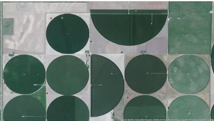
Figure 4: Center Pivot Irrigation Systems in Kanas.
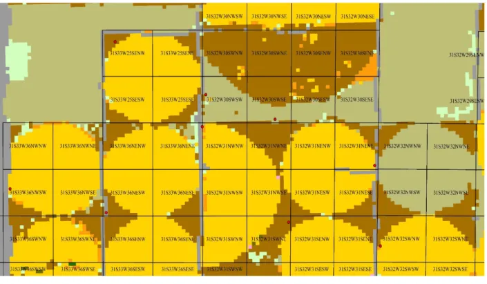
Figure 5: Public Land Survey System (PLSS) ‘Quarter Quarter’ Sections
Figures A.1 and A.2 show a satellite image of center-pivot irrigation systems in Kansas. The red dots are the spatial location of wells from Kansas’ water use records. In figure A.2, a grid of PLSS ‘Quarter Quarter” sections overlays the satellite image. Each square section is approximately 40 acres. The smaller circles are inset into a full quarter section, and are the most frequently sized irrigation system. These systems irrigate an approximately 120 acre circle within the full 160 acre Quarter section.
Figure 6: Crop Cover Data
Figure A.3 shows the National Agricultural Statistic Services’ (NASS) Crop-Cover data for the same area. Each square pixel in the ‘Raster’ data represents a 30 by 30 meter area;
equivalent to about a quarter of an acre. Each pixel is colored by its crop code. Yellow represents corn, brown represent wheat, and the greenish tan color represents grassland.
The crop cover data was relayed to the farmer level water-use data in several steps. Each well was authorized to irrigate an average of four PLSS sections. The wells were grouped by
farmer, and the wells were used to map the PLSS sections to the farmer. Finally, the raster data was aggregated by farmer using GIS software. The area of each crop is simply calculated as the number of pixels assigned to each crop code, multiplied by the area of one pixel (900 m2).
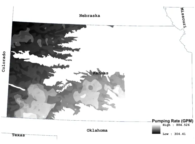
Figure 7: Predicted Pumping Rates in Kansas, 2006-2013.
Figure A.4 is a visual representation of the results from the pumping-rate regression. In the figure, shaded regions show the High Plains Aquifer’s extent in Kansas. The lighter regions show areas with higher pumping rates, which are largely driven by saturated thickness, and the directional trends. Eastern Kansas receives more precipitation, and the aquifer is closer to the land surface, both of which contribute to potential recharge.