A fatigue analysis including
environ-mental effects for a pipe system
in a Swedish BWR
2011:30
Author: Kristin SteingrimsdottirMagnus Dahlberg
SSM perspective
Background
The effect of the environment on fatigue design has been the subject of intense study in USA, Japan and elsewhere. Several reports indicate a potentially large influence of the environment, leading to the proposal of entirely new analysis procedures. SSM has in an earlier project spon-sored research to evaluate the technical basis for these proposals, see SSM Research Report 2011:04. In the current report, the consequences for a Swedish BWR piping system are evaluated using the new analysis procedure including environmental effects on fatigue.
Objectives
The principal objective of the project has been to find out the conse-quences for a Swedish BWR piping system using the new analysis proce-dure to include environmental effects on fatigue. Another objective has been to find out how well the commercial code Pipestress can handle environmental effects on fatigue.
Results
• Introducing the new NUREG/CR-6909 procedure in fatigue assess-ments will add substantial complexity to the analysis procedure. • The stainless steel pipe system, with moderate usage factor U = 0.2,
will have a usage factor of 0.9 after 60 years when both a new fatigue curve and an environmental correction factor Fen are considered. • If maximum temperatures are combined with average strain rates
the correlation between the results from Pipestress and the detai-led method is quite good. Conservatism in relation to the detailed method is obtained if lower bound strain rates are used as input instead of mean values.
• The model examples show the importance of the temperature values for the computed Fen values. The strain rate is of less im-portance, however not negligible.
• The environmental factors were larger for the ferritic steel piping than for the austenitic steel piping by a factor to the order of 2-2.5 for identical transients.
• Pipestress, with its current implementation for environmental factors, should not be used as a research tool for environmental effects on fatigue. However, Pipestress can be used as an effective tool for considering environmental effects in an engineering fati-gue analysis of piping systems. It is then recommended that the maximum transient temperature is always chosen for input. Need for further research
The results are important in order to make relevant fatigue assessments of nuclear components in reactor water environments. More research is needed for the further investigation of the best way to include environ-mental effects in fatigue analysis, both for design and for evaluating the risk of fatigue failure of ageing nuclear components.
2011:30
Authors: Kristin Steingrimsdottir and Magnus Dahlberg, Inspecta Technology AB, Stockholm, Sweden
A fatigue analysis including environ-
mental effects for a pipe system
in a Swedish BWR
This report concerns a study which has been conducted for the Swedish Radiation Safety Authority, SSM. The conclusions and
view-Table of content
1. Summary ... 2
2. ANL vs. ASME ... 3
3. Environmental fatigue life correction factor (Fen) ... 5
3.1. The method of computing Fen and the usage factor ... 5
3.2. Fen applied on a realistic BWR system with the NUREG 6909 method ... 7
4. Conclusions ... 12
5. References... 13
Appendix A ... 14
A1. Nomenclature ... 15
A2. Pipe system and loading ... 16
A2.1. Pipe system ... 16
A2.2. Load cases ... 17
A3. Environmental fatigue life correction factor (Fen) ... 19
A3.1. The Inspecta method of computing Fen and the usage factor according to NUREG/CR-6909 ... 19
A3.2. The method of computing Fen and the usage factor according to Pipestress ... 20 A4. Data ... 23 A5. Result ... 24 A6. Conclusions ... 30 A7. References ... 31
1. Summary
A BWR feed water piping system (austenitic steel) has been analyzed with two different fatigue curves and environmental factors. Original fatigue curve from ASME is compared to a new fatigue curve; ANL. The influence of environmental correction factors (Fen) is studied further for the piping
system. It is noted that the results apply for this particular system, and gen-eral conclusions should be cautiously drawn. Typical for this system is that all dominant loads are within the low-cycle regime. This implies that the change of fatigue curve only leads to limited increases in usage factors. Larger changes can occur if larger number of cycles is within the high-cycle regime.
The new fatigue curve ANL increases the usage factor to the order of 50-100% for a system with dominant low cycle fatigue
The influence of the environmental correction factor is substantial, about 300% on the usage factor
The results indicate that the environmental factor should be fairly independent of the location in the system. This result is of practical importance, but should however need further study to be confirmed.
Combining the two effects, this system with moderate usage factor
U=0.2, will have a usage factor of 0.9 after 60 years.
Introducing the NUREG/CR-6909 procedure in fatigue assessments will add substantial complexity to the calculation procedure.
Implementation of the procedure in commercial codes would be very help-ful. However, the procedure is not clearly described. Hence, the implementa-tion should be examined closely and evaluated before being universally in-troduced in applications.
Therefore, the implementation for the environmental factor, Fen, in the
com-mercial analysis program Pipestress has been investigated in an appendix to the present report. The investigation was carried out by analysis with three transients on a model piping system. The Pipestress results were compared with results obtained by the detailed procedure, based on the instructions in NUREG/CR-6909. The comparisons were performed for austenitic and fer-ritic steels.
The implementation of the environmental factor computation in Pipestress is simple. No detailed integration with time varying parameters is per-formed. Instead all parameters remain constant throughout the transients.
The parameter values are given as default by Pipestress unless other values are provided by the analyst.
The comparison shows that these constant parameter values for Pipestress must be chosen with care in order to obtain results comparable to those ob-tained by the detailed calculations.
Calculations with mean transient temperature values as input should be avoided, since the environmental factors tend to become significantly
low-er than the values dlow-erived by the detailed calculations. Instead maximum transient temperatures should be used as input.
If maximum temperatures are combined with average strain rates the cor-relation between Pipestress and the detailed method is surprisingly good. Clear conservatism in relation to the detailed method is obtained if lower bound strain rates are used as input instead of mean values.
These model examples show the importance of the temperature values for the computed Fen values.
The strain rate is of less importance, however not negligible.
The local stress indices K3, raise the stress ranges up to three times the
value for a straight pipe. However, this only results in 15-30 % increase of the Fen value. Hence, the computed Fen is fairly independent of the
compo-nent type.
The environmental factors were larger for the ferritic steel piping than for the austenitic steel piping by a factor to the order of 2-2.5 for identical transients.
Pipestress with its current implementation for environmental factors should not be used as a research tool for environmental effects. However, Pipestress can be used as an effective tool for considering environmental effects in the engineering analysis of piping systems. It is recommended that the maxi-mum transient temperature is always chosen for input.
2. ANL vs. ASME
A Swedish class 1 BWR feed water piping system has been analyzed for 60 years of operation. The piping system is made of conventional austenitic stainless steel. The pipe system is originally modeled with Pipestress /3/ and the fatigue calculation in Pipestress is based on a fatigue curve from ASME. A new fatigue curve, ANL, from NUREG/CR-6909 /1/ is proposed that has a factor 12 on life and 2 on stress versus the ASME curve that has a factor of 20 on life and 2 on stress. Moreover, the mean data differ between the two design curves, which leads to the significant difference in the high cycle regime. See Figure 1 where the two fatigue curves are compared.
Figure 1: ASME compared to ANL fatigue curve
In all cases of fatigue calculations the ANL curve will lead to a higher usage factor than the ASME curve, see Figure 2 and Figure 3. The impact is most prominent for lower loads, but also for lower usage factors. The usage fac-tors are increased to order of 50% -100% for all the fatigue limiting loca-tions. The majority of the fatigue load is within the low-cycle fatigue regime.
0,00 0,05 0,10 0,15 0,20 0,25 0,30 0,35 0,00 0,05 0,10 0,15 0,20 0,25 0,30 0,35 UASME UANL 0 1 2 3 4 5 6 7 8 9 0,00 0,05 0,10 0,15 0,20 UASME UANL /U A SM E
Figure 2: Usage factor of ASME vs. usage factor of ANL Figure 3: Usage factor of ASME vs. the ratio of usage
3. Environmental fatigue life
correction factor (F
en
)
3.1. The method of computing F
en
and the usage factor
Appendix A in NUREG /1/ describes how to calculate Fen. Several
simpli-fied methods (presumably more conservative) exist, but Inspecta has chosen to use the most detailed method. For a transient the nominal Fen,nom is
calcu-lated for every time step in the transient.
) 734 , 0 exp( , TO
Fennom (1)For the whole transient the Fen is calculated with the modified rate approach
/1/.
n k k k k k en enF
T
F
1 max min ,(
,
)
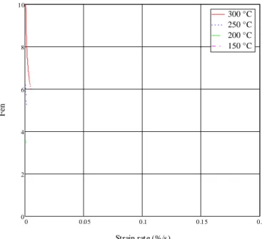
(2)The environmental correction factor changes with temperature and strain rate, see Figure 4. The value of Fen is sensitive to temperature especially at
low strain rate. Also it can be noticed is that the Fen is discontinuous, i.e.
jumps from 1 to 2.08 as soon as the conditions applies.
0 0.05 0.1 0.15 0.2 0 2 4 6 8 10 300 °C 250 °C 200 °C 150 °C Strain rat e (%/s) F en
The procedure for calculating Fen in real cases needs some clarifications. As
indicated by Eqn. 1, Fen is obtained by integrating over the strain. A unique
value of Fen is obtained for each stress range. See the example in
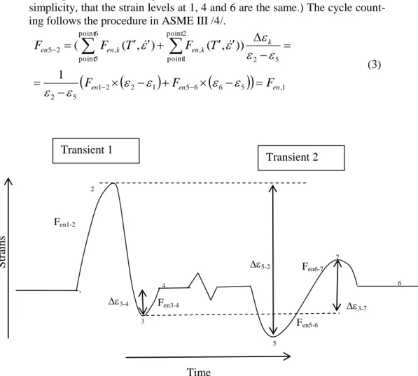
Figure 5 and Equation 3. The combination of the two transients in the figure sums up to two strain ranges, and (It is assumed, for
simplicity, that the strain levels at 1, 4 and 6 are the same.) The cycle count-ing follows the procedure in ASME III /4/.
1 2 2 1 5 6 6 5
,1 5 2 5 2 6 point 5 point 2 point 1 point , , 2 5 1 ) ) , ( ) , ( ( en en en k k en k en en F F F T F T F F
(3)Finally to evaluate the usage factor the sum of all usage factors on two tran-sients together are multiplied with the Fen for that combination of transient.
n en n i en i en en en en
U
F
U
F
U
F
U
F
U
F
U
1
,1
2
,2
3
,3
,...
, (4) See for example Asada /2/ for a more comprehensive description of the pro-cedure. The procedure used by Inspecta follows Asada and should be in agreement with international praxis. This has been confirmed in communica-tion with other internacommunica-tional organizacommunica-tions (NRC, TVO, etc,) involved in the study of environmental effects.Figure 5: Two transients, strain as a function of time
5-2 3-4 3-7 Fen1-2 Fen3-4 Fen5-6 Fen6-7 1 2 4 5 6 7 3 Transient 1 Transient 2 Time Str ai ns
3.2. F
en
applied on a realistic BWR
system with the NUREG 6909
method
Current fatigue tools are not well suited for computing Fen. For this case the
strain rate is needed and that information is not accessible from Pipestress /3/ directly, in the revision available for Inspecta Technology during this work. Therefore ANSYS is used for modeling of the through the wall temperature gradient and extracting the corresponding stresses. Moment stresses are ob-tained by scaling the maximum moment, under the assumption that the mo-ment stresses vary linearly with the average wall temperature. The stresses due to the pressure are obtained directly from the pressure given in the load definition.
The node in the pipe system that had the highest usage factor is studied fur-ther. At the node Fen was computed for the dominant transients. This node
has a computed usage factor from Pipestress /3/; UASME=0.2 and with the
ANL curve the usage factor gave; UANL=0.3.
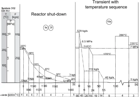
Pipestress /3/ gives usage factor for two transients together. These transients are simulated with a small axisymmetric straight pipe model in ANSYS. Only temperature transients are modeled with ANSYS. The stress from pres-sure is calculated separately and stress from moment is calculated by lineari-zation. For a linear transient in temperature a certain value for the moment is obtained from Pipestress /3/ that will give a linear response in accordance to the mean temperature in the pipe model. The sum of stresses from thermal, moment and pressure are used to calculate the total strain, and from that the strain rate is obtained, see equations (5) and (6). Figure 6 shows a transient combination and Figure 7 shows the strain vs. time for that specific transient combination. E pressure moment thermal total
(5)t
total total
(6)Figure 6: Transients 9a29 and 16e, that combine to Fatigue cycle 6.
Figure 7: Time vs. strain (Transients 9a29 and 16e), Fatigue cycle 6
Reactor shut-down Transient with temperature sequence -3,5E-01 -3,0E-01 -2,5E-01 -2,0E-01 -1,5E-01 -1,0E-01 -5,0E-02 0,0E+00 5,0E-02 1,0E-01 1,5E-01 0 4000 8000 12000 16000 Time [s] S tr a in [ % ] -3,5E-01 -3,0E-01 -2,5E-01 -2,0E-01 -1,5E-01 -1,0E-01 -5,0E-02 0,0E+00 5,0E-02 1,0E-01 1,5E-01 11000 12000 13000 14000 15000
Reactorshut-down Temperature
Many of the fatigue cycles that are applied, see Table 1, have the 16c transi-ent that gives about 4 in the Fen value. The other fatigue cycles that also
re-sults in a higher value of Fen is cycle 2 (transient 9a29 and 16f) and cycle 27
(transient 16e and 16d). They give a Fen little over 4. Other transient
combi-nations do not give as high value for Fen.
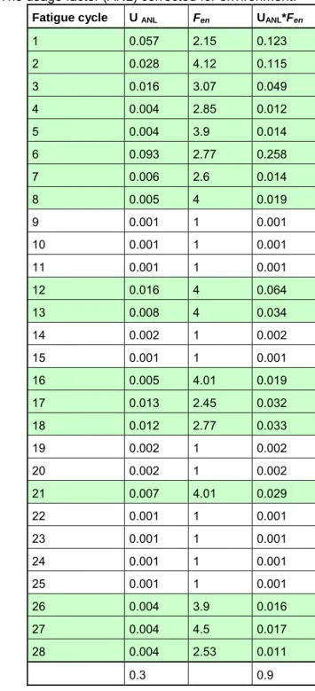
Table 1: The usage factor (ANL) corrected for environment.
Fatigue cycle U ANL Fen UANL*Fen
1 0.057 2.15 0.123 2 0.028 4.12 0.115 3 0.016 3.07 0.049 4 0.004 2.85 0.012 5 0.004 3.9 0.014 6 0.093 2.77 0.258 7 0.006 2.6 0.014 8 0.005 4 0.019 9 0.001 1 0.001 10 0.001 1 0.001 11 0.001 1 0.001 12 0.016 4 0.064 13 0.008 4 0.034 14 0.002 1 0.002 15 0.001 1 0.001 16 0.005 4.01 0.019 17 0.013 2.45 0.032 18 0.012 2.77 0.033 19 0.002 1 0.002 20 0.002 1 0.002 21 0.007 4.01 0.029 22 0.001 1 0.001 23 0.001 1 0.001 24 0.001 1 0.001 25 0.001 1 0.001 26 0.004 3.9 0.016 27 0.004 4.5 0.017 28 0.004 2.53 0.011 0.3 0.9
The Fen factors for these dominant fatigue cycles give an increase about 215
– 450 %. The total usage factor will increase by a factor of 300 %, so the usage factor will be around 0.9. Note that the Fen has only been calculated
for the dominant transients, colored green, the others are assumed to have negligible influence on Fen. Inspectas results have been shown to
representa-tives from NRC (USA) and TVO (Finland, together with VTT), which have performed previous studies on environmental factors. When compared to other international studies on the environmental factor, it shows similar re-sults for the value of Fen. Note that Inspecta computed Fen independently,
separated from the stress ranges in Pipestress. Hence, the stress ranges in Inspectas computations and Pipestress may differ, at least slightly. In order to examine this, a stress raise factor, K, was applied to the total stress range. The calculations on Fen value are done with K factor equal to one. When
calculating the Fen value with K=2, Fen decreases 7 %. Hence doubling the
stress range had no substantial influence in this case. This indicates that the value of Fen should be rather independent of the location in the piping
sys-tem. This should, however, need a further study to be confirmed.
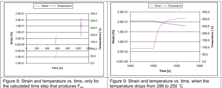
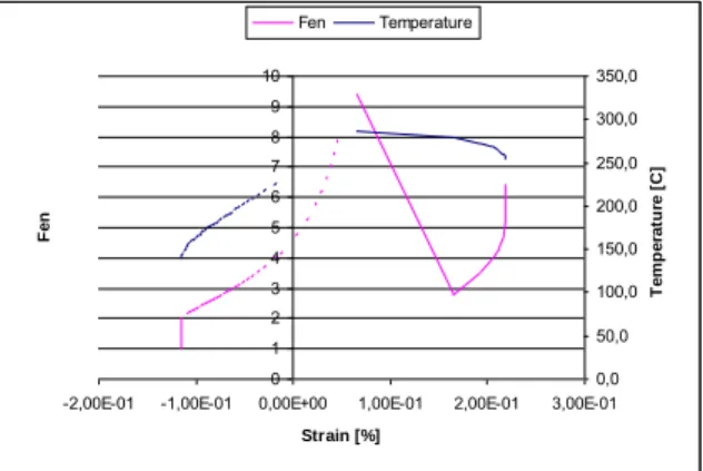
It is of interest to see what is contributing to high Fen values as in fatigue
cycle 13. In Figures 8 - 11, Fen and other contributing factors are graphically
displayed. See Figure 8 and Figure 9 for the strain and temperature interac-tion. Note how the strain increases with increased temperature and then how the strain rapidly increases when the temperature drops from 286 to 250 ˚C. In
Figure 10
andFigure 11
the environmental factor, Fen is plotted againstthe strain rate and the temperature and one can see how they affect the value of Fen. The strain rate, temperature and Fen are connected by equation (1)
-1,5E-01 -1,0E-01 -5,0E-02 0,0E+00 5,0E-02 1,0E-01 1,5E-01 2,0E-01 2,5E-01 0 200 400 600 800 1000 1200 Tim e [s] S tr a in [ % ] 0,0 50,0 100,0 150,0 200,0 250,0 300,0 350,0 T em p er at u re [ ˚C ] Strain Temperature 0,0E+00 5,0E-02 1,0E-01 1,5E-01 2,0E-01 2,5E-01 1045 1050 1055 1060 Time [s] S tr a in [ % ] 0,0 50,0 100,0 150,0 200,0 250,0 300,0 350,0 T e m p e ra tu re [ ˚C ] Strain Temperature
Figure 8: Strain and temperature vs. time, only for
the calculated time step that produces Fen
Figure 9: Strain and temperature vs. time, when the temperature drops from 286 to 250 ˚C
A closer look at Figure 10 and Figure 11 tells that there are three significant changes of Fen, initial increase, thereafter decrease and final increase. There
is an initial increase in temperature and a small decrease in strain rate till the
Fen value has reached its maximum value. Thereafter Fen decreases, probably
due to the increase in strain rate. The final increase of Fen seems to depend
primarily on the strain rate decrease. These figures readily show how the parameters temperature and strain rate simultaneously affect the value of Fen.
0 1 2 3 4 5 6 7 8 9 10
-2,00E-01 -1,00E-01 0,00E+00 1,00E-01 2,00E-01 3,00E-01
Strain [%] F e n -2,00E-02 0,00E+00 2,00E-02 4,00E-02 6,00E-02 8,00E-02 1,00E-01 1,20E-01 S tr a in r a te [ % /s ]
Fen Strain rate
0 1 2 3 4 5 6 7 8 9 10
-2,00E-01 -1,00E-01 0,00E+00 1,00E-01 2,00E-01 3,00E-01
Strain [%] F e n 0,0 50,0 100,0 150,0 200,0 250,0 300,0 350,0 T e m p e ra tu re [ C ] Fen Temperature
4. Conclusions
It is noted that the results apply for this particular system, and general con-clusions should be cautiously drawn. Typical for this system is that all domi-nant loads are within the low-cycle regime. This implies that the change of fatigue curve only leads to limited increases in usage factors. Larger changes can occur if larger number of cycles is within the high-cycle regime.
The new fatigue curve ANL increases the usage factor to the order of 50-100% for a system with dominant low cycle fatigue
The influence of the environmental correction factor is substantial, about 300% on the usage factor
The results indicate that the environmental factor should be fairly independent of the location in the system. This result is of practical importance, but should however need further study to be confirmed.
Combining the two effects, this system with moderate usage factor
U=0.2, will have a usage factor of 0.9 after 60 years.
Introducing the NUREG 6909 procedure in fatigue assessments will add substantial complexity to the calculation procedure.
Implementation of the procedure in commercial codes would be very helpful. However, the procedure is not clearly described. Hence, the implementation should be examined closely and evaluated before being universally introduced in applications.
5. References
/1/ Chopra, O. K, Shack, W. J., Effect of LWR Coolant Environments
on the Fatigue Life of Reactor Materials, NUREG/CR-6909,
ANL-06/08, 2007.
/2/ Asada, S., Proposal for determination of strain rate in
environ-mental fatigue correction evaluation, Proceedings of the ASME
2009 Pressure Vessels and Piping Division Conference, 2009. /3/ Pipestress, DST, Version 3.5.1.
/4/ ASME Boiler & Pressure Vessel Code, ASME III, Division 1, 2007.
Appendix A
Pipestress
An evaluation of the fatigue life
environ-mental factor
A1. Nomenclature
D Diameter of pipe
E
Young’s modulus
ε
Strain
'
Transformed strain rate
F
enEnvironmental correction factor
O’ Transformed oxygen level
S’ Transformed sulfur content
t
Wall thickness of pipe
T’ Transformed temperature
U Usage factor
Poisson’s ratio
Expansion coefficient
Thermal conductivity
vC Thermal Capacity
h
Heat transfer number
A2. Pipe system and loading
A2.1. Pipe system
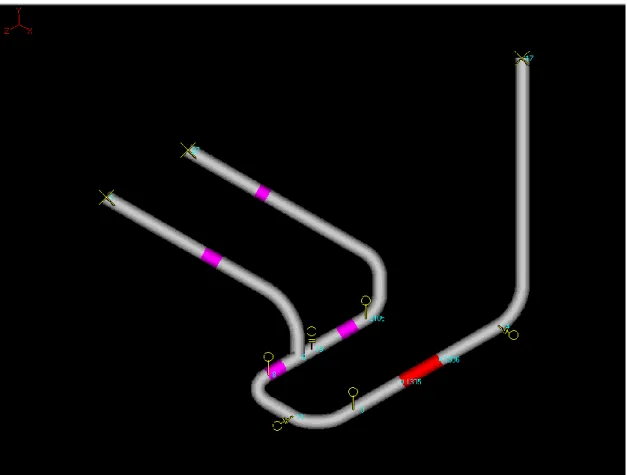
A model pipe system is developed for the analysis of environmental effects. The model system contains several of typical piping components such as elbows and tee junctions and should be fairly realistic.
The diameter D and the thickness t is the same for the whole system, D = 323.9 mm and t = 17.5 mm. The internal pressure is 7 MPa at all time and two different materials are tested; austenitic steel, 1.4306 and ferritic steel, 15Mo3. The pipe system is presented in Figure A1.
A2.2. Load cases
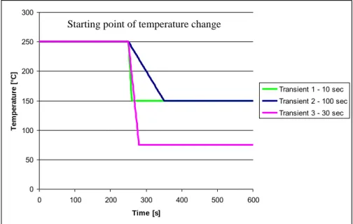
Three different transients are defined and applied to the model pipe system. The transients are chosen to have different characteristics in terms of strain rate and temperature. Transient 1 and 3 is rapid whereas transient 2 is con-siderably slower. Moreover, transient 3 covers a larger temperature range and thus passes over the temperature threshold at 150 oC. The transients are illustrated in Figure A2:.
0 50 100 150 200 250 300 0 100 200 300 400 500 600 Time [s] Te m pe ra ture [ °C ] Transient 1 - 10 sec Transient 2 - 100 sec Transient 3 - 30 sec
Figure A2: Three different transients that are applied at the pipe system
Transient 1: Temperature drops from 250°C to 150°C in 10 seconds
Transient 2: Temperature drops from 250°C to 150°C in 100 seconds
Transient 3: Temperature drops from 250°C to 75°C in 30 se-conds
Since Pipestress needs transients to be combined in pairs and allow the com-parison for full fatigue cycles each transient is input in pairs, i. e. in full tem-perature cycles. This means that the temtem-perature change displayed in Figure A2 is first applied, thereafter the temperature is held at steady state for a longer time, and finally the temperature is returned to the originating tem-perature (by mirroring the temtem-perature change in Figure A2:). This is illus-trated for transient 2 in Figure A3, which shows the pipe response to the applied transient.
0,0 50,0 100,0 150,0 200,0 250,0 300,0 0 500 1000 1500 2000 2500 Tim e [s] T em p er at u re [ ˚C ]
Figure A3: Transient pair 2 - the temperature drops from 250 °C to 150 °C and then reversed.
The pressure is kept constant and will have no influence on environmental factors and stress ranges. All analyses are fully elastic.
A3. Environmental fatigue life
correction factor (F
en
)
A3.1. The Inspecta method of
compu-ting F
en
and the usage factor
according to NUREG/CR-6909
Appendix A in NUREG/CR-6909 /A3/ describes how to calculate Fen. For a
transient the nominal Fen is calculated for every time step in the transient. ) 734 . 0 exp( , TO
Fennom (austenitic) (A1)
The parameters T´, O´ and
are transformed temperature, strain rate, and dissolved oxygen, DO, defined as0 T if T ≤ 150˚C
150
/
175
T
T
if 150˚C < T < 325˚C 1 T if T > 325˚C281
.
0
O
all DO levels 0
if
> 0.4 %/s
/
0
.
4
ln
if 0.0004 ≤
≤ 0.4 %/s
0
.
0004
/
0
.
4
ln
if
< 0.0004 %/s. ) ' 101 . 0 632 . 0 exp( , S TO
Fennom (ferritic) (A2)
The parameters are dependent on dissolved oxygen content in the water, DO, the sulphur content in the steel, S, the temperature, T and the strain rate,
, defined as 015 0 ' . S if DO > 1.0 ppm 001 0 ' . S if DO ≤ 1.0 ppm and S ≤ 0.001 wt.%S
S
'
if DO ≤ 1.0 ppm and 0.001 < S ≤ 0.015 wt.% 015 0 ' . S if DO ≤ 1.0 ppm and S > 0.15 wt.%0
'
T
if T ≤ 150˚C150
'
T
T
if 150˚C < T < 350˚C0
'
O
if DO ≤ 0.04 ppm
/
0
.
04
ln
'DO
O
if 0.04 ppm < DO ≤ 0.5 ppm
0
'
if
> 1%/s
'
ln
if 0.001 ≤
≤ 1%/s
0
.
001
ln
'
if
< 0.001 %/s.The modified rate approach /A3/ for calculating Fen is assumed to be the
most accurate method in that it integrates over each time in the transient and thus takes instant temperatures and strain rates into account.
n k k k k k en enF
T
F
1 max min ,(
,
)
(A3)It is a prerequisite for environmental effects to be active that the strain rate is positive. Negative strain rate is assumed to give no contribution to the envi-ronmental effects.
The expression in equation (A3) is then integrated over the strain and a unique value of Fen is obtained for each stress cycle. These values then give
a representative value of Fen for the transients to enable a direct comparison
with Pipestress. The method has a threshold value that is defined for a stress amplitude, the limit is 195 MPa for Austenitic steel and 145 MPa for Ferrit-ic. Below that value the Fen factor will result as 1.
A more precise description of the detailed method is found in previous works by Inspecta, ref. /A4/. A procedure for the detailed method was im-plemented by Inspecta. The environmental factor Fen is then computed in a
stand-alone procedure intended for the environmental factor only. The stress amplitudes are also computed but not intended for design, only for compari-son. In this method the influence of the type of component is considered by applying an appropriate stress raise factor, K to the total stress
range/amplitude. This factor is generally set to the same as the factor K3 in
equation (A5) below. The computed stress amplitudes will be given for comparison.
A3.2. The method of computing F
en
and the usage factor according
to Pipestress
DST has implemented the requirements of US NRC Regulatory Guide 1.207 /A5/ in version 3.6.2 of the program Pipestress /A1/.
Constant values for Fen are used in Pipestress through the entire transient.
These values are either user provided or default. The stepwise integration in equation (A3) is not used with Pipestress. Instead, the transformed tempera-ture, strain rate, dissolved oxygen and sulfur content are all held constant over the full transient. Thus, the user has to set appropriate values for each case or use the in-built default values for some of the constants. The default
values correspond to the most conservative settings possible, i. e. those that give a high Fen as possible.
For the temperature, DST recommends using the average temperature over the load set, the maximum value is considered to be too conservative. An important observation is that Pipestress will use the same Fen over the
entire piping system, unless the user provides differentiated parameters for each location.
In the present study, four different Pipestress analyses are performed for each transient, with different parameter value combinations for the strain rate and temperature. For the temperature, the average and maximum tempera-ture will be used.
Fen will be computed with two different strain parameter values. The default
strain rate in Pipestress represents lower bound strain rates. The other pa-rameter is represented by the average strain rate, which is calculated manual-ly. The average strain rate input is calculated in a simple way based on nom-inal transient times and stress range. This simple way is used since it re-quires no detailed modeling of strain rates, which is assumed to be the usual case for a common design situation. Mathematically, the mean strain rate is computed by simply dividing the elastic stress range with the nominal transi-ent time. This will provide an estimate of the average tensile strain rate, see Table A1.
.
Figure A4: Figure illustrating how the average tensile strain rate is derived. The stress range is divided by the time, T.
The parameters used in the study are shown in Tables A1-A3. Notably, Ta-ble A1 contains those parameters that are varied in order to investigate the results dependency on these parameters.
E MAX average /
(A4) 6 Transient 1 Transient 2 Str ai ns T T =E(max-min)Tensile
In this case the transient time, T, will be 10, 100 and 30 seconds for transient 1,2 and 3 respectively.
Table A1: Parameter set up combination for Pipestress
Pipestress parame-ter set-up
combina-tion
Strain rate Temperature
DO (Ferritic material
only)
S
(Ferritic material only) A
(def st, mean T)
0,0004%/s (Default)
Mean, see
Table A2-A3 0.4 ppm (Default) 0.015 weight % (Default)
B (var st, mean T)
Transient average, see Table A2-A3
Mean, see Table A2-A3 0.4 ppm (Default) 0.015 weight % (Default) C (def st, max T) 0,0004%/s (Default)
250 °C (Max) 0.4 ppm (Default) 0.015 weight % (Default)
D (var st, max T)
Transient average, see Table A2-A3
250 °C (Max) 0.4 ppm (Default) 0.015 weight % (Default)
Table A2: Complementary Pipestress values for Austenitic steel
Straight pipe Tee joint Elbow
Transient 1 2 3 1 2 3 1 2 3 Mean temperature [°C] 200 200 162.5 200 200 162.5 200 200 162.5 Stress amplitudes [MPa] 305 95 1) 385 462 1551) 620 729 254 1006 Strain rate [%/s] 0,016 0,0005 0,007 0,025 0,0008 0,01 0,04 0,0014 0,018
1) Below the threshold value for environmental effects in austenitic steels
Table A3: Complementary Pipestress values for Ferritic steel
Straight pipe Tee joint Elbow
Transient 1 2 3 1 2 3 1 2 3 Mean temperature [°C] 200 200 162.5 200 200 162.5 200 200 162.5 Stress amplitudes [MPa] 185 321) 179 296 531) 292 478 861) 477 Strain rate [%/s] 0,01 0,0002 0,003 0,016 0,0003 0,005 0,025 0,0005 0,008
A4. Data
The material data used in the calculations are shown below.
Table A4:Data for the Austenitic 1.4306 steel at 200 °C
E
[MPa] 185·103
[-] 0.29
[1/°C] 15·10-6
[W/m
oC]
17
[kg/m3] 7900 vC
[J/kg
oC]
525 h, [W/m2°C] 15000Table A5:Data for the Ferritic 15Mo3 steel at 200 °C
E [MPa] 189·103
[-] 0.30
[1/°C] 13·10-6
[W/m
oC]
47
[kg/m3] 7800 vC
[J/kg
oC]
533 h, [W/m2°C] 11500A5. Result
The detailed analysis can be regarded as the target analysis for the piping system shown in Figure A5. For Pipestress results to be acceptable they should not deviate too much from those produced by the detailed model. In the ideal situation, Pipestress, employing the more approximate method, should provide results that are somewhat conservative in comparison to the detailed method. However, taken the large uncertainty regarding the com-plex phenomenon of environmental effects the relative un-conservatism should certainly be accepted. A sensitivity analysis was performed for two parameters that have the most influences on the Fen value; the transformed
stain rate and temperature. Also a comparison for different local stress indi-ces has been evaluated. In equation 11 in ASME /A6/ for the peak stress intensity range, see equation (A5), the K values are the local stress indices.
2 3 3 3 1 3 0 2 2 0 0 1 1
1
1
)
1
(
2
1
2
2
T
E
K
T
T
E
C
K
T
E
K
M
I
D
C
K
t
D
P
C
K
S
b b a a ab i p
(A5)The value of K3 has the most influence on the stress range since the
tempera-ture stresses are highest. A closer look is done at three different locations on the pipe structure where a different value for the K3 factor is applied from
Pipestress. The results from Pipestress are compared with numerical calcula-tions performed with the NUREG/CR-6909 /A3/ method by Inspecta, named detailed method below.
elbow
junction
Straight pipe
Results for the austenitic piping are shown in the Tables A6-A8. A direct comparison between Pipestress computed Fen and detailed values is hence
enabled.
Table A6: Austenitic - 1.4306. Fenvalues for a straight pipe (K3=1
)
PIPESTRESS Detailed method A (def st, mean T) B (ave st, mean T) C (def st, max T) D (ave st, max T) Trans. 1 (10 s) 3.63 2.69 6.32 3.48 3.72 Trans. 2 (100 s) 1 1 1 1 1 Trans. 3 (30 s) 2.39 2.26 6.32 4.00 3.49Table A7: Austenitic - 1.4306. Fen values at a tee junction (K3=1.87)
PIPESTRESS Detailed method A (def st, mean T) B (ave st, mean T) C (def st, max T) D (ave st, max T) Trans. 1 (10 s) 3.63 2.60 6.32 3.25 3.46 Trans. 2 (100 s) 1 1 1 1 1 Trans. 3 (30 s) 2.39 2.24 6.32 3.70 3.27
Table A8: Austenitic - 1.4306. Fen values for an elbow (K3=3.3)
PIPESTRESS Detailed method A (def st, mean T) B (ave st, mean T) C (def st, max T) D (ave st, max T) Trans. 1 (10 s) 3.63 2.51 6.32 3.02 3.23 Trans. 2 (100 s) 3.63 3.29 6.32 5.18 4.36 Trans. 3 (30 s) 2.39 2.22 6.32 3.42 3.09
The results for the austenitic piping are further summarized in Figure A6. It is shown that combination D, i. e. average strain rate and maximum tempera-ture give overall very good results. This conclusion holds well regardless of transient and component for the austenitic material. Combination C, i. e. minimum strain rate and maximum temperature are well on the conservative side for all cases.
Figure A6: Summary of the results in tables A6 - A8. Pipestress provided Fen values compared to the detailed values.
The influence of the type of component in the austenitic piping is further analyzed with the detailed method. These results are presented in Table A9 and Table A10. Table A10 shows the Fen value relative to the straight pipe Fen. The results show that the influence of the type of component is small for
the austenitic piping.
Table A9: Austenitic - 1.4306. Fen values by the detailed method
Straight pipe K3=1 Tee K3=1.87 Elbow K3=3.3 Trans. 1 (10 s) 3.72 3.46 3.23 Trans. 2 (100 s) 1 1 4.36 Trans. 3 (30 s) 3.49 3.27 3.09
Austenitic - 1.4306
0 0.5 1 1.5 2 2.5 1 2 3 4 5 6 7 8 9 A (def st, mean T) B (ave st, mean T) C (def st, max T) D (ave st, max T)Straight Pipe Tee Elbow
1 2 3 1 2 3 1 2 3 TRANSIENT
Table A10: Austenitic - 1.4306. The influence of the K3 factor is compared for the Fen value
Table A11 is provided as an additional check of computed stress ranges for the austenitic piping. Pipestress and the detailed method are shown to pro-vide similar stress ranges.
Table A11: Austenitic - 1.4306. Stress comparison
Straight Pipe K3=1 Tee joint K3=1.87 Elbow K3=3.3
Transient 1 2 3 1 2 3 1 2 3 Stress amplitude (MPa) 305 95 385 462 155 620 729 254 1006 Stress amplitude – det. Meth (MPa)
247 94 350 459 178 644 807 317 1136
Difference 1.23 1.01 1.10 1.01 0.87 0.96 0.90 0.80 0.89
Results for the ferritic piping are given in Tables A12-A14.
Table A12:Ferritic – 15Mo3. Fen values for a straight pipe (K3=1)
PIPESTRESS Detailed method A (def st, mean T) B (ave st, mean T) C (def st, max T) D (ave st, max T) Trans. 1 (10 s) 6.28 4.22 20.94 9.45 9.17 Trans. 2 (100 s) 1 1 1 1 1 Trans. 3 (30 s) 2.54 2.42 20.94 14.03 9.05
Table A13: Ferritic – 15Mo3. Fen values for a tee junction (K3=1.87)
PIPESTRESS Detailed method A (def st, mean T) B (ave st, mean T) C (def st, max T) D (ave st, max T) Trans. 1 (10 s) 6.28 3.88 20.94 8.02 7.93 Trans. 2 (100 s) 1 1 1 1 1 Trans. 3 (30 s) 2.54 2.37 20.94 11.83 7.83 Straight pipe Tee Elbow
Trans. 1 (10 s) 1.00 0.93 0.87 Trans. 2 (100 s) -- -- 0.86 Trans. 3 (30 s) 1.00 0.93 0.88
Table A14: Ferritic – 15Mo3. Fen values for an elbow (K3=3.3)
A comparison between Tables A9-A11 and Tables A12-A14 shows that the environmental factors are higher for the ferritic piping than for austenitic piping. The value of Fen is higher for the ferritic piping by a factor ranging
from 2.1 to 2.6. The results for the ferritic piping are summarized in Figure A7. The Pipestress results relative to the detailed method are shown. It is shown that combination D, i. e. average strain rate and maximum tempera-ture give overall fairly good results. This conclusion holds well regardless of transient and component for the ferritic material. Combination C, i. e. mini-mum strain rate and maximini-mum temperature are well on the conservative side for all cases.
Figure A7: Summary of the results in tables A9 – A11. Pipestress provided en values compared to the detailed values.
PIPESTRESS Detailed method A (def st, mean T) B (ave st, mean T) C (def st, max T) D (ave st, max T) Trans. 1 (10 s) 6.28 3.57 20.94 6.79 6.88 Trans. 2 (100 s) 1 1 1 1 1 Trans. 3 (30 s) 2.54 2.32 20.94 9.96 6.82
Straight Pipe Tee Elbow
COMPONENT
Ferritic – 15Mo3
0 0.5 1 1.5 2 2.5 3 3.5 1 2 3 4 5 6 7 8 9 A (def st, mean T B (ave st, mean T) C (def st, max T) D (ave st, max T) 1 2 3 1 2 3 1 2 3 TRANSIENTThe influence of the type of component is further analyzed with the detailed method. These results are presented in Table A15 and Table A16. Table A16 shows the Fen value relative to the straight pipe Fen, which is the highest
val-ue for all cases. The results show that the inflval-uence of the type of component is fairly small for the ferritic piping also.
Table A15: Ferritic – 15Mo3. Fen values by the detailed method
Straight pipe K3=1 Tee K3=1.87 Elbow K3=3.3 Trans. 1 (10 s) 9.17 7.93 6.88 Trans. 2 (100 s) -- -- -- Trans. 3 (30 s) 9.05 7.83 6.82
Table A16: Ferritic – 15Mo3. The influence of the K3 factor is compared for the Fen value
Straight pipe Tee Elbow
Trans. 1 (10 s) 1.00 0.86 0.75
Trans. 2 (100 s) -- -- --
Trans. 3 (30 s) 1.00 0.86 0.76
Table A17 is provided as an additional check of computed stress ranges for the ferritic piping. Pipestress and the detailed method are shown to provide similar stress ranges.
Table A17: Ferritic – 15Mo3. Stress comparison
Straight Pipe K3=1 Tee joint K3=1.87 Elbow K3=3.3
Transient 1 2 3 1 2 3 1 2 3 Stress ampli-tude [MPa] 185 32 179 296 53 292 478 86 477 Stress ampli-tude – det. Meth [MPa] 156 36 167 290 64 314 510 113 555 Difference 1.19 0.86 1.07 1.02 0.83 0.93 0.94 0.76 0.86
A6. Conclusions
The implementation of a computational procedure for the environmental factor, Fen, in Pipestress has been investigated. The investigation has been
carried out by analysis with three transients on a model piping system. The Pipestress results were compared with results obtained by a detailed proce-dure developed by Inspecta Technology, based on the instructions in NU-REG/CR-6909 (the ANL-procedure). The comparisons were performed for austenitic and ferritic steels.
The implementation of the environmental factor computation in Pipestress is simple. No detailed integration with time varying parameters is per-formed. Instead all parameters remain constant throughout the transients.
The parameter values are given as default by Pipestress unless other values are provided by the analyst.
The comparison shows that these constant parameter values for Pipestress must be chosen with care in order to obtain results comparable to those ob-tained by the detailed calculations.
Calculations with mean transient temperature values as input should be avoided, since the environmental factors tend to become significantly low-er than the values dlow-erived by the detailed calculations. Instead maximum transient temperatures should be used as input.
If maximum temperatures are combined with average strain rates the cor-relation between Pipestress and the detailed method is surprisingly good. Clear conservatism in relation to the detailed methods is obtained if lower bound strain rates are used as input instead of mean values.
These model examples show the importance of the temperature values for the computed Fen values.
The strain rate is of less importance, however not negligible.
The local stress indices K3, raise the stress ranges up to three times the
value for a straight pipe. However, this only results in 15-30 % increase of the Fen value. Hence, the computed Fen is fairly independent of the
compo-nent type.
The environmental factors were larger for the ferritic steel piping than for the austenitic steel piping by a factor to the order of 2-2.5 for identical transients.
Pipestress with its current implementation for environmental factors should not be used as a research tool for environmental effects. However, Pipestress can be used as effective tool for considering environmental ef-fects in the engineering analysis of piping systems. It is recommended that the maximum transient temperature is always chosen for input.
A7. References
/A1/ Pipestress, DST, version 3.6.2
/A2/ Catalano, J., Specification for Implementation of US NRC R.G.
1-207 in Pipestress Computer Program Specification No. DST-spec-2008-1 Revision 1, DST Computer Services, S.A., July 2009.
/A3/ Chopra, O., K, Shack, W.,J., Effect of LWR Coolant Environments
on the Fatigue Life of Reactor Materials, NUREG/CR-6909,
ANL-06/08.
/A4/ Steingrimsdottir, K., Dahlberg, M., A fatigue analysis including
environmental effects for a pipe system in a Swedish BWR ,
Tech-nical report no. 50009450-4, Inspecta Tehnology AB, 2010. /A5/ U.S. Nuclear regulatory commission, Regulatory Guide 1.207,
Office of Nuclear Regulatory Research, March 2007.
/A6/ ASME Boiler & Pressure Vessel Code, ASME III, Division 1, NB-3000, 2007.
2011:30 The Swedish Radiation Safety Authority has a comprehensive responsibility to ensure that society is safe from the effects of radiation. The Authority works to achieve radiation safety in a number of areas: nuclear power, medical care as well as commercial products and services. The Authority also works to achieve protection from natural radiation and to increase the level of radiation safety internationally.
The Swedish Radiation Safety Authority works proactively and preventively to protect people and the environment from the harmful effects of radiation, now and in the future. The Authority issues regulations and supervises compliance, while also supporting research, providing training and information, and issuing advice. Often, activities involving radiation require licences issued by the Authority. The Swedish Radiation Safety Authority maintains emergency preparedness around the clock with the aim of limiting the aftermath of radiation accidents and the unintentional spreading of radioactive substances. The Authority participates in international co-operation in order to promote radiation safety and fi nances projects aiming to raise the level of radiation safety in certain Eastern European countries.
The Authority reports to the Ministry of the Environment and has around 270 employees with competencies in the fi elds of engineering, natural and behavioural sciences, law, economics and communications. We have received quality, environmental and working environment certifi cation.