Handling Interfaces and Time-varying
Properties in Radionuclide
Transport Models
2011:11
Authors: Peter RobinsonClaire Watson
SSM perspective
Background
The application for a KBS-3 type spent nuclear fuel repository will be supported by a post-closure safety assessment (SR-Site) which includes modelling of radionuclide transport from an underground source term. In order to prepare for the review of the oncoming license application the Swedish Radiation Safety Authority (SSM) has performed research and development projects in the area of performance assessment mo-delling during recent years. Independent momo-delling capability has been established, both at SSM and with external consultants. This has included the development of approaches and models for consequence analysis (radionuclide transport) that can be used to support the review of a spent nuclear fuel repository.
Objectives
In this project the following three areas were investigated:
1. The Qeq concept is an important part of SKB’s current methodo-logy to model transport resistance at the buffer/fracture interface for radionuclide transport. The regulatory review of SKB’s earlier safety analysis shows that the transport resistance offered by the buffer/fracture interface is a critical component for radionuclide transport. The Qeq concept is reviewed and calculations under-taken to explore whether this remains valid in situations where heterogeneity or spalling are present.
2. Some assessment calculations are undertaken to investigate the potential for changes in transport properties with time due to the effects of glacial episodes that could affect radionuclide transport to the surface.
3. SKB has developed a new code MARFA for handling spatially varying properties and time-varying flows relating to radionuclide transport problems for the far field. This code may be used in parallel with the older geosphere transport approach (FARF31) in SR-Site, therefore, the code is reviewed and analysed by Quintessa’s independent model.
Results
Quintessa’s QPAC code has been used to investigate the Qeq approach. The conclusions from this simulation study are the following. The basic approach to calculating Qeq values is sound, however, narrow channels could lead to the same release as larger fractures with the same pore velocity, so a channel enhancement factor of √10 should be considered. A spalling zone that increases the area of contact between flowing water and the buffer has the potential to increase the release significantly. Quintessa’s AMBER software has been used to explore the effects of glacial episodes on radionuclide transport with time-varying properties. The simulation results show that for both single and multiple glacial episodes the time-dependency of model parameters did not result in
much change to the calculated peak fluxes to the biosphere. These con-clusions are preliminary and could be changed if different radionuclides are important in the SR-Site assessment.
A detailed review of MARFA code and the associated documentation has been undertaken. New semi-analytic methods have been developed in order to provide a means of checking the accuracy of MARFA calculations. The strengths and weaknesses of MARFA code have been explored in detail.
Project information
Project manager: Shulan Xu Project reference: SSM 2010/829
2011:11
Authors: Peter Robinson and Claire Watson Quintessa Ltd. UK
Handling Interfaces and Time-varying
Properties in Radionuclide
This report concerns a study which has been conducted for the Swedish Radiation Safety Authority, SSM. The conclusions and view-points presented in the report are those of the author/authors and
Summary
This report documents studies undertaken by Quintessa during 2010 in preparation for the SR-Site review that will be initiated by SSM in 2011. The studies relate to consequence analysis calculations, that is to the calculation of radionuclide release and transport if a canister is breached. A sister report documents modelling work undertaken to investigate the coupled processes relevant to copper corrosion and buffer erosion.
The Qeq concept is an important part of SKB’s current methodology for radionuclide transport using one-dimensional transport modelling; it is used in particular to model transport at the buffer/fracture interface. Quintessa’s QPAC code has been used to investigate the Qeq approach and to explore the importance of heterogeneity in the fracture and spalling on the deposition hole surface. The key conclusions are that:
The basic approach to calculating Qeq values is sound and can be reproduced in QPAC.
The fracture resistance dominates over the diffusive resistance in the buffer except for the highest velocity cases.
Heterogeneity in the fracture, in terms of uncorrelated random variations in the fracture aperture, tends to reduce releases, so the use of a constant average aperture approach is conservative.
Narrow channels could lead to the same release as larger fractures with the same pore velocity, so a channel enhancement factor of
10
should be considered. A spalling zone that increases the area of contact between flowing water and the buffer has the potential to increase the release significantly and changes the functional dependence of
Q
eqfrac on the flowing velocity. Quintessa’s AMBER software has previously been used to reproduce SKB’s one-dimensional transport calculations and AMBER allows the use of time-varying properties. This capability has been used to investigate the effects of glacial episodes on radionuclide transport. The main parameters that could be affected are sorption coefficients and flow rates. For both single and multiple glacial episodes the time-dependency of model parameters did not result in much change to the calculated peak fluxes to the biosphere. This is because fluxes are calculated to be dominated by the poorly-sorbed radionuclides 129I and 36Cl. However, a small increase (less than an order of magnitude) in the overall flux contributed from the radium decay chain, which is important for long timescales, was calculated during the phase when the multiple glacial episodes are occurring. These conclusions arepreliminary and could be changed if different radionuclides are important in the SR-Site assessment.
The known shortcomings of its one-dimensional radionuclide transport modelling capability has led SKB to fund the development of the MARFA code, which it is understood will be used in addition to the existing methodology in SR-Site. A detailed review of this code and the associated documentation has been undertaken. New semi-analytic methods have been developed in order to provide a means of checking the accuracy of MARFA calculations. The key conclusions are that:
MARFA can handle large networks in practicable run times, generally works well for single radionuclides or short chains and accurately handles advective systems where matrix diffusion effects are dominant.
The code has, however, a number of important limitations. In particular, it is unable to handle long decay chains with short-lived radionuclides and calculations immediately after flow rate changes can be inaccurate.
The documentation and Quality Assurance are poor. A large number of errors have been found in the User Guide and the associated test cases do not adequately test the use of the code for the anticipated applications.
These limitations bring into question the code’s suitability (in its
present form) for performance assessment calculations for a deep radioactive waste repository.
Content
1 Introduction 1
2 The Fracture-buffer Interface 2
2.1 Qeq Formulae 2 2.2 Modelling Approach 4 2.3 Reference Calculations 9 2.4 Fracture Heterogeneity 13 2.5 Spalling 15 2.6 Conclusions 16
3 Time-dependence in Radionuclide Transport Calculations 18
3.1 Background 18
3.2 Conceptual Model 18
3.3 Calculations 26
3.4 Conclusions 31
4 Review and Testing of MARFA 32
4.1 General Overview 33 4.2 Documentation 34 4.3 The Code 35 4.4 Algorithms 39 4.5 Documented Tests 47 4.6 Additional Tests 56 4.7 MARFA 3.3 63 4.8 Conclusions 64 5 Overall Conclusions 66 References 68 Appendix A: Nomenclature 71 Appendix B: Semi-analytic Solutions for Radionuclide Transport
1 Introduction
This report documents studies undertaken during 2010 in preparation for the SR-Site review.
The studies described here relate to consequence analysis calculations, that is to the calculation of radionuclide release and transport if a canister is breached. A sister report [1] documents modelling work undertaken to look at the coupled issues of copper corrosion and buffer erosion.
The studies into some aspects of consequence analysis follow on from work in previous years ([2] and [3]). The objective of this work is to prepare for review of SR-Site by developing an understanding of the key issues and of SKB’s assessment approach.
In this year’s work, three aspects were examined.
The first area studied is the important interface between the buffer and a flowing fracture. SKB’s use of the Qeq concept is reviewed and calculations undertaken to explore whether this remains valid in situations where heterogeneity or spalling are present. This is documented in Section 2.
Secondly, some assessment calculations have been undertaken to investigate the potential for changes in transport properties with time to affect radionuclide transport to the surface. In particular, the importance of near-surface geochemical changes is considered and documented in Section 3.
Finally, the MARFA code is reviewed in some detail. This code may be used in parallel with the older geosphere transport approach (FARF31) and it is important to understand its strengths and weaknesses. The review is documented in Section 4 and additional mathematical details are given in Appendix B.
2 The Fracture-buffer
Interface
Radionuclides released from a breached canister while the buffer remains intact will move through the buffer by diffusion. In order to enter the geosphere and ultimately reach the surface, they must enter flowing water. Several possible routes have been identified [4], and release to a fracture that intersects the deposition hole is an important route.
Release through this route is constrained by the nature of the interface between the buffer and the fracture. First, the fracture has a small aperture and diffusion to the small area that this implies is limited. Second, the entry of radionuclides into the flowing fracture water requires that they diffuse away from the interface.
SKB developed an approach to handling transport across this interface [5] which has been used in subsequent assessments and which can be expected to be used in SR-Site. This leads to the specification of an equivalent flow,
Qeq, at the interface. A review of the approach employed was reported in [6] where the derivations were found to be correct but concern was expressed that the application of the formulae in probabilistic cases needed to be handled carefully. In SR-Can, the potential for spalling was recognised and an adjustment was made to Qeq to allow for this. This was reviewed in [2] and found to be provisional and speculative and not clearly documented. The approach is described as conservative in [7].
The SKB approach uses an idealised geometry. In particular, the fracture is open with a constant aperture. In reality, it is thought that fractures will have highly variable apertures and may be channelled. For the main geosphere transport calculations in SR-Can, SKB applied a channelling factor of 10 to the F-factors calculated in their flow models (implying that flow is largely confined to 10% of the fracture area), but no similar modification was discussed in relation to the fracture-buffer interface.
The purpose of the current study is to confirm that the basic Qeq approach is sound and to explore the impacts of heterogeneity in the fracture and spalling on the deposition hole surface.
2.1 Q
eqFormulae
The Qeqapproach to transport across interfaces can be explained as follows. Given a steady driving concentration (for example at the canister surface),
0
(e.g. the buffer and the fracture near the deposition hole) is
(mol y-1) then this is equivalent to a flow rate Qeq (m3 y-1) where0 C Qeq
. (2.1.1)
Where there are two sections in sequence, an overall
Q
eqcan be calculated to be given by ) 2 ( ) 1 (1
1
1
eq eq eqQ
Q
Q
. (2.1.2)This is clear if
Q
eqis thought of as a conductance with its reciprocal being a resistance.For the specific case of interest, the two components are the resistance on the buffer side and the resistance on the fracture side. Writing the interface concentration as
C
int, with the concentration in the fracture far from thedeposition hole being zero, we write
int int 0 0
Q
(
C
C
)
Q
C
C
Q
eq
eqbuff
eqfrac
, (2.1.3)From which it is easy to derive the reciprocal relationship between the various Qeqvalues: frac eq buff eq eq
Q
Q
Q
1
1
1
. (2.1.4)It is also clear from physical considerations that the smaller of the eq
Q component values determines the overall value and that the interface concentration will be closer to the concentration on the side with the largerQeq.
A detailed discussion was given in [6]; here we note the final results.
For the buffer
b F RD Qeqbuff eff / 4
(2.1.5)where R is the distance from the canister to the fracture and F/b is calculated from a regression fit as
b
a
R
a
b
F
/
0
.
9
1
.
466
log
10/
1
.
58
log
10/
(2.1.6) where a is half the relevant height of the canister where the concentration is fixed. The relevant height might be for a physical area where there is a breach in the canister, or simply half the distance between two fractures, where it represents the zone that would feed into a particular fracture.For the fracture,
Lv
D
b
Q
frac w eq
1
6
(2.1.7)where
D
wis the pore-water diffusion coefficient for the fracture water (equal to the effective diffusion coefficient since the fracture is assume to be open),L is the contact distance between the flowing water and the buffer, b is half
the fracture aperture and v is pore-water velocity. Note that a factor of 2 has been added to this formula to account for the full fracture aperture.
Various geometrical approximations are made in deriving these results.
For the buffer, it is assumed that the same concentration applies all around the interface, which is clearly not the case as there is a particular flow direction that will lead to different upstream and downstream concentrations. Also, the radial geometry is ignored – in [7] it is stated that this leads to about a 5% error. The main effect is that the circumference of the canister is treated as if it were the same as the outer buffer circumference, so it is likely that this overstates the Qeq and so is conservative. The analysis was also undertaken for a set of identical fractures, so that symmetry conditions could be imposed.
For the fracture, the key approximation is that the interface is taken to be linear in Cartesian coordinates with a constant flow velocity past it. In fact, of course, it is cylindrical and the flow will vary significantly along its length (the fastest flow being half way around between the upstream and downstream directions).
Our objective is to check that these approximations do not give significantly incorrect values forQeq.
2.2 Modelling Approach
The approach used here is to model the deposition holes and a fracture that intersects it numerically. The QPAC software [8] was used, modelling Darcy flow (in the fracture) and tracer transport (advection and diffusion of a marker species) in the buffer and fracture.
In order to reduce the size of the model, a symmetry plane was used along the direction of flow. A unit concentration is imposed on a band of the
canister, extending above and below the fracture plane. This might represent a region where a breach has occurred, and so matches one of the interpretations of the “a” parameter given above. All other concentration are then relative to this.
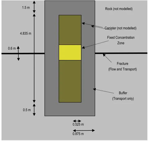
The physical dimensions and layout are illustrated in Figure 1.
Figure 1: Schematic cross-section through the modelled region, showing the key features and dimensions
Because the interface is narrow, it is important to have sufficient grid cells near it. Convergence tests were run and a grid was selected which gave results that changed by less than 1% compared to a grid with half the number of cells.
The grid is defined in cylindrical coordinates as a series of uniform or geometric sections in each coordinate. Table 1 and Table 2 give the azimuthal and radial grid sizes respectively. In the angular direction, 18 cells are used each with an angle of 10 degrees.
The buffer and fracture were treated as separate subsystems, with a Joiner subsystem connecting them and providing the required continuity of concentrations and fluxes.
0.525 m 0.875 m 0.5 m
4.835 m
1.5 m Rock (not modelled)
Canister (not modelled)
Fracture (Flow and Transport)
Buffer (Transport only) Fixed Concentration
Zone 0.6 m
Table 1 Grid cell sizes in the z direction
From To Type Number
Bottom of buffer Bottom of Can Uniform 3
Bottom of Can Bottom of Fixed
Concentration Zone Uniform 4 Bottom of Fixed Concentration Zone Bottom of Fracture Plane
Geometric 12, with last equal to fracture aperture Bottom of Fracture Plane Top of Fracture Plane 1 Top of Fracture Plane Top of Fixed Concentration Zone Geometric 12 Top of Fixed Concentration Zone
Top of Can Uniform 4
Top of Can Top of Buffer Uniform 3
Table 2 Grid cell sizes in the r direction
From To Type Number
Centre axis Can radius Uniform 3
Can radius Buffer Radius Geometric 15, with last equal to half
fracture aperture Buffer Radius Near buffer radius
(0.9 m)
Geometric 10, with first equal to fracture aperture Near buffer radius Edge of model
(10 m)
Geometric 10, with first equal to 2 cm
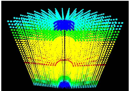
Because of the small size of many of the cells, it is hard to visualise the grid in spatial coordinates. Instead, Figure 2 shows the grid in “index coordinates”, i.e. each cell is treated as having the same size. The zones are colour coded to show how they correspond to the real geometry. The view is from above, looking down at an angle. Figure 3 shows the buffer grid in spatial coordinates, noting that the cell boundaries are not all visible in this figure.
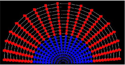
Figure 4 and Figure 5 show the fracture grid in the same ways. Note that the interfaces are shown in Figure 5 – these were hidden for the buffer grid. The near buffer zone is used for the heterogeneity tests.
Figure 2: The buffer grid showing the different zones in index coordinates
Figure 3: The buffer grid showing the different zones in spatial coordinates
Figure 4: The fracture grid showing the different zones in index coordinates
Figure 5: The fracture grid showing the different zones in spatial coordinates
The calculation of Qeqonly requires a steady state calculation. QPAC can calculate this directly. Given that results are required for a range of velocities, it is convenient to impose a time-dependent velocity and so calculate a sequence of results in a single QPAC run.
In order to calculate the individual
Q
eqbuffandQ
eqfracvalues, it is necessary to define a single interface concentration. The joiner subsystem calculates an interface concentration for each interface between a fracture and a buffer cell. We take a simple arithmetic average of these, on the basis that they all have similar areas and the concentration variation is small.2.3 Reference Calculations
The first set of calculations is aimed at a direct comparison with the Qeq
formulae used by SKB. Geometric properties are as in Figure 1. An aperture of 0.1 mm was used initially, with pore velocities ranging from 0.1 to 10 000 m/y. Other transport properties are given in Table 3
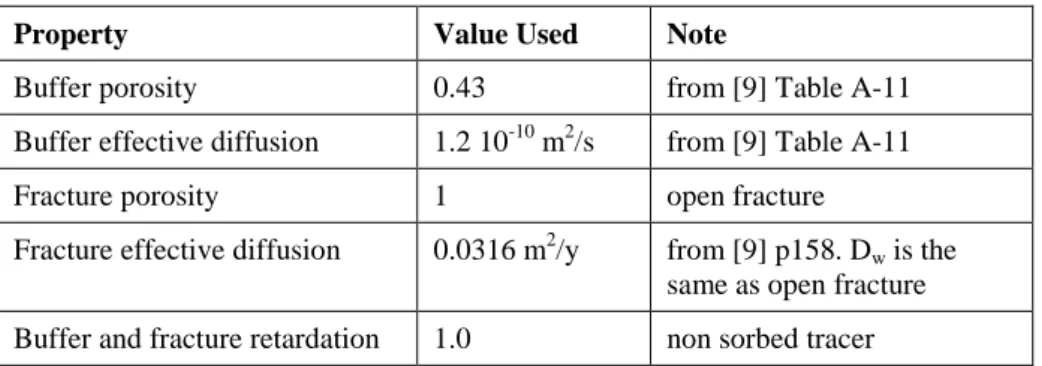
Table 3 Reference transport properties
Property Value Used Note
Buffer porosity 0.43 from [9] Table A-11
Buffer effective diffusion 1.2 10-10 m2/s from [9] Table A-11
Fracture porosity 1 open fracture
Fracture effective diffusion 0.0316 m2/y from [9] p158. Dw is the
same as open fracture
Buffer and fracture retardation 1.0 non sorbed tracer
The
Q
eqbuff value should be essentially independent of the flow velocity, as it depends only on the buffer properties. In practice there might be a small variation, because of the variation of concentrations at the interface for example.In fact, the numerically calculated value does not change across the whole velocity range. A value for
Q
eqbuffof 5.56e-3 m3/y is obtained. This compares to a formula (equation 2.1.5) value of 6.36e-3 m3/y. Thus, there is a 15% difference on the conservative side, which is a little larger than claimed in [10].We note that experiments while assessing grid convergence showed that the buffer beyond the immediate vicinity of the fracture has a rather small influence. Inappropriate gridding near the fracture can lead to significant errors (factors of two or more).
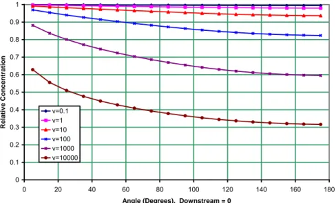
Figure 6 shows the concentration profile around the interface (at several velocities). There are two points to note here. First, the concentration is close to unity (recall that the canister concentration is unity) except for the very highest velocities, indicating that the buffer is not dominating the release. Second, the variation around the circumference is significant and so the fact that the calculated
Q
eqbuffis constant suggests that the local flux scales with the local concentration all around the circumference.Figure 7 shows the overall pattern of concentrations in the fracture for a central case. There is a clear upstream-downstream difference as expected. The lower velocity cases show less differences between upstream and
downstream but the concentrations are higher throughout. The highest flow case has a small plume downstream only.
0 0.1 0.2 0.3 0.4 0.5 0.6 0.7 0.8 0.9 1 0 20 40 60 80 100 120 140 160 180
Angle (Degrees). Downstream = 0
R el ati ve C o n cen tr ati o n v=0.1 v=1 v=10 v=100 v=1000 v=10000
Figure 6: Concentrations around the fracture-buffer interface for a range of velocities
Figure 7: Concentrations in the fracture for the 100 m/y flow case, in index coordinates
The
Q
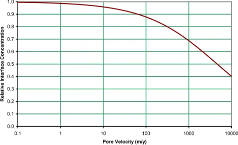
eqfrac values should depend on the flow velocity. Figure 8 shows the numerically calculated and formula values (equation 2.1.7). It is clear that there only a small discrepancy (16% at low velocities and 24% at high velocities). The values are much lower than for the buffer except for the largest velocities. Figure 9 shows the average concentration on the interface. The buffer and fracture components become equal when the average concentration reaches 0.5.1.E-05 1.E-04 1.E-03 1.E-02 1.E-01 0.1 1 10 100 1000 10000
Pore Velocity (m/y)
Qeq (m 3/y) QeqFrac Formula QeqFrac Calculated QeqBuff Calculated
Figure 8: Comparison of calculated and formula values of Qeq
across a range of velocities
0.0 0.1 0.2 0.3 0.4 0.5 0.6 0.7 0.8 0.9 1.0 0.1 1 10 100 1000 10000
Pore Velocity (m/y)
R el ati ve In ter face C o n cen tr ati o n
Figure 9: Average concentration on the fracture-buffer interface across a range of velocities
These calculations have been repeated for two other apertures: 0.3 mm and 1 mm. Figure 10 and Figure 11 show the results. The QPAC calculated
buff eq
Q
values are 6.22e-3 m3/y and 7.13e-3 m3/y, compared to formula values of 7.12e-3 m3/y and 8.20e-3 m3/y. These are both about 15% different on the conservative side, very similar to the 0.1 mm case.The
Q
eqfrac values show that the buffer and fracture components become equal at much lower velocities for the larger apertures. It is clear that there is only a small discrepancy (16% at low velocities and 24% at high velocities) of the same size as in the case with a fracture aperture of 0.1 mm.1.E-05 1.E-04 1.E-03 1.E-02 1.E-01 0.1 1 10 100 1000 10000
Pore Velocity (m/y)
Qeq (m 3/y) QeqFrac Formula QeqFrac Calculated QeqBuff Calculated
Figure 10: Comparison of calculated and formula values of Qeq
across a range of velocities for an aperture of 0.3 mm
1.E-05 1.E-04 1.E-03 1.E-02 1.E-01 0.1 1 10 100 1000 10000
Pore Velocity (m/y)
Qeq (m 3/y) QeqFrac Formula QeqFrac Calculated QeqBuff Calculated
Figure 11: Comparison of calculated and formula values of Qeq
across a range of velocities for an aperture of 1 mm
These results indicate that the Qeq formulae give a good approximation to the release in the simple planar geometry.
2.4 Fracture Heterogeneity
In order to treat heterogeneity in the fracture, we impose a varying porosity value. This is numerically simpler to handle than varying the aperture, where discontinuous cross-sectional areas would be hard to handle.
We start by taking a 0.2 mm aperture with a porosity of 0.5 throughout. This is expected to give similar results to the earlier calculations for a 0.1 mm open fracture and this is confirmed numerically – the
Q
eqfrac values agree to 4 significant figures.We now vary the porosity in a zone near to the buffer. The porosity further away is not varied because the grid cells are larger there and an average is more appropriate and because the impact is expected to come from the zone near to the fracture (as can be seen by the concentrations in Figure 7 for example). Conductivities are scaled with the square of the porosity, because it is intended that the porosity change should represent an aperture change and a Pouseille flow law can be assumed. The effective diffusion scales with porosity.
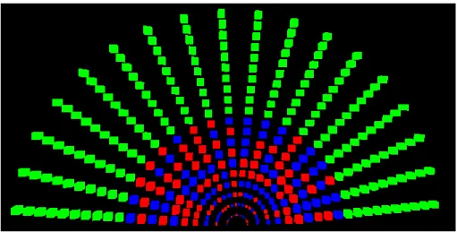
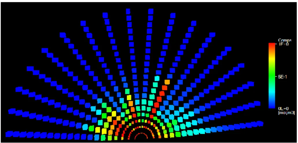
A randomly sampled porosity was used, with half the cells set to 0.01 and the other half to 0.99. Figure 12 shows the sampled porosity values. The concentrations for the 100 m/y velocity case are shown in Figure 13. The local impact of the porosity variations can clearly be seen.
Figure 12: Porosity values for the heterogeneity test. Red = 0.01, Blue = 0.99, Green = 0.5
Figure 13: Concentrations for the heterogeneity test for a velocity of 100 m/y
The effect obviously depends on the porosity samples. A second concentration calculation for a different sample is shown in Figure 14.
Figure 14: Concentrations for the heterogeneity test for a velocity of 100 m/y with a second sampled porosity field
The
Q
eqfrac calculations differ for each realisation. Figure 15 shows results for 8 such realisations, compared to the uniform case. It is clear that the heterogeneity reducesQ
eqfracand that the reduction depends both on the particular realisation and on the overall velocity. The velocity dependence depends on the details of the distribution of high and low porosities. It appears that at low velocities there is less sensitivity to the realisation than for the higher velocities. At low velocities there is up to a factor of two reduction from the uniform case; for intermediate velocities this increases to almost a factor 10 before reducing again. There is some indication that for very high velocities the factor again increases, but these are beyond the range of interest.1.E-05 1.E-04 1.E-03 1.E-02 1.E-01 0.1 1 10 100 1000 10000
Pore Velocity (m/y)
Qeq
(m
3/y)
QeqFrac Constant Porosity QeqBuff Calculated QeqFrac Varying Porosity 1 QeqFrac Varying Porosity 2 QeqFrac Varying Porosity 3 QeqFrac Varying Porosity 4 QeqFrac Varying Porosity 5 QeqFrac Varying Porosity 6 QeqFrac Varying Porosity 7 QeqFrac Varying Porosity 8
Figure 15: Comparison of calculated values of Qeq across a range of
velocities for constant and varying porosity fields
Overall, the effect of randomly varying porosity with no correlation structure (which can be interpreted as varying fracture aperture) is to reduce releases, so taking a constant fracture aperture is conservative.
The examples shown here did not have any correlation in the porosity choices and so did not include channels [11]. It is clear that the length scale over which the concentration falls away from the interface value is small (a few cm), so any channel of that size would act in the same way as a full fracture. Therefore, if there is a channelling factor of 10 (all the flow is in 10% of the fracture), it is clear that the effect can be the same as a 10 times larger velocity (giving a factor of
10
forQ
eqfrac).2.5 Spalling
In order to look at the effect of a localised spalling zone at the edge of the buffer, we introduce a zone of high conductivity in a zone above and below the fracture. The size of the zone is chosen for gridding convenience to be the same as the unit concentration zone on the canister. It extends a distance of 2.5 cm into the rock. Thus there is an enhanced area of contact between the flowing water and the buffer.
Figure 16 shows results for the spalling case. The
Q
eqbuff value in the spalling case is higher, as would be expected because of the much larger contact area, and varies with velocity to a small degree. More importantly,Q
eqfrac is much larger and appears to scale directly with velocity, rather than the square-root. This arises because the constriction at the interface has been removed and there is now advection from the spalling zone into the main part of thefracture. It is the advection at this interface that controls the release – hence the linear dependence.
1.E-05 1.E-04 1.E-03 1.E-02 1.E-01 1.E+00 0.1 1 10 100 1000 10000
Pore Velocity (m/y)
Qeq
(m
3/y)
QeqFrac no Spalling Zone QeqFrac with Spalling Zone QeqBuff no Spalling Zone QeqBuff with Spalling Zone
Figure 16: Comparison of calculated values of Qeq across a range of
velocities for the spalling case
Thus, the impact of spalling, even when it is localised, can be significant. This is an important area for review in SR-Site since the approach used in SR-Can was provisional.
There is a need to model the spalling zone in a more realistic way, but the calculations here show that simply increasing the contact area (without any significant extra flow) is significant.
2.6 Conclusions
The calculations presented here have shown that:
the basic approach to calculating Qeq values is sound and can be reproduced in a numerical model;
the fracture resistance dominates over the diffusive resistance in the buffer except for the highest velocity cases;
heterogeneity in the fracture, in terms of uncorrelated random variations in the fracture aperture, tends to reduce releases, so a constant average aperture approach is conservative;
length scales for the release are such that narrow channels would lead to the same release as larger fractures with the same pore velocity, so a channel enhancement factor of
10
should be considered; a spalling zone that increases the area of contact between flowing water and the buffer has the potential to increase the release significantly and changes the functional dependence of
Q
eqfrac on the flowing velocity.3 Time-dependence in
Radionuclide Transport
Calculations
3.1 Background
To date, SKB have used a one-dimensional transport modelling approach using the FARF31 code [12], [13]. As stated in the main SR-Can report [4], one limitation of the migration path concept is that only steady-state velocity fields can be addressed whereas clearly the flow field will evolve in time (due to factors such as shoreline displacement and glacial advance and retreat). These and other limitations led to the development of the MARFA code, reviewed in Section 4.
Quintessa’s AMBER software [14] has previously been used to reproduce SKB’s transport calculations (e.g., [2]). AMBER allows the use of time-varying properties although this has not previously been exploited in calculations undertaken by Quintessa for SKI or for SSM. Here this capability has been used to investigate the effects of glacial episodes on the radionuclide transport. The main parameters that could be affected are the sorption coefficients and flow rates. The capabilities of AMBER allow smooth transitions between parameter values for temperate, glacial advance/retreat and glacial completeness conditions, which is not possible with MARFA or the Quintessa semi-analytic approach described in Appendix B. We note that the QPAC code [8] could also have been used for these calculations, but that it was convenient to continue with the established AMBER model.
Here we focus on releases from the geosphere. The question of how to use these to calculate doses to humans is also important, but it is understood that the landscape dose factor (LDF) method used by SKB in SR-Can will be replaced in SR-Site. Therefore no dose calculations are presented in the current report, and results are shown in terms of fluxes.
3.2 Conceptual Model
3.2.1 Description
The calculations described here are based on the pinhole failure scenario considered by SKB in SR-Can [4]. Although new welding techniques may mean that the risk of pinhole failures in canister welds is negligible, this case is useful for examining the safety role that the buffer and host rock play in
the multi-barrier concept. It is also representative of other failure modes, e.g. canister corrosion.
A brief description of the pinhole failure scenario calculations is given here; full details can be found in the SR-Can reports [4], [9] and in [2]. As previously indicated, the SKB transport models employed for SR-Can did not include time-varying properties and therefore parameter values (such as those for sorption coefficients and flow rates) were employed that are suitable for temperate interglacial periods. In this study a base case calculation that adopts the same approach as SKB has been undertaken together with variant time-varying calculations that consider glacial cycles and allow parameters to vary accordingly.
In order to focus on the effects of time-varying properties, deterministic calculations have been employed here using best estimate parameter values. The calculations presented here consider only the Q1 pathway (a fracture intersecting the deposition hole) since, as discussed in [3], this helps to focus attention on the issues being addressed without the complicating factor of different transport pathways. A schematic illustration of the near field is shown in Figure.17.
The canister is assumed to have a pinhole defect from the start, but this does not become an open pathway due to water intrusion until 1000 years after repository closure. The defect eventually leads to failure of the canister after 10 000 years. The flux of radionuclides into the buffer is limited by their solubility in water.
Once radionuclides have entered the bentonite buffer, they are transported by diffusion. The buffer is assumed to remain intact throughout the simulation. Sorption onto the clay mineral surfaces is modelled using sorption coefficients (Kd).
As described above, the only pathway into the host rock considered in this study is Q1, a fracture intersecting the deposition hole. The flux from the bentonite buffer into this fracture is proportional to the equivalent flow rate (see Section 2).
Once in the fracture the radionuclides are transported to the surface by advection, the rate of which is calculated separately in flow models. Data obtained from SKB during earlier studies [3] in the form of average travel times has been used in the present model. Along the fracture pathway radionuclides diffuse into the surrounding rock matrix, where sorption may again occur; as before, this is modelled using sorption coefficients.
Figure.17: The near field, depicting the deposition hole, access tunnel and host rock (reproduced from [4]). Only path Q1 (to a fracture intersecting the deposition hole) is considered in the calculations reported here.
3.2.2 Glacial Phases
A glacial episode is likely to have a large impact on parameter values, as it will change flow regimes, groundwater compositions and alter the landscape above the repository dramatically. Glacial episodes are therefore used to investigate the effects of time-varying properties on the transport calculations.
Following Jaquet and Siegel [15] four phases of a glacial cycle are considered in the first time-varying variant case (all times are relative to the closure of the repository):
I. 0 - 9 000 years: Temperate period (no ice sheet)
II. 9 000 - 14 800 years: Glacial advancement (ice sheet progressively covers the area surrounding the repository)
III. 14 800 - 55 800 years: Glacial completeness (ice sheet covers the area surrounding the repository).
IV. 55 800 - 58 500 years: Glacial retreat (ice sheet progressively withdraws)
These timescales are purely illustrative; there is great uncertainty as to when the next glacial episode will occur, whether global warming will delay its onset etc.
Flow calculations conducted by Jaquet and Siegel and reported in the main SR-Can report [4] for a glacial episode at Simpevarp show large variations in salt concentrations and flow velocities (Figure 18). An initial increase in salinity during the advancement phase is a result of salt diffusing upwards from depth. High groundwater flows are seen when the ice sheet margin is located directly above the repository, during both advance and retreat. This results in salt being flushed out of the fractures and rock matrix, and concentrations remain low throughout the remainder of the simulation (which may be unrealistic).
Figure 18: Calculated salt concentrations in the flowing water and rock matrix and the Darcy velocity during a glacial episode at Simpevarp (reproduced from [4])
3.2.3 Time-Dependent Parameterisation
This study focuses on the effects of the glacial cycle on the far-field parameters; there is much uncertainty surrounding the effects that glacial meltwaters will have at repository depth, but it is likely that they will have some effect on parts of the far-field at least. The issue of buffer erosion is considered in [1].
Far-field transport is taken to take place along a fracture that intersects the deposition hole. The flow velocity in the fracture is determined from the particle travel times calculated from the SKB discrete fracture network (DFN) models. The length of the path has been assumed to remain constant during a glacial episode (although glacial erosion and the thickness of ice at the surface may alter this in reality), but the travel time will change as flow rates increase and decrease during the glacial advancement and completeness phases.
An important safety function of the far-field is the retention of radionuclides by diffusion into the rock matrix and sorption onto mineral surfaces. The rate of diffusion is unlikely to be greatly affected by glaciations, but sorption could be as groundwaters become more dilute. Sorption is characterised by a sorption coefficient or Kd. In the initial calculations changes to sorption were only considered near the surface, but a variant calculation was undertaken to investigate the effect of sorption coefficients being altered throughout the far field.
Radionuclides enter the fracture at the deposition hole end of the transport pathway from the bentonite buffer. This transfer rate is characterised by the equivalent flow rate, Qeq, (see Section 2) which depends on the flow velocity in the fracture at depth. As discussed above, a glacial episode will affect flow regimes so it is possible that this parameter may also be affected.
In summary, therefore, the far-field parameters that are assumed to evolve with time are: sorption coefficients (Kd); equivalent flow rate (Qeq); and travel time.
3.2.4 Parameter Values
Sorption Coefficients
One of the prime functions of the host rock in the Swedish concept is that it provides retention of radionuclides that have escaped the near field by its sorption capability. The SR-Can data report [4] provides tables of sorption coefficients (Kd values) for two types of waters: saline and non-saline. The values for saline conditions are generally lower (i.e. fewer radionuclides are retarded due to sorption) than those for non-saline conditions. During glacial completeness and retreat, it is likely that dilute glacial meltwaters will pass through the host rock. Such dilute waters are likely to result in different Kd values but no consideration is given in either the SR-Can data report or the original source [16] to such conditions.
For this study data from the Finnish waste organisation, Posiva, has been considered [17]. Large uncertainties exist as to the composition of glacial meltwaters, particularly the composition that could penetrate to repository depth. Thus, for the majority of elements, the Kd values used by Posiva are taken to be the same as for brackish water. However for some elements, such as uranium, a much lower Kd is used (2 orders of magnitude lower in the case of U).
As the Posiva values were derived for groundwaters and rock types specific to the Finnish, not the Swedish, repository, the Kd values have not been used directly in this study. Instead, the SKB non-saline values were multiplied by the same factor used by Posiva to produce glacial values. Thus for the time-varying calculations the SKB non-saline values were used in the temperate period, SKB saline values were used for the glacial advance phase, and glacial values (the SKB non-saline data multiplied by the Posiva factor) were used during the glacial completeness and retreat phases. Smooth transitions rather than step changes were employed, with the transition taking 1 000 years. For the base case the non-saline data were used throughout. The data used in the calculations is given in Table 4.
Table 4: Sorption coefficients for non-saline, saline and glacial meltwater conditions. Data for non-saline and saline conditions taken from best estimate values in [4]. Data for glacial meltwater conditions reduced from non-saline values for Tc, Sm, U, Pu and Np in accordance with Posiva data [17]. Other elements adopt the non-saline values.
Element
Kd
(m3 kg-1)
Non-saline Saline Glacial Meltwater
C 1e-3 1e-3 1e-3
Cl- 0 0 0
Ni 1.2e-1 1.0e-2 1.2e-1
Se 1e-3 1e-3 1e-3
Sr 1.3e-2 3.1e-4 1.3e-2
Zr 1 1 1
Nb 1 1 1
Tc 1 1 0
Pd 0.1 1e-2 0.1
Ag† 0.5 5e-2 0.5
Sn 1e-3 1e-3 1e-3
I 0 0 0
Cs 1.8e-1 4.2e-2 1.8e-1
Sm 2 2 0 Ho† 2 2 2 Pb‡ 1.3 2.1 1.3 Po‡ 1.3 2.1 1.3 Ra 1.3 2.1 1.3 Ac† 3 3 3
Element
Kd
(m3 kg-1)
Non-saline Saline Glacial Meltwater
Th 1.0 1.0 1.0
Pa 1 1 1
Np 9.6e-1 9.6e-1 9.6e-3
U 6.3 6.3 6.3e-2
Pu 5 5 2
Am 13 13 13
Cm 3 3 3
† Not reported by Posiva, non-saline value used for glacial. ‡ Not given by SKB, same value as Ra used.
It should also be noted that correlations between Kd values for different radionuclides are considered in the SKB transport calculations. Here no correlations were considered, and the best estimate values were adopted.
Particle Travel Time
DFN calculations have been carried out by Hartley et al. [18] to provide flow input to the transport models described in the main SR-Can [4]. However, this data is only valid for temperate climates. The work of Jaquet and Siegel [15] describes the modelling of groundwater flow in a glacial domain (see Section 3.2.2), but has not been applied to date to the Forsmark area.
One of the outputs of the DFN modelling is the particle travel time, the time taken for a particle released at depth to reach the surface. This is used in the AMBER calculations to give the velocity in the fracture. The mean travel time in the data provided by SKB for temperate conditions at Forsmark is 127 years.
The mean travel time at the Simpevarp subarea considered by Jaquet and Siegel in temperate conditions is ~459 years. During glacial advance/retreat phases, this is reduced to approximately 5 years, as the head gradient increases greatly and meltwaters flush through the system. During glacial completion the travel time increases greatly to ~1503 years; flows are effectively cut off and hydraulic gradients are reduced significantly. The values are included in Table 5.
As these values were calculated for Simpevarp and not Forsmark, they cannot be applied directly in the AMBER calculations but they can be used to provide an indication of the factor by which travel times may change. Travel times for the temperate period were reduced by a factor of 100 for the glacial advance/retreat phases and multiplied by 3 for completion.
Table 5: Mean travel times (the time taken for a particle released at depth to reach surface) calculated by Jaquet and Siegel [15] for different points in the glacial cycle. These values are relevant for the Simpevarp subarea.
Time (years before present)
Glacial Phase Mean Travel Time (years) -26 800 Build-up 7.4 -26 500 Build-up 5.2 -17 900 Completeness 1 503 -13 900 Retreat 5.7 -13 800 Retreat 6.9 0 Temperate 459
The travel times adopted for the AMBER calculations are shown in Table 6. Again, a smooth transition between values over a period of 1 000 years was employed. The temperate value was used for the base case calculation.
Table 6: Mean travel times (the time taken for a particle released at depth to reach the surface) adopted in the AMBER calculations for the Forsmark repository.
Glacial Phase Mean Travel Time (years)
Temperate 127
Build-up/Retreat 1.3
Completeness 381
The values used here are simply for sensitivity analysis and should not be taken to be representative values for the Forsmark siite. It should also be noted that Jaquet and Siegel state that the travel times for glacial completeness are likely to be overestimated due to the boundary conditions employed.
Equivalent Flow Rate
The equivalent flow rate determines the transfer of radionuclides from the bentonite buffer to the fracture in the host rock. In the base case calculation, a value of 1.16×10⁻⁴ m3 y-1 was used (averaged from the SKB DFN results). Similar data is not available for non-temperate flows, but the expectation is that this value will increase (at least during the advancement and retreat phases) due to the increased flow rates experienced. Therefore as a simple sensitivity calculation, this value was multiplied by a factor of 10 during the non-temperate phases of the glacial cycle. The equivalent flow rate is proportional to the square root of the flow velocity, as discussed in Section 2, therefore this value is reasonable for the advance/retreat phases, but is probably unrealistically large for the glacial completeness phase.
3.3 Calculations
3.3.1 Single Early Glacial Episode
Near Surface Effects
The first case considered was a single glacial episode which occurs relatively soon after the repository is closed, after a period of 9 000 years. It was assumed that only the near surface is affected by the glacier, thus Kd values were only modified in the final 100 m near the surface of the 500 m pathway. The total flux of activity to the biosphere is shown in Figure.19; for comparison, the flux calculated for the base case where the climate is assumed to remain temperate for the duration of the simulation is also shown.
During the glacial advance there is a very slight initial increase in flux in the glacial case compared to the base case, followed by a slight dip. The pinhole defect in the canister increases in size during this period, causing the increase in flux seen in both cases. The peak flux is approximately a factor of 1.2 larger in the glacial case, as the increased flow rates ahead of the glacier flush the contaminants out of the geosphere.
During the glacial completeness period, there is very little difference in the fluxes observed in the two cases despite the longer particle travel times. If doses were considered instead of fluxes, it is likely that a large decrease in the dose expected to humans in the biosphere would be observed due to the thickness of the ice on the surface and the reduction of flow rates there.
The peak in flux during the advancement phase is reflected in the glacial retreat phase but here the increase in the total flux is much larger (the flux in the glacial case is approximately 6 times larger than that in the base temperate case). The peak is caused by the increased flow rates, decreased particle travel times and lower Kd values during retreat. Following the peak there is a slight dip in the flux, as the temperate phase begins.
Figure.19: Total fluxes to the biosphere for the temperate (base) case and the single early glacial episode case
The lack of difference between the two cases is due to the fact that the main contributors to the total flux over this time period (100 000 years) are 129I,
36
Cl (which are assumed not to sorb at all on the rock matrix or fracture surfaces) and 14C (which has a constant Kd value throughout). The increased flow rates and decreased travel times during advancement and retreat have a small effect (the small peak seen in Figure.19), but these do not persist for long enough to have a big impact on the calculated fluxes.
The individual fluxes from each radionuclide are shown in Figure.20 for the temperate case and Figure.21 for the single early glacial episode. There is a small increase in the fluxes contributed by other radionuclides, for example
79
Se and 126Sn, but the fluxes contributed by these radionuclides are several orders of magnitude lower than that of 129I or 36Cl, and thus the impact of glaciation is small. These increases are not attributed to changes in the sorption coefficients, which are also fixed for these radionuclides, but appear to be due to the increase in the equivalent flow rate during the non-temperate period. Fluxes of the other radionuclides are therefore limited by the rate of release from the source rather than the transfer rate from the buffer to the fracture.
Figure.20: Fluxes of each radionuclide to the biosphere for the temperate case
Figure.21: Fluxes of each radionuclide to the biosphere for the single early glacial episode case
Full Depth
The extent to which a glacial episode will affect system evolution at repository depths is uncertain; therefore a variant case was considered where
Kd values were reduced in all fracture and matrix compartments, not just those near the surface. This was found to have no impact on the calculated total fluxes.
3.3.2 Multiple Late Glacial Episodes
Glacial advances and retreats are generally not single events; for example, in the last two million years it is estimated that there have been at least 60 such episodes. This variant case therefore considered 10 glacial phases, occurring every 100 000 years. The first episode now starts at 109 000 years. In this variant, the effects of glaciation were assumed to affect the whole of the geosphere not just the near surface.
As shown by the individual radionuclide fluxes in Figure.22 (compare to the temperate case, Figure.23), there is little impact on the main flux contributors; 129I, 14C and 36Cl early on and 135Cs and 107Pd later in the simulation. However, there are significant differences for some of the radionuclides that provide smaller contributions to the total flux; for example
126
Sn, 59Ni and 99Tc, all of which have a higher peak flux in the glacial case.
Figure.22: Fluxes of each individual radionuclide to the biosphere for the multiple late glacial episodes case
Figure.23: Fluxes of each individual radionuclide to the biosphere for the temperate case
Considering just the radium decay chain (Figure.24), which is important at long timescales, it is clear that the glaciation episodes do increase the flux seen at the surface whilst the glaciations episodes are occurring, by up to an order of magnitude, but that the effects are limited and the fluxes return to the levels seen in the base temperate case not long after the last glacier has retreated.
Figure.24: Total flux to the biosphere arising from the radium decay chain (238U→234U→230Th→226Ra→210Pb→210Po)
3.4 Conclusions
This study investigated the impacts of time-varying flow rates and sorption coefficients on transport calculations of the type used by SKB in the presence of glacial cycling. A single glacial episode occurring 9 000 years after repository closure resulted in short-lived, increases in fluxes of radionuclides to the biosphere during glacial advancement and (in particular) retreat when the flow rates increase due to penetration of glacial meltwaters. However, there is no impact on fluxes to the biosphere during the temperate periods. This is because the dominant radionuclides in the period of interest are 129I, 36Cl and 14C, which are either assumed not to sorb or to have sorption coefficients that are not altered by the presence of the glacier, and so are largely unaffected by the glacial episode (except for a slight increase in flux during advancement and retreat).
For multiple glacial episodes starting later (100 000 years after closure), there was again little impact on the fluxes to the biosphere for the same reasons. However, a small increase (less than an order of magnitude) in the overall flux contributed from the radium decay chain, which is important for long timescales, was calculated during the phase when the glacial episodes are occurring. Once temperate conditions return and are maintained the calculated flux returned to the value seen when temperate conditions were assumed throughout.
These calculations highlight the fact that the timing of the onset of glaciation is important, as well as the number of episodes. If glacial episodes occur when members of the radium chain are the dominant radionuclides, it could lead to slightly elevated fluxes and possibly also therefore doses during temperate periods. A more detailed consideration of suitable parameter values, particularly Kd and LDF vales, would be required to reduce the uncertainties associated with these calculations. Consideration would also need to be given to the penetration depth of glacial waters, and whether the bentonite buffer could be eroded.
As mentioned in the introduction to this section, in order to calculate doses, the releases calculated here need to be used as input to a suitable biosphere model. This will change the relative importance of particular nuclides but it is not expected that the overall conclusions presented here would change.
4 Review and Testing of
MARFA
The MARFA Code [19] has been developed for SKB in order to address some limitations in SKB’s modelling capabilities for geosphere transport. According to SKB (section 10.3.2 in [4]):
A limitation with the migration path concept is that only steady-state velocity fields can be addressed (adopting the snapshots in time approach for transport modelling), whereas clearly the flow field will evolve in time due to shoreline displacement. A second limitation with the current utilisation of the F-factor integrated over the migration path as an input parameter is that the solution is formally correct for single-member decay chains only. For longer decay chains, use of the integrated parameter F is strictly not correct if the channel width to flow ratio varies in space. An entirely new transport code under development, based on a Particles On Random Streamline Segments (PORSS) approach, will be able to handle both transient flow and variable conditions (including variable matrix parameters) for transport of single nuclides and decay chains. A first application of the new code, in parallel with FARF31, is planned within SR-Site.
MARFA was developed in response to this need. The MARFA user’s guide [19], henceforth referred to as the User Guide, states that:
The physical processes represented in MARFA include advection, longitudinal dispersion, Fickian diffusion into an infinite or finite rock matrix, equilibrium sorption, decay, and in-growth. Multiple non-branching decay chains of arbitrary length are supported.
It also notes that:
Version 3.2 included new capabilities to accommodate transient flow velocities and sorption parameters, which are assumed to be piecewise constant in time.
No earlier versions of MARFA have been documented in SKB reports. The basis of the current review is the main part of the User Guide which relates to version 3.2.2. The User Guide also contains an appendix describing version 3.3 which extends the capabilities of MARFA to allow pathways through a fracture network to change with time. We comment on this only briefly in this review.
In addition to the User Guide and the associated scientific papers to which it refers [20, 21, 22], this review used a copy of the MARFA code. This was supplied by SKB with the test case inputs. The Fortran-90 source code was also supplied – this is not the subject of the current review, but was occasionally useful in clarifying various algorithmic details.
MARFA is designed to be linked to a discrete fracture network (DFN) code, such as CONNECTFLOW, but can also be run separately. The current review focuses on the basic capabilities of MARFA rather than the DFN aspects. In particular, the use of subgrid downscaling is not reviewed in detail.
Because the particle following methodology used in MARFA is novel, this review has looked in some detail at all aspects of the algorithms used as well as reviewing the code and its documentation. A key objective of the review is to identify the strengths and weaknesses of MARFA so that appropriate judgements can be made when reviewing its application in SR-Site. The current review is being undertaken before the SR-Site documentation is published, and hence the degree to which MARFA will be used is not known.
The review is structured as follows.
Section 4.1 gives a general overview of the way MARFA works;
Section 4.2 reviews the documentation;
Section 4.3 looks at the way the code is used;
Section 4.4 describes and reviews the algorithms behind the approach;
Section 4.5 reviews the documented test cases;
Section 4.6 describes new tests developed for this review, including the use of a new semi-analytic approach to handling piecewise-constant parameters;
Section 4.7 discusses the MARFA 3.3 documentation; and
Section 4.8 draws some conclusions.
More details of the new Quintessa semi-analytic approach are given in Appendix B.
4.1 General Overview
MARFA employs a “pathway stochastic simulation” approach. Although the User Guide does not discuss why this approach has been chosen, some of the background scientific papers emphasise the robustness and efficiency of the approach within the context of a network of 1D pathways arising from a discrete fracture network flow calculation.
The basic idea is that the distribution of arrival times for particles travelling through a single segment (a 1D pathway with constant properties) can be calculated through separate consideration of advective travel time and time interacting with the rock matrix. The distribution of arrival times is directly related to the cumulative breakthrough curve for a delta-function input. By
sampling arrival times for individual particles, and cumulating these through a complex network of segments, the breakthrough curve for the network can be reconstructed. The two key difficult aspects to handle are radioactive decay and switches in properties with time. In both cases, a particle may not arrive at the end of the segment before a change occurs. MARFA handles both situations by (stochastically) determining where the particle is at the time of the change and updating its arrival time to account for the new circumstances.
Once a large number of particles (at least millions) have been tracked, the overall cumulative breakthrough curve can be directly created and the rate of arrival can be derived from this, with appropriate smoothing.
Various approximations are introduced in each aspect of the algorithm, but the intention is that these remain insignificant in the overall calculation.
4.2 Documentation
This review is based on the single SKB report that has been produced – the User Guide [19]. This document provides some technical details but refers to published papers for some key results. It also contains a small set of test cases.
In this section, we discuss the overall documentation. More specific comments are made in the later sections.
The overall impression of the documentation is that it is rather inconsistent in the level of detail provided. In some cases, a series of detailed equations are provided with full explanations (e.g. when the handling of dispersion is discussed in section 3.1) while other aspects are discussed only briefly and without discussion (e.g. the retention functions used and how they are calculated).
The verification tests appear quite limited – no more than two nuclides are used for example. There is no discussion of many of the user controls – particular the number of particles, but also choices of importance factor (see Section 4.3.2), channelling, and type of source term sampling.
The description of the input files again offers little advice as to what values would be expected for some of the controlling parameters, or when it might be useful to use some of the options.
The preface of the document states that MARFA was developed under the CNWRA software QA procedures. It is not clear whether this implies that there is a suite of documentation covering user requirements, design and testing – but nothing of that sort is referenced in this User Guide.
4.3 The Code
For the purposes of the review, Quintessa was supplied with a copy of MARFA version 3.2.2 along with associated test input files and other files used by the code. The code was used for running test cases. Quintessa was also supplied with the Fortran-90 source code. This has not been reviewed, but was referred to during the review to confirm details of some of the algorithms. The retention functions are supplied with MARFA in small data files. These have been reviewed as part of the review of the algorithms in order to understand the impact of the various approximations that are made.
In this section, we set out our understanding of what MARFA does and comment on how this is presented and any potential approximations that are introduced. The aim is to understand the approach sufficiently well to discuss its strengths and weaknesses. In some cases this understanding is reinforced by later test cases.
4.3.1 Equations Solved
Rather surprisingly, the MARFA User Guide does not explicitly set out the equations that are solved. The equations given in the verification tests section are almost complete and so are repeated here:
1 1 0 2 2 i i i i z i eff i i i C C z M b D x C v x C v t C
(4.3.1) 1 1 1 2 2 i i i i i i i eff i i R M R M z M D t M R
(4.3.2))
(
)
0
,
(
t
1f
t
C
i
i (4.3.3) ) , ( ) 0 , , (t x C t x M (4.3.4))
diffusion
unlimited
(
0
zM
(4.3.5a))
diffusion
limited
(
0
z iz
M
(4.3.5b)Appendix A gives the nomenclature used throughout this report.
The handling of dispersion in MARFA is consistent with a boundary condition “at infinity” in the fracture, that is to say that the system is treated as semi-infinite and the flux passing a particular point is reported as the flux at the end of the segment.