Performance Modeling of ASP.Net Web Service Applications: an industrial case study

Applications: an industrial case study

Thijmen de Gooijer

ABB Corporate Research Software Architecture and Usability

Thesis supervisor: Anton Jansen Advisor: Heiko Koziolek

M¨alardalens H¨ogskola Akademin f¨or innovation,

design och teknik A thesis in partial fulfillment of the requirements for the degree

Master of Science in Software Engineering Thesis supervisor: Cristina Seceleanu

Examiner: Ivica Crnkovic

Vrije Universiteit

Faculteit der Exacte Wetenschappen A thesis in partial fulfillment of the requirements for the degree

Master of Science in Computer Science Examiner: Patricia Lago

V¨aster˚as, Sweden July 13, 2011

i

The field resembled, more than anything else, an old seafarer’s chart with one big corner labeled “Here there be monsters.” Only the brave of heart ventured forth . . .

Abstract

During the last decade the gap between software modeling and performance modeling has been closing. For example, UML annotations have been developed to enable the transformation of UML software models to performance models, thereby making performance modeling more accessible. However, as of yet few of these tools are ready for industrial application. In this thesis we explorer the current state of performance modeling tooling, the selection of a performance modeling tool for industrial application is described and a performance modeling case study on one of ABB’s remote diagnostics systems (RDS) is presented. The case study shows the search for the best architectural alternative during a multi-million dollar redesign project of the ASP.Net web services based RDS back-end. The performance model is integrated with a cost model to provide valuable decision support for the construction of an architectural roadmap. Despite our success we suggest that the stability of software performance modeling tooling and the semantic gap between performance modeling and software architecture concepts are major hurdles to widespread industrial adaptation. Future work may use the experiences recorded in this thesis to continue improvement of performance modeling processes and tools for industrial use.

Sammanfattning

Under det senaste decenniet har gapet mellan mjukvaru- och prestandamodel-lering minskat. Exempelvis har UML-annotationer tagits fram f¨or att m¨ ojlig-g¨ora transformering av UML-modeller till prestandamodeller, vilket g¨or pre-standamodellering mer allm¨ant tillg¨anglig. An s˚¨ a l¨ange ¨ar dock f˚a av dessa verktyg redo f¨or bredare anv¨andning inom industrin. I detta examensarbete har nul¨aget avseende verktyg f¨or prestandamodellering utforskats, val av pre-standamodelleringsverktyg f¨or industriell till¨ampning beskrivs, och en fallstudie inom ABB p˚a ett fj¨arrdiagnostiksystem (RDS) presenteras. Fallstudien beskiver s¨okandet efter det optimala arkitektoniska alternativet f¨or ett multimiljonpro-jekt avseende vidareutvecklingen av RDS-systemet, som ¨ar baserat p˚a ASP.Net Web Services. Fallstudiens prestandamodell ¨ar integrerad med en kostnadsmod-ell f¨or att ge v¨ardefullt beslutsst¨od vid utformandet av en handlingsplan f¨or den framtida arkitekturen av RDS-systemet. Trots v˚ar lyckade fallstudie anser vi att stabiliteten i modelleringsverktygen f¨or prestandamodellering av mjukvarusys-tem samt den semantiska skillnaden mellan koncepten inom prestandamodel-lering och koncepten inom mjukvaruarkitektur framgent utg¨or stora hinder f¨or utbredd industriell anv¨andning av prestandamodellering. De erfarenheter som ¨

ar beskrivna i det h¨ar examensarbetet kan fritt anv¨andas till framtida f¨orb¨attring av processer f¨or prestandamodellering och verktyg f¨or industriell anv¨andning.

Contents

1 Introduction 1

1.1 Research Motivation . . . 1

1.2 Business Motivation . . . 2

1.3 Goal and Contributions . . . 2

1.4 Thesis Outline . . . 3

2 Background & Foundations 5 2.1 Scalability in Three Dimensions . . . 5

2.2 Performance Engineering . . . 6

2.3 Introduction to Performance Modeling . . . 10

2.4 Performance Modeling Techniques . . . 12

2.5 State-of-the-Art . . . 17

3 Related work 20 3.1 Survey and Tool Selection . . . 20

3.2 Web Service Architecture Modeling Studies . . . 21

3.3 General Performance Modeling Studies . . . 22

4 Performance Modeling Tools 24 4.1 Java Modeling Tools . . . 27

4.2 Layered Queueing Network Solver . . . 28

4.3 Palladio-Bench . . . 30

4.4 M¨obius . . . 33

4.5 SPE-ED . . . 34

4.6 QPME . . . 35

4.7 Selecting a Modeling Technique and Tool . . . 37

5 Approach 41 5.1 Performance Engineering Processes . . . 41

5.2 Performance Modeling Plan . . . 43

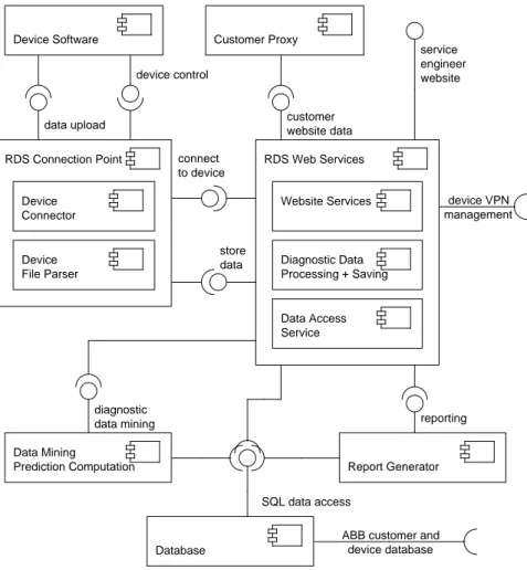
6 Architectures and Performance Models 48 6.1 RDS Architecture Overview . . . 48

6.2 Modeling Scope . . . 51

6.3 Baseline Model (Alternative 1) . . . 53

6.4 Initial Alternatives . . . 55

6.5 Second Iteration Alternatives . . . 60

6.6 Third Iteration Alternatives . . . 63

CONTENTS v 7 Predictions for an Architectural Roadmap 65 7.1 Simulator Configuration . . . 65 7.2 Model Simulation Results . . . 66 7.3 Architectural Roadmap . . . 67

8 Experiences with Palladio 69

8.1 Performance Modeling Using the PCM . . . 69 8.2 Using the Palladio-Bench Tool . . . 70

9 Future Work 72

10 Conclusions 73

Chapter 1

Introduction

In this thesis, we set out to create a performance model of a complex industrial system, which should help in selecting an architectural redesign that offers 10x more capacity. This Chapter first positions this thesis within the performance modeling research field in Section 1.1 and then explains ABB’s interest in this thesis in Section 1.2. Once this foundation is in place, we identify the goal of the work and formulate tasks to reach this goal in Section 1.3. The latter will also indicate the contributions and findings of this thesis. We close this introduction with an outline for the remainder of the thesis in Section 1.4.

1.1

Research Motivation

Traditionally, there exists a gap between performance modeling concepts and software modeling concepts, making it difficult for architects to use performance models without consulting an expert. This gap is now closing, making perfor-mance modeling more accessible. For example, UML annotations have been de-veloped to enable the transformation of UML software models to performance models, thereby removing the need for deep knowledge about performance mod-eling concepts such as queueing networks and Petri nets. In addition to these, strategies have been developed to deal with the state space explosion problem that limits the size of Markov chain based models. Finally, many techniques that underly software performance modeling are also used outside software en-gineering, where they are considered mature, and are frequently used. Yet, the industrial adaptation of software performance engineering seems to be low [SMF+_07].

Sankarasetty et al. suggest that a poor toolset is one of the factors that is holding back industry acceptance of software performance modeling. Indeed many tools offer either maturity or familiar modeling concepts (e.g., annotated UML), but fail to offer both. Furthermore, the number of case studies on real-istic, large industry software systems is limited. Industry might thus be right in its slow acceptance for it is not clear whether performance modeling can be easily integrated in existing software design and development.

CHAPTER 1. INTRODUCTION 2

1.2

Business Motivation

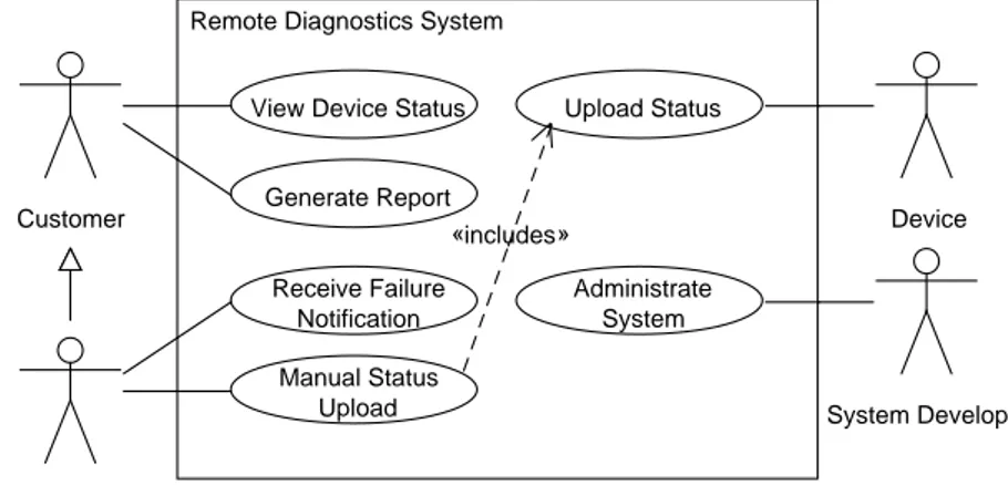
ABB’s Corporate Research Center (CRC) is engaged in a project to improve the performance of a remote diagnostic solution (RDS) by architectural redesign. The RDS under review is owned by one of ABB’s business units (RDSBU) and is used for service activities on deployed industrial equipment (devices). The RDS back-end is operating at its performance and scalability limits. Performance tuning or short term fixes (e.g., faster CPUs) will not sustainably solve the problems for several reasons. First, the architecture was conceived in a setting where time-to-market took priority over performance and scalability require-ments. Second, the number of devices connected to the back-end is expected to grow by an order of magnitude within the coming years. Finally, the amount of data received from the devices, which has to be processed, is also expected to increase by an order of magnitude in the same period. Both dimensions of growth will significantly increase the demands on computational power and storage capacity and justify architectural redesign.

The main goal of the architectural redesign is to improve performance and scalability of the existing system, while controlling cost. It is not feasible to identify the best design option by prototyping or measurements. Changes to the existing system would be required to take measurements, but the cost and effort required to alter the system solely for performance tests are too high because of its complexity. Further, it is difficult to tell whether a measured performance improvement is the effect of a parameter change or the effect of a random change in the environment [Jai91]. Therefore performance modeling is considered a key tool to ensure that the right architectural decisions are taken.

1.3

Goal and Contributions

Based on the problems outlined in the previous Sections we formulate the fol-lowing goals. Each goal is achieved by a set of tasks that is listed as a numbered list. Not all tasks fall within the scope of this thesis report. The thesis focusses on the actual performance model construction and validation. The other tasks have been carried out by the CRC project team or have been a joined effort between the author and the CRC project team. The goals and their tasks are listed below.

Goal 1. Identify the best architectural alternative to achieve a scalable speed-up of at least one order of magnitude to counter the experienced performance problems and to enable the predicted growth. The desired speed-up takes into consideration the performance improvements of hardware in the prediction pe-riod, so the speed-up has to be achieved purely in software.

Tasks towards Goal 1

1. Set performance and scalability requirements. (CRC project team) 2. Define architectural alternatives that improve performance and scalability.

(joined effort, Chapter 6)

4. Create a performance model of the current implementation of the RDS. (Chapter 6)

5. Obtain performance measurements of the current implementation to vali-date the created model. (CRC project team)

6. Validate the created model using measurements on the current implemen-tation obtained through experiments. (Chapter 6)

7. Predict the maximum capacity of the current system and alternative ar-chitectural designs. (Chapter 7)

8. Create an architectural roadmap. (joined effort, Section 7.3)

9. Prototype the critical parts of the envisioned architecture that could not be explored sufficiently with the performance model. (CRC project team) Goal 2. Evaluate the use of performance modeling for architectural redesign in industrial settings.

Tasks towards Goal 2

1. Survey the available performance modeling tools. (Chapter 4)

2. Maintain a list of lessons learned while applying the selected performance modeling technique and tool (Chapter 8)

This thesis reviews the literature for software performance modeling tools that are useful in an industrial setting in two steps. First, we identify the requirements for a tool to be used in an industrial setting. Then, we assess the tools for use in a multi-million dollar industrial architectural redesign project of an ASP.Net web service application. In the literature review we analyze the industrial applicability of more than 10 performance modeling tools and find that only some use formalisms close to software modeling and also offer the required functionality.

Next, we report on a realistic industrial performance modeling case study in which we use the Palladio-Bench performance modeling tool. We selected Palladio-Bench based on the aforementioned analysis. The case study shows how performance modeling can support decisions in the architectural redesign of a complex system that uses modern technologies. For in the case study, we have successfully built a performance model for a 300 KLOC system with a 15-20% prediction accuracy. Subsequently, we have used the model to analyze more than more than 10 alternative architectures. Thereby, we enabled ABB to take an informed decision on an architectural roadmap. Finally, the thesis reflects on the use of Palladio-Bench in an industrial setting.

1.4

Thesis Outline

The remainder of this thesis is structured as follows. In Chapter 2 we introduce the reader to scalability and performance modeling, and describe the state of the art. Related work is discussed in Chapter 3. Next, in Chapter 4 we select a performance modeling tool for use in our case study based on the requirements

CHAPTER 1. INTRODUCTION 4 that are identified in the same Chapter. Chapter 5 then describes the process we followed to create the performance model. The performance modeling and the studied architectural redesigns are the subject of Chapter 6. The results of evaluating the performance models and the selected architectural roadmap are both discussed in Chapter 7. We report on our experiences with performance modeling in industry using Palladio-Bench in Chapter 8. Finally, Chapter 9 out-lines plans and ideas for future work and we close the thesis with our conclusions in Chapter 10.

Chapter 2

Background & Foundations

In this Chapter we introduce the reader to the three dimensions of scalability in the AFK scale cube, which are used in the architectural alternatives of the case study. We also give an introduction to performance engineering and to software performance modeling. For the latter two subjects we discuss the most important techniques and give an overview of the state-of-the-art.

2.1

Scalability in Three Dimensions

The architectural alternatives considered in the case study in Chapter 6 are based on the theory of the AFK scale cube [AF09]. In this section, we give an overview of the principles of this scale cube, which was developed by Abbott and Fisher while working for AFK Partners.

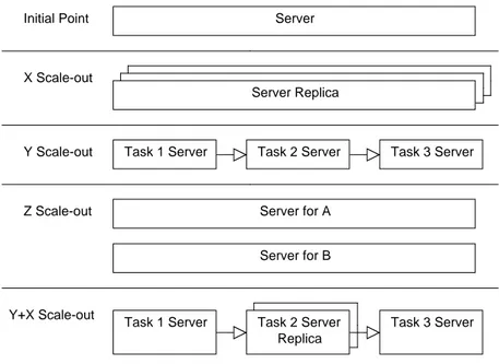
The AFK scale cube explains scalability as three fundamental dimensions, the axes of the cube. The initial point (0,0,0) where the axes intersect defines the point at which the system is least scalable. A system at this point is a monolithic application that cannot be scaled-out and which capacity can only be increased by increasing the capacity of the hardware. Moving the application away from the initial point along any of the axes increases the scalability, enabling the increase of capacity by spreading demand over multiple hardware resources. We will now discuss the principles for each axis. The axes are named X, Y, and Z, and are illustrated in Figure 2.1.

Moving along the X-axis (applying an X-split) can be done by cloning ser-vices and data. The cloning should be done in such a way that work can be distributed without any bias. For example, we may install a second server to publish an exact copy of our website.

Scaling in the Y-direction (applying a Y-split) we divide the work into tasks based on the type of data, the type of work performed for a transaction, or a combination of both. Y-splits are sometimes referred to as service or resource oriented splits. A Y-direction scale-out introduces specialization, i.e., instead of having one worker doing all the work, we have multiple workers all performing a task within the process. For example, splitting our website into application logic and a database will allow us to deploy these functions on two different machines.

When we scale along the Z-axis (apply a Z-split) we separate work based on

CHAPTER 2. BACKGROUND & FOUNDATIONS 6 Server Initial Point Z Scale-out X Scale-out Server Replica Server for A Server for B

Y Scale-out Task 1 Server Task 2 Server Task 3 Server

Y+X Scale-out

Task 1 Server Task 2 Server Replica

Task 3 Server

Figure 2.1: The three axes of the AFK scale cube

the requester (i.e., customer or client). This can be either by the data associated with a request, or the actions required by a request, or the person or system for which the request is being performed. For example, after replicating our server we may route customers from the US to a different server than customers from Europe, or clients who have account type A are served by a different server than clients who have account type B. When applying a Z-split we partition our data. That is, data is not mirrored between the replicas like when applying an X-split. It is also possible to move along several axes. For example, once the process is cut into tasks via Y-splits, replication via X-splits can be applied on individual tasks. This example is illustrated in Figure 2.1 where in the ‘Y+X Scale-out’ pane a replica has been added for task 2.

2.2

Performance Engineering

According to Woodside the approaches to performance engineering can be di-vided into two categories: measurement-based and model-based [WFP07]. The former is most common and uses testing, diagnosis and tuning once a running system exists that can be measured. It can thus only be used towards the end of the software development cycle. The model-based approach focusses on the earlier development stages instead and pioneered with the Software Performance Engineering (SPE1_{) approach by Smith (e.g., [WS98]). Like the name suggests,}

in this approach models are key to make quantitative predictions on how well an architecture may meet its performance requirements.

1_{In this thesis performance engineering should usually be read as the general field, if we} refer to the specific approach by Smith and Williams this will be pointed out or obvious from the context

Other taxonomies also exist, for example, Jain additionally considers simula-tion-based techniques as a separate category [Jai91]. On the other hand Kozi-olek dropped the distinction of categories entirely in the context of performance evaluation of component-based systems. He argues that most modeling ap-proaches take some measurement input and most measurement methods feature some model [Koz10]. This fading of the boundary between measurement-based and model-based techniques is illustrated by the work of Thakkar et al., who present a framework to support the automatic execution of the huge amount of performance tests needed to build a model from measurement data [THHF08]. Thakkar et al. also suggest that academia should invest in unifying and automat-ing the performance modelautomat-ing process usautomat-ing measurement-based techniques, as these are more widely accepted in the industry. To structure the discussions in this Chapter, we will use Woodside’s taxonomy of measurement-based versus model-based. In the following the measurement-based and model-based ap-proaches are introduced with their strengths and weaknesses. Section 2.3 will then dive deeper into performance modeling.

2.2.1

Measurement-based performance engineering

Measurement-based approaches prevail in industry [SMF+_{07] and are typically}

used for verification (i.e., does the system meet its performance specification?) or to locate and fix hot-spots (i.e., what are the worst performing parts of the system?). Performance measurement dates back to the beginning of the computing era, which means there is a complete range of tools available, such as load generators, to create artificial system workloads, and monitors to do the actual measuring. Examples of commercial tools are Mercury LoadRunner, Neotys Neoload, Segue SilkPerformer, and dynaTrace.

An example of a state-of-the-art measurement-based tool is JEETuningEx-pert, which automatically detects performance problems in Java Enterprise Edi-tion applicaEdi-tions [CZMC09]. After detecEdi-tion it proposes ways to remove the problems using rule-based knowledge of performance anti-patterns. JEETuning-Expert also helps us to understand why one would need a measurement-based system, for the JEE middleware behaviour is hard to predict and design time decisions might be changed during implementation. The JEE middleware hides the location of EJB components and takes care of much other non-functional behaviour. Unfortunately, JEETuningExpert knows only four anti-patterns at the moment, but recognizes these almost flawlessly.

Performance testing applies measurement-based techniques and is usually done only after functional and load testing. Load tests check the functioning of a system under heavy workload. Whereas performance tests are used to obtain quantitative figures on performance characteristics, like response time, throughput and hardware utilization, for a particular system configuration under a defined workload [THHF08].

We close our discussion of (pure) measurement-based techniques with two lists, enumerating the strengths, and the weaknesses of these approaches, respec-tively. Note that neither list is exhaustive, but together they enable making a trade-off with model-based approaches. Note that, in this thesis we aim to predict the performance of architectures that have not been implemented yet. Thus measurement techniques will only be instrumental in creating performance models and not used directly to find and ‘remove’ problems.

CHAPTER 2. BACKGROUND & FOUNDATIONS 8 Strengths

• Tool support; the maturity of the field comes with a lot of industry ready tooling,

• Acceptance of industry; in part due to the credibility of real measurements [THHF08, SMF+_07],

• Accuracy of results; observing the real system means that the problems and improvements measured are more accurate than those found in a model.

Weaknesses

• Not easily nor commonly applied in the early software development stages such as (architectural) design [WFP07],

• Performance improvement by code ‘tuning’ will likely compromise the orig-inal architecture [WS98],

• “Measurements lack standards; those that record the application and ex-ecution context (e.g. the class of user) require source-code access and in-strumentation and interfere with system operation.” [WFP07],

• Tools suffer from “a conflict between automation and adaptability in that systems which are highly automated but are difficult to change, and vice versa” [WFP07]. In the end, users have difficulty finding a tool that sat-isfies their needs and end-up inventing their own [WFP07],

• Every tool has its own output formats making interoperability a challenge [WFP07],

• It is difficult to correlate events in distributed systems. Determining causality within the distributed system is made even more difficult by the integration of sub-systems from various vendors, which is common practise [WFP07],

• Measurements are more sensitive to Murphy’s law than other approaches, making the amount of time required to do them less predictable. [Jai91, pg. 31],

• “The setting-up of the benchmarking environment as well as repeatedly executing test cases can run for an extended period of time, and consume a large amount of computing and human resources. This can be expensive and time-consuming.” [JTHL07],

• Test results obtained in a benchmarking environment may disagree with the performance of the production environment, because the former is often of a smaller scale than the latter. [JTHL07].

2.2.2

Performance engineering through modeling

The importance of performance modeling is motivated by the risk severe per-formance problems (e.g. [BDIS04]) and the increased complexity of modern systems, which makes it difficult to tackle performance problems at the code level. Considerable changes in design or even architecture may be required to mitigate performance problems. Therefore, the performance modeling research community tries to fight the ‘fix-it-later’ approach to performance in the de-velopment process. The popular application of software performance modeling is then to find performance issues in software design alternatives early in the development cycle, hence avoiding the cost and complexity of redesign or even requirement changes.

Performance modeling tools help to predict a system’s behaviour before it is built or to evaluate the result of a change before implementing it. Performance modeling may be used as an early warning tool throughout the development cycle with increasing accuracy and increasingly detailed models throughout the process. Early in development a model can obviously not be validated with the real system, then the model represents the designer’s uncertain knowledge. As a consequence the model makes assumptions that do not necessarily hold for the actual system, but which are useful for obtaining an abstraction of the system behaviour. In these phases validation is obtained by using of the model, and there is a risk of wrong conclusions because of the limited accuracy. Later the model can be validated against measurements on (parts of) the real system or prototypes and the accuracy of the model increases.

Jin et al. suggest that current methods have to overcome a number of challenges before they can be applied to existing systems that face architectural or requirement changes [JTHL07]. First, it must become clear how values for model parameters are to be obtained and how assumptions can be validated. Experience-based estimates for parameters are not sufficient and measurements on the existing system are required to make accurate predictions. Second, the characterization of system load in a production environment is troublesome due to resource-sharing (e.g., database sharing, shared hardware). Third, methods have to be developed to capture load dependent model parameters. For example, an increase in database size will likely increase the demands on the server CPU, memory, and disk.

Common modeling techniques include queueing networks, extensions to these such as layered queueing networks, and various types of Petri nets and stochas-tic process algebras [WFP07]. A recent and promising development is that of automatic performance model generation from annotated UML specifications; i.e., the architect or designer annotates his UML models and a performance model is automatically generated [WFP07]. We will discuss all of these in more detail in the next Section. We now close this Section with an overview of the strengths and weaknesses of performance modeling.

Strengths

• One can predict system performance properties before it is built [WFP07], • The effect of a change can be predicted before it is carried out [WFP07], • Automated model-building from specified scenarios with support of UML

CHAPTER 2. BACKGROUND & FOUNDATIONS 10 profiles early in the life cycle [WFP07].

Weaknesses

• “There is a semantic gap between performance concerns and functional concerns, which prevents many developers from addressing performance at all. For the same reason many developers do not trust or understand performance models, even if such models are available.” [WFP07], • Performance modeling often has high cost [WFP07],

• Models are only an approximation of the system and may omit details that are important [WFP07],

• It is difficult to validate models [WFP07],

• Models always depend on various assumptions. The validity of these is unknown in advance, nor is the sensitivity of the predictions to these assumptions known [WFP07].

• A good understanding of the system is required for performance model-ing, asking for the complete and accurate documentation of system behav-ior. But, in practise up-to-date and complete documentation rarely exists [THHF08].

2.3

Introduction to Performance Modeling

This Section introduces model-based performance engineering. We distinguish two categories of performance modeling approaches: analytical techniques and simulation techniques. Thakkar summarizes the difference between the two as: “Analytical techniques use theoretical models. Simulation techniques emulate the functionally of the application using a computer simulation whose perfor-mance can be probed” [THHF08]. However, no clear distinction can be made between simulation and analytics. Some constructed models may be evaluated both analytically and by using simulation.

Compared to simulation analytical techniques require more simplifications and assumptions, and this is especially true for models employing queues [Jai91, pg. 394]. Analysis techniques for performance models that are directly based on the states and transitions of a system generate a state space. Often these techniques cannot be used to model systems of realistic size due to the so-called state space explosion problem, in which the set of states to be analyzed grows exponentially with the size of the model [e.g., WFP07]. On the upside there are improvements to numerical solution methods for state spaces and the approximations they use [WFP07].

Simulation techniques allow for more detailed studies of systems than analyt-ical modeling [Jai91, pg. 394]. However, building a simulation model requires both strong software development skills and comprehensive statistical knowl-edge. Also, simulation models often require (much) more time to develop than analytical models. Jain reports that this (sometimes unanticipated) complexity causes simulation efforts to be cancelled prematurely more often than that they are completed [Jai91, pg. 393]. Over 15 years later Woodside still has a similar

opinion: “simulation model building is still expensive, sometimes comparable to system development, and detailed simulation models can take nearly as long to run as the system.” [WFP07].

Frank’s thesis tells us that simulations for layered queueing networks can take two orders of magnitude longer than analysis (i.e., hours vs. seconds) [Fra99, pp. 224–227]. Woodside notes however, that cheap, increasingly powerful com-puting makes simulation runtimes more agreeable. Yet, the complexity of sim-ulations remains high, which is illustrated by the fact that the runtimes listed in [MKK11] still are one to two orders of magnitude longer for simulations than for the layered queueing network analysis tool. Simulations take much longer due to the often substantial amount of runs that is required to gain statistical confidence in the results and the duration of model execution. Rolia et al. sug-gest therefore that an analytical model should always be preferred if it provides accurate predictions and does so consistently [RCK+_09].

2.3.1

Simulation versus process algebras

As an example of the trade-off between analytical and simulation techniques we report on the findings of Balsamo et al. [BMDI04]. They compare Æmilia, an analytical technique based on stochastic process algebras, and UML-Ψ (UML Performance SImulator), a simulation-based technique. Their work gives us insight in the strengths and weaknesses of the approaches when assessing per-formance on the architectural level.

Using the Æmilia architectural description language Balsamo et al. observed the aforementioned state space explosion problem for some of their scenarios. In these cases they experimented with UML-Ψ, which derives simulation models from annotated UML diagrams. This is one of the reasons that Balsamo et al. suggest that combining techniques can overcome limitations of single techniques and provide more useful results.

In UML-Ψ there exists a near one-to-one mapping from UML elements to simulation processes making it easy to construct the simulation-based perfor-mance model. The Æmilia model is also quite easily derived from the archi-tectural specification, but requires information on the internal behaviour of the components. In Æmilia it is also quite cumbersome to include fork/join systems, resource possession, and arbitrary scheduling policies. An advantage of UML-Ψ is then that it puts little constraints on the expressiveness of the software model. UML-Ψ allows to predict a wide range of different performance metrics. In Æmilia knowledge of the tool’s internal functioning is necessary to specify performance indices. Æmilia has the advantage however that it computes an exact numerical result whereas the simulation expresses results in confidence intervals and needs many samples (and potentially a lot of execution time) to compute means and remove bias.

Finally we should remember that at the moment the scalability of the Æmilia approach is limited due to the state space explosion problem. According to Balsamo et al. this problem limits the applicability of Æmilia in ‘real’ situa-tions. Solutions to the state space explosion problem require manual tuning of the generated models, which obviously requires skills and expertise. How-ever, the TwoTowers analytical tool associated with the Æmilia approach does have the added benefit that it can analyse system functionality in addition to non-functional aspects like performance.

CHAPTER 2. BACKGROUND & FOUNDATIONS 12

2.4

Performance Modeling Techniques

In the previous Sections we presented several performance engineering approaches and evaluated their strengths and weaknesses. This Section and Chapter 4 dis-cuss concrete techniques and tools. Here we will disdis-cuss popular techniques independent of their implementation and in Chapter 4 we compare several tools employing these and other techniques.

2.4.1

Queueing Network Models

Queueing Networks and Queueing Network Models (QNM) form a generic per-formance modeling technique that also has many applications outside software performance modeling and computer science. A thorough discussion of their application in computer science can be found in [LZGS84]. We based our short overview on that of Kounev et al. in [KB03]. First we define several parameters used in QNM:

interarrival time the time between the arrival of successive requests.

service time the amount of time the request spends at a server: the time it takes the server to handle the request.

queueing delay the time a request spends waiting for service in the queue. response time = queueingdelay + servicetime: the time a request spends

within the service station.

A queueing network is a collection of connected queues. Every queue is part of a service station and regulates the entry of requests or jobs into its service station. Requests are handled by the service station’s servers. Upon arrival at the station a request may be served directly if a server is available or if it causes a lower priority request to be preempted. Otherwise the request queues until a server frees up.

The queues might employ different strategies to decide which request is the next to receive service when a server becomes available; these strategies are called scheduling strategies. Typical strategies are first come first served, last come first served, processor sharing (processing power is equally divided among all requests and all requests are processed simultaneously), and infinite server (no queue ever forms, the server only introduces a processing delay). A service center with the infinite server scheduling strategy is also called a delay center.

A QNM is built by connecting queues. If from one point multiple routes may be followed, the likelihood of each route is specified with a probability. Requests may also return to a service station multiple times, in this case the service time is defined as the total amount of processing time required at the service station. Requests with similar service demands may be grouped in a class.

Measures typically derived from the evaluation of QNM are queue lengths, response time, throughput and utilization (of service stations). Several efficient methods exist to evaluate QNM, for example mean-value analysis. While QNM are very suitable for modeling hardware contention (e.g., contention for disk access), QNM are not very good at describing software contention. This limita-tion gave rise to the development of several extensions. In the next subseclimita-tion we describe one of the most popular extensions to queueing networks: layered queueing networks.

2.4.2

Layered Queueing Networks

A popular extension to Queueing Network Models (QNM) are Layered Queue-ing Networks (LQN). LQN for distributed systems are introduced in [FMN+_96].

LQN add support for (distributed) software servers, which are often ‘layered’: in distributed systems processes can act both as client and server to other pro-cesses. High-layer servers make use of services/functionality offered by servers at lower layers, and the delays at higher-layer servers depend on those at lower-layer servers.

Distributed systems may suffer from a bottleneck not caused by saturation of a hardware resource, but caused by a software server waiting for replies from lower level services: a software bottleneck. LQN can be used to find these problems by calculating service times of a process for its own execution, its requests to other servers and the queueing delays it experiences during those requests. Other performance issues that may be studied using LQN are the impact of different algorithms, load balancing, replication or threading, and an increase in the number of users. Replication and threading are techniques that may remove software bottlenecks. LQN can also be used for sensitivity analysis, for example, to determine the limit of multi-threading performance gains before the overhead (extra memory requirements for the heap, and execution stack) kicks in, or to measure the sensitivity to cache hit ratios [FMN+_96].

A LQN models a system as requests for service between actors or processes and the queueing of a messages at actors [WHSB01]. Actors are modeled as tasks and accept service request messages at an LQN entry. An LQN entry provides a description of a service provided by an actor, and models this service and its resource demands. Tasks can be compared to objects and entries to methods, this analogy makes LQN conceptually easier to understand for software developers than many other performance modeling techniques.

Each LQN entry may have its own resource demands or performance pa-rameters, for not all are expected to behave the same (e.g., a database read operation may be served more quickly than a write operation). Performance parameters also help deal with various types of distributions. The type of dis-tribution deeply affects delays, consider for instance disdis-tribution across nodes on a WAN versus distribution across several processors on a shared bus. Further, LQN models are able to represent software at various levels of detail. In its sim-plest form it can be an ordinary queueing model not showing any software detail, but LQN can also model every software module in the design, all interactions between modules, and the resource demands for each of these [WHSB01].

2.4.3

Queueing Petri Nets

An ordinary Petri Net is a bipartite directed graph consisting of places, shown as circles, and transitions, shown as bars. We give a formal definition from [KB03]:

Definition 1. An ordinary Petri Net (PN) is a 5-tuple P N = (P, T, I−, I+_{, M} 0),

where:

1. P is a finite and non-empty set of places, 2. T is a finite and non-empty set of transitions,

CHAPTER 2. BACKGROUND & FOUNDATIONS 14

Figure 2.2: An Ordinary Petri Net before and after firing transition t1 (taken

from [KB03]

3. P ∩ T = ∅,

4. I−, I+ _{: P × T → N}0 are called backward and forward incidence

func-tions, respectively,

5. M0: P → N0 is called initial marking.

I− _{and I}+_{, the incidence functions, specify the interconnection between}

places and transitions. Places may be input places or output places depending on whether there is an edge from the place to a transition (input place) or vice versa. Place p is an input place if I−(p, t) > 0 and an output place if I+_{(p, t) > 0.}

Each edge has a weight, which is assigned by the incidence functions. When a transition takes place it is said to fire. It then destroys N tokens from each of its input places, where N is equal to the weight of the edge between the input place and the transition. Transitions can only fire when all input places contain N tokens. Note that N is specific for each input place. Upon firing the transition creates tokens in output places, again the number of tokens created is dependent on the weight of the edge between the transition and the output place. An arrangement of tokens is called a marking and M0 gives the initial

arrangement of tokens in the Petri Net. An example of a simple Petri Net is shown in Figure 2.2. The example net has 4 places and 2 transitions, all edge weights are 1. The left of the figure shows the Petri Net before firing transition t1, the right half shows the situation after firing.

Petri nets have been extended on several occasions either to increase con-venience or expressiveness. A number of extension are combined in Colored, Generalized, Stochastic Petri Nets (CGSPNs), which add advanced timing con-trol and typing of messages. None of the extensions are suitable to represent scheduling strategies, the speciality of queueing networks. To overcome this Queueing Petri Nets (QPN) include some ideas from queueing networks [KB03]. In QPNs the places of CGSPNs are extended by adding a queueing place, which consists of a QNM service station and a depository for the storage of tokens (re-quests in queueing networks) that have been serviced. While the readability of the models is reduced by the QPN extension, it does increase the expressiveness of the models [TM06].

One way to model a software system in QPNs is described by Tiwari and Mynampati in [TM06]. They map software processes onto ordinary places. The

number of process tokens in these places represent the number of available pas-sive resource tokens (i.e., threads, connection pools, etc.). Transitions between places are defined so that they allow to a request token to move to the next queueing place when the right conditions are met.

Unfortunately, Petri nets are sensitive to the state space explosion problem inhibiting efficient analysis of large models. To alleviate this problem Falko Bause developed the HQPN (hierarchical QPN) formalism. In a HQPN model a queueing place might contain a whole QPN instead of a single queue. Queuing places are therefore known as subnet. This hierarchical nesting enables efficient numerical analysis and thereby alleviates the state space explosion problem [KB06]. However, when modeling systems of realistic size, the state space ex-plosion can still be problematic [TM06].

LQN vs. QPN

Tiwari and Mynampati report on their experience applying both LQN and QPN to a J2EE application in [TM06]. We report some of their findings to compare the relative merits of the techniques. They succeeded applying both techniques and both models gave similar performance results, but it is interesting that they observe LQN to be less accurate in modeling software contention of a system than QPN. The remaining trade-offs are as follows (all quoted from [TM06]):

• QPN can be used to analyze both functional and performance aspects of system. Whereas LQN gives only the performance measures of a system. • LQN can be analytically solved using the approximate MVA techniques with minimal resources; while QPN is analytically solved using Markov process thus requires resources that are exponential in the size of the model to produce exact results.

• LQN does not have any computational limitations, so can be modeled for any number of layers (tiers)/resources. Nevertheless the QPN computa-tion model becomes exponentially complex with addicomputa-tion of each ordinary place and queueing place.

• The LQN models can be used for modeling any number of concurrent user requests. However the QPN model cannot be used for large number of concurrent requests due to state space explosion problem.

• LQN supports both the open (geometric distribution) and closed requests. While the QPN is restricted only to modeling the closed requests. • LQN can be used to model synchronous, asynchronous and forward calls.

So messaging systems can also be modeled with LQN. QPN supports only synchronous calls.

• In QPN memory size constraints for performance can be modeled more accurately than in the LQN.

• LQN model consists of convenient primitives notations which makes LQN construction simple, convey more semantic information and guarantee that these models are well-formed (i.e. stable and deadlock free) [DONA1995 (citation theirs)]. On the other hand, the low level notations used in QPN give them added expressive power with some readability complexity.

CHAPTER 2. BACKGROUND & FOUNDATIONS 16

2.4.4

Palladio Component Model

The Palladio Component Model (PCM) is based on the roles and tasks within the component-based software engineering philosophy: component developer, architect, deployer, and domain expert. The component developer is responsible for developing software components. The architect combines these components to form a system, which is deployed by the deployer (i.e., system administrator and application manager). A domain expert specifies the usage of the system. We will now discuss the parts of the PCM in turn.

Component Repository

In the PCM, information about the available components and their interfaces is collected in the component repository. The component repository is cre-ated and maintained by the component developer(s). When a developer creates a component he should also specify its resource demands in a Service EFfect speciFication (SEFF). An important part of the SEFF is how the component uses its required interfaces. For example, a web page component SEFF may specify that the web page makes three calls to the database interface to read information. In addition, other resource requirements can be specified, for ex-ample, the amount of CPU cycles or time, or the number of threads required from a thread pool. Here a thread is an example of a software resource, which can be modeled in the PCM using passive resources (i.e., instead of processing resources such as a CPU).

System Model

Using the components from the component repository the architect can specify a system model. The architect selects the components he wishes to use and connects required interfaces to matching provided interfaces. Systems generally include at least one provided system interface to make its services available. Likewise systems may of course have required system interfaces to connect to other systems.

Allocation Model

The deployer of the system creates the allocation and resource environment diagrams. The resource environment diagram specifies the available hardware resources such as servers and their CPUs and memory. The allocation diagram then maps the system components to containers in the resource environment (i.e., typically servers).

Usage Model

Finally, the typical use of the system is specified by the domain expert in the usage model. The domain expert specifies usage scenarios and the amount of users or processing requests (in the case of batch jobs). The usage model may be modified to test system behaviour under various loads.

2.5

State-of-the-Art

In order to present a comprehensive state-of-the-art of software performance evaluation, that is, briefing the reader on techniques and tools beyond those used in this report, we first discuss a number of surveys, which can also be used as guide for further reading. After these, we discuss automated performance modeling, one of the field’s frontiers. The contents of this Section should help the reader to judge the research field in which the thesis work was carried out. In his survey of the state of the art and the future of software performance engineering, Woodside calls the state ‘not very satisfactory’ [WFP07]. Often heavy effort is required to carry out the performance engineering processes; there is a semantic gap between functional and performance concerns; and developers find it difficult to trust models: these are just three of the issues he identifies [WFP07]. He suggests that measurement and modeling based approaches have to be combined to ensure further progress.

Becker et al. and Koziolek surveyed performance evaluation for component-based systems in [BGMO06] and [Koz10]. They analyze the strengths and weak-nesses of component-based software performance modeling tools and provide recommendations for future research. Koziolek blames immature component-based performance models, limited tool support for these and the absence of large-scale industrial case studies on component-based systems for the sparse industrial use of performance modeling for component-based systems [Koz10]. Out of the 13 tools he surveyed only four are rated to have the maturity required for industrial application, but the conclusion does note a significant advance in maturity over the last ten years of performance evaluation for component-based systems [Koz10].

The earlier findings of Balsamo et al. are similar. They note that despite of newly proposed approaches for early software performance analysis and some successful applications of these, performance analysis is still a long way from being integrated into ordinary software development [BDIS04]. And while no comprehensive methodology is available yet, they suggest that the field of model-based software performance prediction is sufficiently mature for approaches to be put into practice profitably.

2.5.1

Automatic Performance Modeling

Various approaches that automate (part of) the performance modeling process have been proposed over the years. Automation should make performance mod-eling faster and more accessible to software designers [WHSB01].

Model extraction from traces

A first category of approaches contains methods to extract performance models from execution traces. The work by Litoiu et al. describes one of the first trace-based model creation tools for ‘modern’ applications [LKQ+_{97]. They}

create layered queueing network (LQN) models using traces from EXTRA (a commercial tool then part of IBM’s Visual Age suite). The EXTRA trace files may be imported into another IBM tool called DADT (Distributed Application Development Toolkit) to explore the impact of design and configuration changes on application performance.

CHAPTER 2. BACKGROUND & FOUNDATIONS 18 In 2001 Woodside et al. presented a prototype tool to automatically con-struct layered queueing network models of real-time interactive software using execution traces of performance critical scenarios [WHSB01]. The extracted models may be maintained throughout the development cycle taking new traces gathered from the evolving system implementation. A limitation is that the traces have to be provided as angio-traces, a specific trace format.

Israr et al. propose the System Architecture and Model Extraction Technique (SAMEtech), which can use traces in standard formats to derive LQN models [IWF07]. SAMEtech can also combine information from multiple traces into one model and features a linearly scaling algorithm for large traces. Limitations include the inability to detect the joining of flows and synchronization delays associated with forking and asynchronous messages. Also workload parameters for the models are not automatically extracted.

Software design model transformation

In the second category we find several approaches that provide automatic trans-formation of software design models (e.g., UML models) to performance models, but to our knowledge, no robust, industry-ready tools are available yet. One of the problems is that it is difficult to translate incomplete or inconsistent design models into useful performance models.

Balsamo et al. transform UML use case, activity and deployment diagrams to multi-chain and multi-class queueing networks [BM05]. The UML diagrams have to be annotated with the UML profile for Schedulability, Performance and Time specification (SPT profile) to include the additional information required to specify a performance model. Unfortunately, the UML software model must be constrained to avoid the need for use of simulation or approximate numer-ical techniques. Petriu presents a similar automatic transformation of a UML specification into a layered queueing network [Pet05].

The work by Woodside et al. uses a common intermediate format, the Core Scenario Model (CSM), towards a framework for the translation of software de-sign models to performance models, both in various notations [WPP+_{05]. The}

PUMA framework is more flexible than other model transformations: one can plug software design tools into the framework as sources and feed output to dif-ferent performance modeling tools. In [WPP+_{05] input from UML 1.4 is used to}

create the CSM from which LQN, Petri Nets and QNM are built. The authors argue that a framework such as PUMA is a requirement for the practical adop-tion of performance evaluaadop-tion techniques, as it does not tie a developer to “a performance model whose limitations he or she does not understand”. However, PUMA is limited by the diversity of proprietary features vendors include in the XMI standard used to serialize UML software design models [WPP+_05].

Zhu et al. present a model-driven capacity planning tool suite called Revel8or to ease cross platform capacity planning for component-based applications in [ZLBG07]. The Revel8or suite consists of three tools: MDAPref, which derives QNM from annotated UML diagrams; MDABench, which can generate custom benchmark suites from UML software architecture descriptions (also discussed in [ZBLG07]); and DSLBench, a tool similar to MDABench targeted to the Mi-crosoft Visual Studio platform. The results of the benchmarks may be used as parameter values in performance models, therefore it is of great value having a benchmark that is representative of the application under development.

Un-fortunately, neither [ZBLG07] nor [ZLBG07] includes empirical data supporting the claimed productivity gains, nor are the tools publicly available.

Feedback into software design

The third and final category of automation approaches automatically ‘solves’ performance problems. For example, utilizing the automatic recognition of per-formance anti-patterns in software architectures, Cortellessa et al. introduce a framework to automatically propose architectural alternatives [CF07]. The framework employs LQN models to generated the architectural alternatives. The goal of the automation is to relief architects of interpreting the results of performance analysis and the selection of the right architectural alternative based on this analysis. The prototype tool used in [CF07], however, still requires human experience and manual intervention in some steps.

The work by Xu automates the entire performance diagnosis and improve-ment process with a rule-based system that generates improved models [Xu10]. Using the approach a large number of different design alternatives can be ex-plored quickly. Through the PUMA approach described earlier in [WPP+_{05] a}

LQN model is obtained. The models are evaluated with the LQNS tool and rules then generate improved performance models, which can in turn be (manually) translated back to improved software design models. A prototype tool called Performance Booster is evaluated on multiple small (of which one industrial) case studies. Eventually Performance Booster is aimed to be integrated in the PUMA toolset. Current limitations include the disregard of memory size effects, overhead costs of multi-threading, multiple classes of users, and the inability to suggest introduction of parallelism.

Chapter 3

Related work

In this Chapter, we describe the relevant work that has been done by fellow researchers and is related to the topic of this thesis. The discussion consists of three parts. First, we focus on publications that are related to our survey of tools and techniques and our tool selection. Second, we treat studies that discuss systems with architectures that are in some way similar to the RDS. Finally, we discuss case studies that are related for other reasons.

3.1

Survey and Tool Selection

Several recent surveys review performance modeling tools, with a focus on model-based prediction [BDIS04], evaluation of component-based systems [BGMO06, Koz10], and analysing software architectures [Koz04]. An outlook into the fu-ture of, and directions for fufu-ture research in software performance engineering are given in [WFP07]. These surveys differ from this thesis by not studying the applicability of the tools to industrial systems. Jain’s 1991 landmark book still provides relevant guidance for selecting and applying performance modeling techniques [Jai91]. The book, however, does not include recent tooling.

Other work evaluates a limited number of tools and mainly focusses on ac-curacy and speed of these. Balsamo et al. study the benefits of integrating two techniques based on stochastic process algebras and simulation towards perfor-mance analysis of software architectures and also discuss the relative merits of both approaches in their own right [BMDI04]. Similarly, Tiwari and Myanam-pati compare LQN and QPN using the LQNS and HiQPN tools to model the SPECjAppServer2001 benchmark application [TM06]. Meier’s thesis compares the Palladio and QPN model solvers after presenting a translation from PCM to QPN. The evaluation is done in several (realistic) case studies and finds that the QPN solver is up to 20 times more efficient [Mei10] [subsequent publication in MKK11].

In an empirical study the effort and industrial applicability of the SPE-ED and Palladio modeling tools is investigated using student participants. The first report on this study finds that creating reusable Palladio models requires more effort, but is already justified if the models are reused just once [MBKR08b]. During later analysis of the empirical data the authors find that the quality of the created models is good and the usability of the tools by non-experts is

promising [MBKR08a]. The thesis of Koziolek includes a study that is similar to that of Martens et al., but is practically superseded by the latter [Koz04].

All above works show trade-off analysis similar to ours, but are often solely of academic nature. In this thesis, we additionally have industrial requirements for selection, e.g., tool stability, user-friendliness, and licensing.

3.2

Web Service Architecture Modeling Studies

A performance modeling tool intended for use early in the development cycle of SOAs is presented in [BOG08]. Among the suggested applications are evaluation of architectural alternatives and capacity planning. The tool produces SOA performance models from existing architectural artifacts (e.g. UML sequence and deployment diagrams), which may significantly reduce the cost of model creation. Brebner et al. later (presumably) extend the same tool and provide examples of the application of the approach [BOG09]. Unfortunately, little details are provided on the tool’s capabilities, and to our knowledge the tool is not publicly available. Recently, the authors presented a case study modelling the upgrade of an enterprise service bus (ESB) in a large-scale production SOA [Bre11]. Based on this experience they found that: models do not have to be complex to be a powerful tool in real projects; models can be developed incrementally, adding detail as required; a lack of information on the system can be overcome by building multiple alternative models and selecting the best fitting model; and if not enough information exists to build a comprehensive model covering the entire system, multiple specific models may be build to explore different parts of the system.

Bogardi et al. published a series of papers on performance modeling of the ASP.NET thread pool [BMLC07, BMLCH07, BMLS09, BMLC09] cumulating to [BML11]. In this final publication they present an enhanced version of the mean-value analysis evaluation (MVA) algorithm for queueing networks, which models the ASP.NET thread pool more accurately than the original MVA al-gorithm. The current practical implications of the work remain unclear. In part, because the modeling of the global and application queue size limits has not been completed yet, while these limits are identified as performance factors [BMLC07].

A model to assess the scalability of a secure file-upload web service is has been constructed in the PEPA process algebra by Gilmore and Tribastone. They can predict the scalability easily for large population sizes without having to construct the state space and thus avoid the state space explosion problem [GT06].

Urgaonkar et al. present a QNM that predicts the performance of multi-tier internet services for various configurations and workloads. The average predicted response times are within the 95% confidence interval of the measured average response times. They also find that their model generalizes to any number of heterogeneous tiers; is designed for session-based workloads; and includes application properties like caching effects, multiple session classes and concurrency limits [UPS+_05].

A case study on the SPECjAppServer2001 by Kounev and Buchmann demon-strates that QPN models are well suited for the performance analysis of e-business systems. One of the advantages they note is that QPNs integrate the

CHAPTER 3. RELATED WORK 22 modeling of hardware and software aspects [KB03]. Later the study is repeated on the new version of the benchmark application, SPECjAppServer2004, us-ing improved analysis techniques. Then the system is modeled entirely and in more detail, improving the accuracy and representativeness of the results [Kou06b, Kou06a].

Smith and Williams demonstrate their SPE approach and the associated SPE-ED tool in several case studies in their book [SW02], which also provides general practical guidance for the performance engineering process. One of the case studies investigates the performance impact of new functionality on an (imaginary) airline website [SW02, Chapter 13].

3.3

General Performance Modeling Studies

While many case studies in papers presenting tools and approaches are limited to ‘toy’ problems [e.g., SBC09], some are interesting and close to our work. For ex-ample, a three-tier web store modeled in Palladio and then implemented in .Net shows that the Palladio approach might be appropriate for our system [BKR07]. Gambi et al. also model a three-tier web architecture, but do so in LQNs while presenting a model-driven approach to performance modeling [GTC10]. Liu et al. present an approach to model the architecture of component-based sys-tems in QNM and validate their work on an EJB application. They find that performance predictions were often within 10 percent of measurements on im-plementations (for example systems). What makes their work relevant is that its authors believe the approach is general and could extend to the .Net component technology [LGF05]. Unfortunately, to the best of our knowledge, the work is not supported by tools or extended in later work. Next, Xu et al. developed a template-driven approach for the LQN modeling of EJBs, which they use to correctly predict saturation of CPU and thread-pool resources [XOWM06]. It is suggested that an approach similar to theirs could be applied to .Net, but we have not found any work in this direction. The work by Koziolek et al. shows that model-driven performance evaluation also works for large and complex in-dustrial process control systems [KSB+_{11]. The thesis of Ufimtsev proposes}

a framework to model the performance of middleware-based systems, such as J2EE and Com+/.Net, and includes a case study applying this technique to an industry-benchmark J2EE application, ECPerf [Ufi06]. The approach in Ufimt-sev’s thesis is interesting because it specifically addresses the fact that in web systems as little as 3% of execution time may be spend in ‘user’ code, while the rest of the time is spend in the application framework’s code.

However, all these works have in common that they are limited in detail and chiefly used to demonstrate or showcase a technique. Whereas this thesis investigates how the techniques may be used in an industrial setting.

Other case studies model industrial systems, which differ significantly from ours: Gaonkar et al. create a simplified model of a Lustre-like file system in M¨obius [GKL+_{09]. Huber’s thesis models a storage virtualization system for}

the IBM System/z experimenting with Palladio outside the targeted modeling domain of business information systems [Hub09] [published in HBR+_{10]. Rolia}

et al. show that LQM are more suitable for modeling complex systems than QNM by means of an elaborate industrial case study of the SAP ERP system [RCK+_{09]. Franks et al. find that analytical results of a LQN evaluation are}

within a few percent of simulations in a case study of an air traffic control system of realistic complexity and size [FAOW+09]. Jin et al. also use LQN and predict the scalability of a legacy information system, while presenting their BMM approach to performance prediction for legacy systems that need to adapt to new performance requirements [JTHL07].

Finally, [SMF+07], and [Mon10] provide experience reports based on long term experience [SMF+_{07], and introduce performance modeling [Mon10].}

Un-like this thesis these reports do not show the case studies that led to this expe-rience.

Chapter 4

Performance Modeling

Tools

One of the tasks that we have identified in the introduction is to survey the available performance modeling tools. This Chapter reports on the results of this survey, and then discusses our selection of a performance modeling tool to model the RDS. To carry out these tasks we have tried to answer the following questions.

1. What are the common performance engineering tools and their pros and cons?

2. What performance modeling tools exist that are applicable to web service systems?

Various tools to construct performance models exist. During our survey we looked for tools based on several criteria. First, the tool should show appli-cability to performance modeling of software architectures, this excludes some of the more mature low-level tools. Second, it must be released and available, this excludes many academic tools described in published research. Finally, it should be mature and somewhat stable, again a requirement often not met by tools presented in research publications. We will now briefly motivate why we excluded some of the well known performance modeling tools to illustrate our selection process.

GreatSPN1_{and ORIS}2_{are low-level Petri Net modeling tools and do not offer}

the expressive power of QPNs like QPME. Further, while state space reduction mechanisms are in place, the tools are still sensitive to state space explosion.

ArgoSPE3can generate Stochastic Petri Nets in GreatSPN format, but aims to ease the modeling of software systems by offering a UML ‘interface’. Unfor-tunately, it is based on an obsolete version of ArgoUML. Furthermore, the ad-vantage of the use of UML is limited by the sparse support for UML constructs. For example, there is no support for component diagrams. Finally, judging by the project home page, the tool doesn’t seem to be actively maintained.

1_{GreatSPN: http://www.di.unito.it/∼greatspn/index.html} 2_{ORIS: http://www.stlab.dsi.unifi.it/oris/}

3_{ArgoSPE: http://argospe.tigris.org/}

TwoTowers4 _{isn’t actively updated either. The last new version dates five}

years back. The specification of models is cumbersome because of the textual notation used. Finally, the approach suffers from the state space explosion problem, limiting model scalability [BMDI04].

Hyperformix5promises to be an all-round scalability solution including load testing, instrumentation, measurement, and model tooling. However, the tool is very expensive and the exact features and supported use cases are not clear. Furthermore, specific tooling for load testing, and instrumentation and mea-surement was already acquired by ABB when the thesis work commenced.

PEPA tools6_{offers a powerful process algebra. Comprehensibility of process}

algebras and mapping to software architecture concepts is, however, problem-atic. In addition PEPA tools uses a textual notation and a solver that is less efficient than LQNS, which also has a textual notation but offers more natural mapping of concepts.

SHARPE7 _{has not been updated in 10 years. And does not provide}

archi-tectural support, but only low-level modeling.

Finally, PRISM8only has support for Markov chains, which makes it difficult to model queueing effects.

In the end we selected six tools that seemed mature enough and promised to fit our architectural modeling problem. These tools will be described in more detail. The discussion in this Section will be rather neutral, but it forms the foundation for our tool selection in Section 4.7. For information on other tools, recall from Section 2.5 that surveys of the state of the art may be found in [BDIS04, BGMO06, Koz10] and [Koz04, Appendix A].

A quick overview of the considered tools is included in Table 4.1 on page 26. Each tool is discussed in more detail in the following sections. The discussions start with a short introduction and then contain the following parts:

1. Advantages – positive reasons for selecting this tool.

2. Inputs – specific input requirements for the model and modeling process. Of course, all tools will require an architecture to model, performance goals, and performance measurements to instantiate model parameters on top of these.

3. Time required – qualitative assessment of the required effort for modeling. 4. Accuracy – qualitative assessment of the quality of the predictions made

by the tool.

5. Assumptions – important assumptions made by the tool, e.g., limiting its applicability.

6. Limitations – reasons for not selecting this tool; besides timeliness we also wish to model memory and storage requirements of the system, support for this is also indicated here if present.

4_{TwoTowers: http://www.sti.uniurb.it/bernardo/twotowers/} 5_{Hyperformix: http://www.hyperformix.com/}

6_{PEPA tools: http://www.dcs.ed.ac.uk/pepa/tools/}

7_{SHARPE: http://people.ee.duke.edu/∼kst/software packages.html} 8_{PRISM: http://www.prismmodelchecker.org/}

CHAPTER 4. PERFORMANCE MODELING TOOLS 26 Name Li ce ns e S of tw are M o de l P er for man ce M o de l An aly sis / S im ul at ion S tud ies Case St u di es S tat u s J a v a M o de li n g T o ol s G NU GP L -Q NM b ot h [B C09, SB C09, CS M 11] [SB C09, R CK +09] (Q NM re lat ed: [UPS +05] st ab le La y er ed Q ue ue ing Net w or k S olv er E v al u at ion on ly (t ex t) LQ N b ot h [W o o02, F M N + 96] [TM 06, J THL07, G TC10] (r el at ed : [Xu10] ) st ab le P all ad io-Be nc h F re e do wn -load P all ad io Comp o-n en t M o de l (PC M) P CM or LQ N b ot h [BK R07, M BK R08a, M BK R08b , BK R09, BK K 09] [Hub 09, HBR +10, K SB +11] st ab le / mat u re M ¨ob iu s Comm er ci al for non -acad em ic u se S AN, Bu ck -et s & Bal ls, P EP A-n et s st o chas tic ex ten sion s to P et ri Ne ts , M ark o v ch ai ns (+ ex ten si on s) , an d st o chas -ti c pr o cess al geb ras si m u lat ion, an aly sis for som e [CG M + 07, CG K + 09, San 10, G K L +09] ??? mat u re S PE -E D Comm er ci al M S C, E x-ec ut ion gr aph s Q NM b ot h [S mi 86, W S98, S W 02, M BK R08b , M BK R08a] [W S98, S W02] st abl e / mat u re Q PM E O p en sour ce -Q PN si m ul at ion [K S M10, K D B06, K B06] [K B06, K ou06a, K ou06b , K B03] acad em ic / st ab le (?) T ab le 4. 1: Ov erv iew of cons id er ed to ol s.