www.transportekonomi.org
When should infrastructure assets be renewed?
The economic impact of cumulative tonnes on railway
infrastructure
Jan-Eric Nilsson, VTI, Stockholm, Sverige
Kristofer Odolinski, VTI, Stockholm, Sverige
Working Papers in Transport Economics 2020:4
Abstract
This paper provides empirical evidence on the optimal timing of rail infrastructure renewal. Using an econometric approach on data from the Swedish railway network, we establish a relationship between cumulative tonnes and maintenance costs, as well as between
cumulative tonnes and infrastructure failures that cause train delays. Together with average values on delay hours per failure and assumptions on passengers per train, we perform example calculations on the optimal timing for a track renewal. This timing will depend on the case considered, such as whether traffic intensity is high or low. Empirical evidence on the relationship between line capacity utilisation and delay time can provide more robust estimates for the different cases considered by an infrastructure manager. Still, the results in this paper is a significant step towards a usable cost-benefit analysis model for the timing of rail infrastructure renewals.
Keywords
Railway; Infrastructure; Optimization; Renewal; Maintenance; Train Delays
JEL Codes H54; L92; R49
1
1. Introduction
Construction of new railway infrastructure requires significant amounts of resources. Moreover, wear and tear make it necessary to carry out maintenance and eventually to renew the assets over their life cycle, which over time also add up to large costs. The Swedish Transport Administration (Trafikverket), also referred to as the Infrastructure Manager (IM), has spent between SEK 7 and 10 billion each year on rail infrastructure maintenance and renewals since 2010. In addition, malfunctioning infrastructure caused between 12 000 and 21 000 train delay hours per year during the 2013-2018 period on Sweden’s railway network (Gummesson, 2019).1
To economise on resources, the infrastructure manager (IM) must implement maintenance activities at the right time. A cost minimizing plan must balance the costs for undertaking a costly renewal against the costs for day-to-day maintenance and the railway traffic disturbances emanating from poorly functioning infrastructure. Since both day-to-day maintenance and the number of infrastructure failures that cause train delays increase over time it will eventually be better to allocate resources for a costly renewal.
Cost-Benefit Analysis (CBA) models for rail infrastructure investment appraisal are today available in many countries; see for example guidelines for Britain (DfT, 2018), Sweden (Trafikverket, 2018) as well as a review of Sweden’s guidelines by Andersson et al. (2018). the corresponding decision support for maintenance and renewal is much less developed. The incomplete understanding of how costs increase with an ageing infrastructure is one of the main challenges for developing a well-designed approach for maintenance appraisal. In view of the large resources spent on infrastructure maintenance and renewal, and the amount of train delays caused by infrastructure failures, this is a major shortcoming.
The purpose of this paper is to provide empirical evidence on the optimal timing of rail infrastructure renewal. To do this, we estimate how both track maintenance costs and the risk for infrastructure failures that cause train delays increase over time. This is based on information about costs, traffic and infrastructure characteristics between 1999 and 2016, and information on the number of failures from 2003 to 2016. With this information at hand, the most important variables for building a usable CBA model for the timing of renewals will be available.
Traffic accumulates on each track section over time but once the tracks are replaced, accumulated traffic goes back to nought on that part of the infrastructure. While comprehensive information about the timing of track renewal is available, the timing of renewals for other technical systems, such as signals, and electrical installations is not. This means that the information about accumulated use of these subsystems is incomplete. It is, however, reasonable to expect a degree of
2 correlation in the age of different types of plant. One reason is that there may be scope economies in replacing all or at least several asset classes at the same time. Another reason is that the annual number of costly quality (safety) inspections increase with asset age. Even if electricity, signalling, telecommunications and other installations are not replaced at the same time as tracks, their rate of replacement may still be a function of quality and (ultimately) time.
An extensive literature is concerned with establishing an appropriate timing of renewals and maintenance activities. Gaudry et al. (2016) proposes a framework for optimizing maintenance and renewals of rail infrastructure. Andrade and Teixeira (2011) consider activities with respect to track geometry while Sousa et al. (2018) apply multi-objective optimization for a case study in Portugal (minimizing total cost being one of the objectives). Moreover, Caetano and Teixeira (2014) use a life-cycle cost approach to find the optimal renewal timing for ballast, rail and sleepers. Yoo and Garcia-Diaz (2008), Sathaye and Madanat (2011), de la Garza et al. (2011), Gu et al. (2012), analyse the optimization of maintenance and resurfacing activities of road infrastructure, not to mention the seminal work by Small et al. (1989), who presents an equilibrium pricing and road infrastructure investment model.
Most of these models are based on mechanistic (bottom-up) approaches. This is often also the case for the literature on the prediction of railway failures. Examples are Hokstad et al. (2005), and Podofillini et al. (2006). However, there are also examples of econometric (top-down) approaches, including Schafer and Barkan (2008), and Parra et al. (2012). Yet, studies on railway infrastructure failures often consider one type of failure at a time, such as deviations in track geometry (Zarembski et al. (2016)), broken rails (Hokstad et al. (2005), Schafer and Barkan (2008)), weld failures (Zhao et al. (2006)). The prediction of failures is then typically used to calculate an optimal interval for inspections and/or maintenance activities. In general, these mechanistic (bottom-up) approaches are based on assumptions and cost relationships – for example, the actions needed to remedy the damage and unit costs of these actions – which may not be applicable to other railways and traffic situations.
This paper applies an econometric top-down approach for establishing the relationship between cumulative traffic and maintenance costs as well as infrastructure failures for the different types of infrastructure assets that are necessary for operating railway traffic. The strength of this approach is not only that it is solidly based on a panel of comprehensive data but also that it makes it possible to put few restrictions on the elasticities of production, such as accounting for any potential scale economies in maintenance activities. To the authors’ knowledge, a top-down econometric model estimation on actual data that captures costs for both delays and maintenance, as well as costs for renewals, has not been done before.
3 After having presented the method in section 2 and data in section 3, the results from model estimations are summarised in section 4. These results are used for making example calculations on the optimal renewal time in section 5 while section 6 concludes.
2. Methodology
As time pass, traffic using a track section adds up to accumulated traffic, which makes the asset come closer to the end of its life cycle, despite reoccurring maintenance activities such as rail grinding and minor replacements. Since two lines may be built to the same standard but not used by the same number of trains, or used by trains of differing weight, it is necessary to account for this distinction. This paper therefore uses a cumulative traffic measure in the empirical estimations, which is also used in both Odolinski (2019) and Gaudry et al. (2016) as an indicator for the overall condition of railway infrastructure. In general, cumulative traffic is a useful measure for an IM deciding whether to renew or keep maintaining the rail infrastructure asset.
Railway infrastructure comprises four asset types, subsequently indexed by 𝑔; track super- and substructure, power supply, signalling and a telecommunication system. In the subsequent analysis, focus is on the first category, but with access to lucid data we will also consider the aggregate of the other three, meaning that 𝑔 = 1, 2.
Quality may deteriorate in different ways for the two categories. It is not obvious why for instance the cost for power supply maintenance would be related to the weight of trains. As noted previously, there may still exist a degree of correlation since it may be beneficial to replace other assets when tracks are renewed. But even if the assets are not replaced at the same time, the frequency of inspections increase with the age of the overhead lines and pylons. In the same way, the number of failures of these systems may increase over time. This means that it is reasonable to expect a link between time and quality deterioration also for assets other than tracks and structures. It is still not obvious that clock-time is the best way to measure age. The reason is that traffic accumulates at different rates on different parts of the railway network and are renewed after different number of years. For this reason, cumulative tonnage (𝑄) is used for registering how maintenance and delay costs change over time.
Section 2.1 sets out an analytical model for establishing principles for infrastructure renewal while sections 2.2 and 2.3 formulates the empirical models for estimating the rate of increase of maintenance costs and delay costs, respectively.
4
2.1 Analytical model
Over time, railway infrastructure deteriorates in quality. Each year 𝑡, maintenance activities are carried out to keep the line in shape and to reduce the risk for train services being affected by deteriorating quality. Even though the extent of preventive maintenance increases over time, the infrastructure will occasionally and increasingly malfunction and disturb trains, generating delay cost 𝐷𝑡. This triggers corrective as well as preventive maintenance which costs 𝑀𝑡. In general, both these costs increase with accumulative use, i.e. 𝜕𝑀𝑡
𝜕𝑄
⁄ ≥ 0 and 𝜕𝐷𝑡 𝜕𝑄
⁄ ≥ 0. Maintenance will, in other words, prolong the lifetime of the asset, but it is still coming closer to the end of its life cycle as time goes by. It is eventually beneficial to renew at time 𝑡 = 𝑇 at cost 𝑅.
Disregarding possible budget constraints etc., the IM’s objective is to minimize life cycle costs (𝑉) by establishing the optimal 𝑇 using eq. (1), where 𝐴(𝑇) = 𝑀(𝑇) + 𝐷(𝑇) is maintenance and delay costs over the asset’s life cycle, 𝑟 is the discount rate, and the denominator is used to express the present value cost at 𝑇 for all future renewal cycles.
min 𝑇 𝑉 =
𝐴(𝑇)+𝑅𝑇
(1−𝑒−𝑟𝑇̅) (1)
Taking the derivative of (1) with respect to 𝑇 and setting to zero, results in eq. (2):
𝜕( 𝐴(𝑇) (1−𝑒−𝑟𝑇̅)) 𝜕𝑇 = − 𝜕( 𝑅𝑇 (1−𝑒−𝑟𝑇̅)) 𝜕𝑇 (2)
Eq. (2) can be evaluated to give
(𝜕𝐴(𝑇) 𝜕𝑇 )(1−𝑒 −𝑟𝑇̅ )−𝐴(𝑇)𝑟𝑒−𝑟𝑇̅ (1−𝑒−𝑟𝑇̅)2 = 𝑅𝑇𝑟𝑒−𝑟𝑇̅ (1−𝑒−𝑟𝑇̅)2 (3)
Let 𝑎 = 𝑟𝑒−𝑟𝑇̅ be the factor representing how costs change from one year to another and 𝑏 =1−𝑒1−𝑟𝑇̅ be the discount factor for the infinite cycle of future renewal intervals 𝑇̅ (see for example Andersson et al., 2016). Eq. (3) can then be expressed in the following way:
𝜕𝐴(𝑇)
𝜕𝑇 − 𝐴(𝑇)𝑎𝑏 = 𝑅𝑇𝑎𝑏 (4)
Eq. (4) establishes that it is optimal to renew when the increase in the discounted maintenance and delay costs is equal to the gradual reduction in discounted renewal costs over time. This demonstrates
5 the necessity to establish how maintenance and delay costs increase over time and as traffic accumulates.
2.2 Empirical model: Traffic and costs
Maintenance costs on asset 𝑔 and track section 𝑖 in year 𝑡 are considered to be a function of cumulative tonnes (𝑄𝑖𝑡) and a set of infrastructure characteristics (∑𝐿𝑙=1𝑋𝑙𝑖𝑡) such as track length, rail weight, quality classification and average number of tracks. Specifically, the platform for the empirical analysis on maintenance costs is
𝑀
𝑔𝑖𝑡= 𝑓(𝑄
𝑖𝑡, ∑
𝐿𝑙=1𝑋
𝑙𝑖𝑡, ∑
𝑀𝑍
𝑚𝑖𝑡,
𝑚=1
𝜇
𝑖)
(5)where we also include a set of dummy variables (∑𝑀𝑚=1𝑍𝑚𝑖𝑡), for instance indicating the regional location of a track section and also year dummy variables to capture year specific effects, as well as a parameter 𝜇𝑖 for unobserved track section specific effects.
The following Translog model is estimated (see Christensen et al. (1971 and 1973) for a production function and Christensen and Greene (1976) for a cost function):
𝑙𝑛𝑀
𝑔𝑖𝑡= 𝛼 + 𝛽
1𝑙𝑛𝑀
𝑔𝑖𝑡−1+ 𝛽
𝑄𝑙𝑛𝑄
𝑖𝑡+
1 2𝛽
𝑄𝑄(𝑙𝑛𝑄
𝑖𝑡)
2+ ∑
𝛽
𝑙𝑙𝑛𝑋
𝑙𝑖𝑡+
𝐿 𝑙=1 1 2∑
∑
𝛽
𝑙𝑙𝑙𝑛𝑋
𝑙𝑖𝑡𝑙𝑛𝑋
𝑙𝑖𝑡+
𝐿 𝑙=1 𝐿 𝑙=1∑
𝐿𝑙=1𝛽
𝑙𝑄𝑙𝑛𝑋
𝑙𝑖𝑡𝑙𝑛𝑄
𝑖𝑡+
∑
𝐿𝑙=1∑
𝑅𝑟=1𝛽
𝑙𝑟𝑙𝑛𝑋
𝑙𝑖𝑡𝑙𝑛𝑋
𝑟𝑖𝑡+
∑
𝑑=1𝐷𝜗
𝑑𝑍
𝑑𝑖𝑡+
𝜇
𝑖+ 𝑣
𝑔𝑖𝑡 (6)Here, 𝛼 is a scalar, 𝑣𝑔𝑖𝑡 is an error term. 𝛽𝑄, 𝛽𝑄𝑄, 𝛽𝑙, 𝛽𝑙𝑙, 𝛽𝑙𝑄, 𝛽𝑙𝑟 and 𝜗𝑑 are parameters that we estimate. We test the Cobb-Douglas restriction (𝛽𝑄𝑄= 𝛽𝑙𝑄= 𝛽𝑙𝑟= 0). Lagged maintenance costs (
𝑙𝑛𝑀
𝑔𝑖𝑡−1) are included in the model in order to capture dynamic effects; a change in maintenance in one year may have an impact on maintenance costs in subsequent years. Such intertemporal effects have been found in Andersson (2008), Wheat (2015), Odolinski and Nilsson (2017), and Odolinski and Wheat (2018). We also test further lags, that is 𝑙𝑛𝑀𝑔𝑖𝑡−2, 𝑙𝑛𝑀𝑔𝑖𝑡−3 and so on. This adds flexibility but also generates autocorrelation in the error terms and each lag of costs means that one year of observations is lost. To trade off these aspects, the number of lags in maintenance costs is determined by adding one extra lag until the null hypothesis of no autocorrelation in the error terms is accepted (according to the Arellano-Bond (1991) test for autocorrelation).The lagged maintenance costs may be correlated with the unobserved track section specific effects (𝜇𝑖). Using a forward orthogonal deviation (see Arellano and Bover 1995) addresses this
6 correlation. Furthermore, the lagged maintenance costs are also correlated with the error terms, 𝑣𝑖𝑡. One solution is to use instruments for the lagged variables(s), where further lags of maintenance costs are the best instruments available in this case. Using the method proposed by Holtz-Eakin et al. (1988) it is feasible to increase the number of lags without losing observations. Specifically, lost values are replaced with zeros and comprise the moment condition ∑ 𝑙𝑛𝑀𝑖,𝑡 𝑔𝑖,𝑡−2𝑣̂𝑔𝑖𝑡 = 0 (see Roodman, 2009 for details).
When a lagged variable for maintenance costs is used, it is necessary to calculate ”equilibrium elasticities”, where the equilibrium (𝑀𝑔𝑖𝑡𝑒 ) is a situation where there is no propensity to further adjust the level of maintenance costs, ceteris paribus (Odolinski and Wheat, 2018). This cost level then imply that 𝑀𝑔𝑖𝑡 = 𝑀𝑔𝑖𝑡−1 = 𝑀𝑔𝑖𝑡𝑒 . Eq. (6) can then be expressed as
𝑙𝑛𝑀𝑔𝑖𝑡𝑒 = 𝛼 + 𝛽1𝑙𝑛𝑀𝑔𝑖𝑡𝑒 + 𝛽𝑄𝑙𝑛𝑄𝑖𝑡+ 1 2𝛽𝑄𝑄(𝑙𝑛𝑄𝑖𝑡) 2+ ∑ 𝛽 𝑙𝑙𝑛𝑋𝑙𝑖𝑡+ 𝐿 𝑙=1 1 2∑ ∑ 𝛽𝑙𝑙𝑙𝑛𝑋𝑙𝑖𝑡𝑙𝑛𝑋𝑙𝑖𝑡+ 𝐿 𝑙=1 𝐿 𝑙=1 ∑𝐿𝑙=1𝛽𝑙𝑄𝑙𝑛𝑋𝑙𝑖𝑡𝑙𝑛𝑄𝑖𝑡+ ∑𝑙=1𝐿 ∑𝑅𝑟=1𝛽𝑙𝑟𝑙𝑛𝑋𝑙𝑖𝑡𝑙𝑛𝑋𝑟𝑖𝑡+∑𝐷𝑑=1𝜗𝑑𝑍𝑑𝑖𝑡+ 𝜇𝑖+ 𝑣𝑔𝑖𝑡 (7)
Collecting equilibrium costs on the left-hand side, we have
𝑙𝑛𝑀𝑔𝑖𝑡𝑒 (1 − 𝛽1) = 𝛼 + 𝛽𝑄𝑙𝑛𝑄𝑖𝑡+ 1 2𝛽𝑄𝑄(𝑙𝑛𝑄𝑖𝑡) 2+ ∑ 𝛽 𝑙𝑙𝑛𝑋𝑙𝑖𝑡+ 𝐿 𝑙=1 1 2∑ ∑ 𝛽𝑙𝑙𝑙𝑛𝑋𝑙𝑖𝑡𝑙𝑛𝑋𝑙𝑖𝑡+ 𝐿 𝑙=1 𝐿 𝑙=1 ∑𝐿𝑙=1𝛽𝑙𝑄𝑙𝑛𝑋𝑙𝑖𝑡𝑙𝑛𝑄𝑖𝑡+ ∑𝑙=1𝐿 ∑𝑅𝑟=1𝛽𝑙𝑟𝑙𝑛𝑋𝑙𝑖𝑡𝑙𝑛𝑋𝑟𝑖𝑡+∑𝐷𝑑=1𝜗𝑑𝑍𝑑𝑖𝑡+ 𝜇𝑖+ 𝑣𝑔𝑖𝑡 (8)
which then can be expressed as
𝑙𝑛𝑀𝑔𝑖𝑡𝑒 = 𝛼 1−𝛽1+ 𝛽𝑄 1−𝛽1𝑙𝑛𝑄𝑖𝑡 + 1 2 𝛽𝑄𝑄 1−𝛽1(𝑙𝑛𝑄𝑖𝑡) 2+ ∑ 𝛽𝑙 1−𝛽1𝑙𝑛𝑋𝑙𝑖𝑡+ 𝐿 𝑙=1 1 2∑ ∑ 𝛽𝑙𝑙 1−𝛽1𝑙𝑛𝑋𝑙𝑖𝑡𝑙𝑛𝑋𝑙𝑖𝑡+ 𝐿 𝑙=1 𝐿 𝑙=1 ∑ 𝛽𝑙𝑄 1−𝛽1𝑙𝑛𝑋𝑙𝑖𝑡𝑙𝑛𝑄𝑖𝑡+ 𝐿 𝑙=1 ∑ ∑ 𝛽𝑙𝑟 1−𝛽1𝑙𝑛𝑋𝑙𝑖𝑡𝑙𝑛𝑋𝑟𝑖𝑡+ 𝑅 𝑟=1 𝐿 𝑙=1 ∑ 𝜗𝑑 1−𝛽1𝑍𝑑𝑖𝑡+ 𝐷 𝑑=1 𝜇𝑖 1−𝛽1+ 𝑣𝑔𝑖𝑡 1−𝛽1 (9)
The equilibrium cost elasticity with respect to cumulative tonne (𝑄𝑖𝑡) is then
𝛾
𝑔𝑖𝑡=
𝜕𝑙𝑛𝑀𝑔𝑖𝑡 𝑒 𝜕𝑙𝑛𝑄𝑖𝑡=
𝛽𝑄 1−𝛽1+
𝛽𝑄𝑄 1−𝛽1𝑙𝑛𝑄
𝑖𝑡+ ∑
𝛽𝑙𝑄 1−𝛽1𝑙𝑛𝑋
𝑙𝑖𝑡 𝐿 𝑙=1 (10)7 which we use to determine 𝜕𝑀(𝑇)𝑇 (see section 5 below).
2.3 Empirical model: Traffic and delays
In addition to the impact of cumulative tonnes on maintenance costs, we also consider its impact on the number of infrastructure failures causing train delays 𝐹𝑔𝑖𝑡 on asset type 𝑔 and track section 𝑖 in year 𝑡. This is represented by eq. (11), using a similar set of explanatory variables as for maintenance costs, and an unobserved track section specific effect (𝛼𝑖).
𝐹𝑔𝑖𝑡 = 𝑓(
𝑄
𝑖𝑡, ∑𝑀𝑚=1𝑋𝑚𝑖𝑡, ∑𝐷𝑑=1𝑍𝑑𝑖𝑡, 𝛼𝑖) (11)It should be noted that this type of failure, together with failures not causing train delays, represent situations where infrastructure quality deviates from pre-set technical limit values and therefore must be repaired immediately or within two weeks. This is part of the cost represented by 𝑀 in eq. (5)-(9) and which is part of the cost elasticity in equilibrium represented by eq. (10). The aim with establishing a relationship between cumulative tonnes and train delaying failures (based on eq. 11) is to capture the impact on delay costs experienced by users (passengers and firms transporting goods), which is not included in eq. 10. Hence, we estimate the impact cumulative traffic has on quality deviations that result in train delay costs despite preventive maintenance activities and add this effect in the CBA model. That is, we add 𝜕𝐷(𝑇)
𝑇 to 𝜕𝑀(𝑇)
𝑇 so that we get 𝜕𝐴(𝑇)
𝑇 in eq. (4).
Figure 1 illustrates all failures, while Figure 2 illustrates the failures not causing a train delay. Since the failure frequency is a discrete variable with a right-skewed distribution, the results of two different count data models are compared, namely the negative binomial and Poisson regression models. The coefficients for our log-transformed variables can be interpreted as elasticities: In the count data model, we have 𝜕𝐸[𝑓|∙]
𝜕𝑙𝑛𝑄 = 𝛽𝑘𝐸[𝑓| ∙], where 𝐸[𝑓| ∙] is the conditional expected number of failures. Thus, the elasticity is 𝛽𝑘 =
𝜕𝑙𝑛𝐸[𝑓|∙]
𝜕𝑙𝑛𝑄 , where we use the fact that 𝜕𝐸[𝑓|∙] 𝜕𝑙𝑛𝑄 1 𝐸[𝑓|∙]= 𝜕𝑙𝑛𝐸[𝑓|∙] 𝜕𝑙𝑛𝑄 . Including second order effects, the elasticity is given by eq. (12) which we use to determine 𝜕𝐷(𝑇)𝜕𝑇 (see section 5).
𝜕𝑙𝑛𝐸[𝑓|∙]
8 Figure 1 andFigure 2: Histogram of number of failures (Figure 1) and train delaying failures (Figure 2), per track section and year.
3. Data
Excluding marshalling yards, heritage railways and track sections closed for traffic, our database covers about 11 600 km out of 14 100 km of tracks in Sweden. Data on costs, traffic and infrastructure characteristics is available from 1999 to 2016, while information on failures is available from 2003 to 2016. Traffic data during years 1999-2002 was originally collected from train operators (see Andersson (2006)), while information on years 2003 to 2016 is collected from Trafikverket (however, the data for years 2003 to 2006 are based on traffic growth coefficients calculated on track access charges declarations by train operators; see Andersson et al. (2016)).
Maintenance and renewal costs for different asset types are registered at the track section level, which therefore comprise the aggregation level for variables that are available also at a more detailed level. During the observation period in our dataset, some sections have been merged while others are separated. Moreover, information is missing for some sections. This provides (unbalanced) cost observations for the 1999-2016 period, and for the 2003-2016 period for delays. Each year comprise between 152 and 154 track sections which provides a panel structure. Descriptive statistics of the complete dataset (excl. infrastructure failures) are presented in Table 1.
9 Table 1: Descriptive statistics, costs and traffic, track section data 1999-2016, 2759 observations.
Variables Median Mean Std. Dev Min Max
Costs, million SEK in 2016 prices
Renewals, all assets 0.75 9.11 30.34 0.00 511.27
Renewals, track super- and substructure 0.05 6.24 26.12 0.00 502.89
Renewals, Power supply 0.00 1.50 8.84 0.00 202.72
Renewals, Sign. Telecom., other 0.00 1.37 5.84 0.00 148.19
Maintenance, all assets 8.86 13.62 16.45 0.33 230.93
Maintenance, track super- and substructure 4.74 7.86 11.28 0.01 194.86
Maintenance, Power supply 0.45 0.96 1.49 0.00 17.81
Maintenance, Sign. Telecom., other 2.80 4.80 6.93 0.00 93.00
Traffic, million
Annual gross tonne-km 201.35 423.34 547.19 0.18 4219.00
Annual gross tonne density 5.50 8.36 8.80 0.01 65.85
Cumulative tonne density 91.63 134.27 140.30 0.02 848.47
Infrastructure characteristics
Route length, km 47.2 57.2 41.9 1.9 219.4
Track length, km 61.6 75.5 52.6 4.7 305.5
Average number of tracks (route l./track l.) 1.2 1.6 1.0 1.0 8.5
Switches, track length, km 1.4 1.9 1.8 0.1 14.4
Length of structures (tunnels and bridges) 0.4 1.3 2.9 0.0 23.2
Rail age, average no. of years 19.6 20.5 8.9 2.0 62.0
Rail weight, kg per track metre 50.0 51.6 4.7 39.9 60.0
Quality class, high (class 1) to low (class 6) line speed 3.1 3.0 1.1 1.0 5.4
Number of joints 151.0 183.8 140.3 1.0 1254.0
D. Station section 0 0.1 0.3 0 1
Management and policy
D. West region 0 0.17 0.38 0 1
D. North region 0 0.13 0.33 0 1
D. Central region 0 0.19 0.40 0 1
D. South region 0 0.24 0.43 0 1
D. East region 0 0.27 0.44 0 1
D. Mix year not tendered and tendered in competition 0 0.05 0.23 0 1
D. Tendered in competition 1 0.52 0.50 0 1
Descriptive statistics regarding infrastructure failures are presented in Table 2. Information on costs, traffic, infrastructure characteristics, management and policy for this shorter subset are presented in Table 8 in the appendix.
10 Table 2: Descriptive statistics, average number of infrastructure failures per track section between 2003 and 2016, 2143 observations.
Variables Median Mean Std. Dev Min Max
All failures
All assets 179 253 315 1 3 553
Track- and superstructure 45 72 111 0 1 288
Power supply 13 22 25 0 211
Sign. Telecom., other 87 118 138 1 1 502
Thereof train delaying failures
All assets 34 56 75 0 926
Track- and superstructure 9 16 26 0 312
Power supply 1 2 3 0 22
Sign. Telecom., other 12 19 25 0 296
4. Results
For maintenance costs, a dynamic model is estimated with generalized method of moments (GMM). We use the two-step System GMM which is an approach proposed by Arellano and Bover (1995) and Blundell and Bond (1998). The Windmeijer (2005) correction of the variance-covariance matrix is used to avoid downward biased standard errors. For train delaying failures, we use a negative binomial regression with random effects, and compare with a Poisson conditional fixed effects regression. Estimation results for maintenance costs are presented in section 4.1, and for infrastructure failures in section 4.2.
4.1 Estimation results, maintenance costs
The null hypothesis of no autocorrelation in the error terms is accepted when two years of maintenance cost lags is used; this is the same in all model estimations. Both the first and second lag of maintenance costs are positive and statistically significant, meaning that an increase in maintenance costs in one year (for example due to an increase in traffic) results in increased maintenance costs also in subsequent years. The infrastructure manager needs more than one year to adjust the maintenance cost level when there is a sudden increase on costs.
Table 3 summarises the results from Model 1 (track super- and substructure) and Model 2 (Power supply, Signalling, Telecommunication and Other assets). Comparing the two, it is clear that different types of assets have different relationships with infrastructure characteristics and traffic. For instance, the model specification for tracks includes fewer interactions between infrastructure characteristics compared to Power supply, signalling, telecom, and other assets.
11 Table 3: Estimation results, maintenance costs for track super- and substructure (Model 1) and maintenance costs for Power supply, Signalling, Telecommunication, and Other assets (Model 2).
Model 1:
Track super- and substructure
Model 2:
Pow. sup. sign., Telecom, Other Coef. Corr. Std. Err. Coef. Corr. Std. Err.
Constant 9.2919*** 0.6512 7.3050*** 0.6227
Maintenance Costs_t-1 0.2891*** 0.0259 0.3796*** 0.0355
Maintenance Costs_t-2 0.1063*** 0.0275 0.1399*** 0.0281
ln(cumul. tonne den.) 0.1309*** 0.0216 0.0595*** 0.0171
ln(track l.) 0.2783*** 0.0485 0.2112*** 0.0487 ln(ave_no. of tracks) 0.0197 0.0546 -0.1191* 0.0684 ln(rail w.) -1.0829*** 0.3271 0.7020** 0.2865 ln(quality cl.) 0.1693 0.1037 -0.0484 0.0777 ln(joints) 0.1358*** 0.0501 0.0928** 0.0434 ln(switch l.) 0.1857*** 0.0502 0.1577*** 0.0341 ln(l. of structures) 0.0323 0.0246 -0.0045 0.0177
D.mix tendered in competition -0.1025** 0.0491 -0.0324 0.0393 D.tendered in competition -0.0506 0.0456 -0.1479*** 0.0429
D.Station section -0.0623 0.0619 0.1305 0.0799
0.5ln(cumul. tonne den.)^2 0.0463*** 0.0089 0.0174*** 0.0064
ln(cumul. tonne den.)ln(track l.) - - 0.0766** 0.0297
ln(cumul. tonne den.)ln(rail_w) - - -0.0232 0.1649
ln(cumul. tonne den.)ln(quality cl.) 0.2608*** 0.0439 -0.0392 0.0495 ln(cumul. tonne den.)ln(joints) -0.1029*** 0.0324 -0.0834** 0.0390 ln(cumul. tonne den.)ln(switch l.) 0.0307 0.0279 0.0009 0.0195 ln(cumul. tonne den.)ln(l. of struct.) 0.0349** 0.0176 -0.0086 0.0152
0.5ln(track l.)^2 - - -0.0046 0.0831
ln(track l.)ln(rail w.) - - 1.2449*** 0.4169
ln(track l.)ln(quality cl.) - - -0.0612 0.0972
ln(track l.)ln(joints) - - -0.0427 0.0542
ln(track l.)ln(switch l.) - - -0.1095** 0.0471
ln(track l.)ln(length of struct.) - - -0.0265 0.0316
0.5ln(rail w.)^2 - - -15.8575*** 4.3542 ln(rail w.)ln(quality cl.) - - -1.0445 0.6778 ln(rail w.)ln(joints) - - -1.8795*** 0.6427 ln(rail w.)ln(switch l.) - - 0.5292 0.4119 ln(rail w.)ln(l. of struct.) - - 0.4894** 0.2378 0.5ln(quality cl.)^2 0.7172*** 0.2184 -0.6460*** 0.2420 ln(quality cl.)ln(joints) 0.0697 0.0747 -0.0191 0.1356 ln(quality cl.)ln(switch l.) -0.2065*** 0.0737 -0.0077 0.0989 ln(quality cl.)ln(l. of struct.) 0.1551*** 0.0428 0.0979* 0.0507 ***, **, *: Significance at the 1%, 5%, 10% level. Continuous variables have been divided by their sample median prior to the logarithmic transformation. Thus, first order coefficients are estimates at the sample median.
12 Table 3 continued: Estimation results, maintenance costs for track super- and substructure (Model 1) and maintenance costs for Power supply, Signalling, Telecommunication, and Other assets (Model 2).
Model 1:
Track super- and substructure
Model 2:
Pow. sup. sign., Telecom, Other
Coef. Std. Err. Coef. Std. Err.
0.5ln(joints)^2 0.1059*** 0.0346 0.0641* 0.0350 ln(joints)ln(switch l.) 0.0028 0.0656 0.0001 0.0559 ln(joints)ln(l. of struct.) 0.0344 0.0297 0.0535 0.0408 0.5ln(switch l.)^2 0.1242 0.0787 0.1205** 0.0501 ln(switch l.)ln(l. of struct.) -0.0780** 0.0320 -0.0161 0.0161 0.5ln(l. of structures)^2 0.0453** 0.0225 0.0225 0.0228
Year dummy variables 2002-2016 Yes Yes
Region dummy variables Yes Yes
No. of observations 2446 2446
No. of instruments 71 84
***, **, *: Significance at the 1%, 5%, 10% level. Continuous variables have been divided by their sample median prior to the logarithmic transformation. Thus, first order coefficients are estimates at the sample median
Figure 3: Cost elasticities with respect to cumulative tonnes, excl. negative elasticities (Model 1: Track super- and substructure maintenance costs; Model 2: Power supply, Signalling, Telecommunication, and Other maintenance costs).
13 The estimated relationship between cumulative tonnes and maintenance cost differ between the two types of assets. This is illustrated in Figure 3 which indicates that maintenance costs for power supply, signalling, telecommunication and other asset types increase at a slower rate compared to track super- and substructure. Note that these elasticities are evaluated at the sample median of the infrastructure characteristics, that is, the interaction terms with cumulative tonnes are not included.
4.2 Estimation results, train delaying failures
In line with Models 1 and 2 for maintenance costs, we consider both the number of train delaying failures on tracks and on other assets (power supply, signalling, telecommunication). The negative binomial regression with random effects has a similar log-likelihood (-6308 and -6938 in models 3 and 4, respectively) as the Poisson conditional fixed effects regression (5989 and 7013 in models 3 and 4, respectively). However, the latter generates (statistically insignificant) tracks failure elasticities that are decreasing with cumulative tonnes. Specifically, the first order coefficient with respect to traffic in the Poisson conditional fixed effects model is 0.1509, with standard error 0.1045 (p-value 0.149), and the second order coefficient is -0.0202, with standard error 0.0322 (p-value 0.531). We therefore focus on the results from the negative binomial regression with random effects. The estimation results are presented in Table 4 below, while the estimated elasticities with respect to cumulative tonnes are illustrated in Figure 4.
Estimating the delay models with respect to asset type generates differences in results that are similar to the results for maintenance costs. Specifically, the elasticities with respect to cumulative tonnes are higher when only tracks are considered in the estimations compared to when using failures in power supply, signalling, telecommunications and other assets. The first order coefficient with respect to traffic (effect at the sample median) is 0.3902 for track failures, while it is 0.2865 for the other assets. The second order effects are similar in both models (0.0824 and 0.0758 in model 3 and 4, respectively).
14 Table 4: Estimation results (Negative Binomial regression, random effects), train delaying failures for track super- and substructure (Model 3) and for Power supply, Signalling, Telecommunication, and Other assets (Model 4).
Model 3:
Track super- and substructure
Model 4:
Pow. sup., Sign., Telecom, Other Coef. Rob. Std. Err. Coef. Rob. Std. Err.
Constant 2.0785*** 0.1175 2.1136*** 0.1280
ln(cumul. tonne den.) 0.3902*** 0.0316 0.2865*** 0.0326 0.5ln(cumul. tonne den.)^2 0.0824*** 0.0153 0.0758*** 0.0135
ln(track l.) 0.1593** 0.0765 0.2409*** 0.0798 ln(rail w.) 1.2028*** 0.4154 2.0824*** 0.4265 ln(quality cl.) 0.0626 0.1156 -0.0834 0.1147 ln(joints) 0.1183*** 0.0424 0.1026** 0.0473 ln(switch l.) 0.2481*** 0.0532 0.1875*** 0.0506 ln(l. of structures) 0.0075 0.0353 -0.1156*** 0.0367
D.mix tendered in comp. 0.0381 0.0429 -0.0188 0.0414
D.tendered in comp. 0.0256 0.0390 -0.0106 0.0369
D.Station section 0.1817 0.1660 0.1546 0.1764
Year dummy variables 2004-2016 Yes Yes
Region dummy variables Yes Yes
No. of observations 2143 2143
Log-likelihood -6308.072 -6937.588
***, **, *: Significance at the 1%, 5%, 10% level. Continuous variables have been divided by their sample median prior to the logarithmic transformation. Thus, first order coefficients are estimates at the sample median.
Both asset types have relatively similar estimates with respect to infrastructure characteristics. Yet, structures (tunnels and bridges) seem to have a negative association with failures on other assets (power supply, signalling, telecommunication and other assets), which is not found for tracks. The coefficient for rail weight is positive and statistically significant in both models. Here it should be noted that a higher rail weight is correlated with asset quality. For example, the correlation coefficient between rail weight and the quality class variable (indicating high to low line speeds and with corresponding requirements on track quality) is -0.58. The rail weight coefficient can thus indicate that track sections with higher quality standards have more train delaying failures. One reason may be that higher speeds causes more deterioration, but also that stricter pre-set technical limit values will trigger a higher number of failures, ceteris paribus.
15 Figure 4: Elasticities for train delaying failures on Track super- and substructure (Model 3), and Power Supply, Signalling, Telecommunication and Other assets (Model 4).
5. Example calculations: When to renew?
The results from analyses of many years, many units (track sections) per year and multiple data points for each unit facilitates a detailed breakdown of the prerequisites for renewals of specific track sections. It is, for instance, feasible to account for switch length, number of joints etc. of a section of tracks that is considered for renewal.
Our initial example calculations, however, focus on the “median section” as the baseline (section 5.1). That is, the costs related to infrastructure characteristics are evaluated at the sample median, which implies that any interaction term with cumulative tonnage are zero. In our sensitivity analyses, we use deviations from the median values of infrastructure characteristics that have a statistically significant coefficient in the model estimations. Moreover, a second example considers a case study of a renewal on the Swedish railway and implements its line-specific characteristics with the estimates established in this paper (section 5.2). This facilitates a comparison between the optimal renewal time our model prescribes and the actual renewal time.
16
5.1. The median line-type
Three single-purpose lines are used for illumination of the identification of optimal renewal time. These are lines used only by (1) intercity passenger trains, (2) regional passenger trains, and (3) freight trains. Moreover, we only consider track super- and substructure renewals (incl. switches) in the example calculations.
To derive delay costs, it is necessary to have information about the trains’ occupancy rates and payloads. Table 5 establishes that the intercity passenger trains are assumed to have an average of 138 occupants, 69 out of which are assumed to travel for business purposes. Regional trains are assumed to be used by an average of 66 passengers, split between job commuting, business, and leisure as 30/20/16 travellers. The freight trains are assumed to have an average net weight at 400 tonnes, meaning that the payload is 800 tonnes in the loaded direction and nought on the way back. Taken together with time values, these assumptions mean that the cost per minute of delays is SEK 1382 per intercity train, SEK 810 per local/regional train and SEK 28 per freight train.
The impact of cumulative tonnes on maintenance costs and number of train delaying failures are established by eq. (13) and (14). 𝛽̂1 and 𝛽̂2 are coefficients for lagged maintenance costs. 𝛽̂𝑄 and 𝛽̂𝑄𝑄 are the first and second order coefficient for cumulative tonnes on costs, respectively. 𝑄̅ is the median cumulative tonnes over all sections and the whole period (note that variables used in the estimations were divided by their sample median prior to the logarithmic transformation). 𝛽̂𝑘 and 𝛽̂𝑘𝑘 in eq. (14) are the first and second order coefficient for cumulative tonnes on train delaying failures. The statistically significant interaction terms are also included in equation (13), and will have an effect on the elasticities with respect to cumulative tonnes in the sensitivity analyses in which deviations from the median values are considered (note that these interaction terms become zero when we use median values, which is the case in the baseline scenario).
𝛾̂𝑔𝑖𝑡 = 𝛽̂𝑄 1−𝛽̂1−𝛽̂2+ 𝛽̂𝑄𝑄 1−𝛽̂1−𝛽̂2𝑙𝑛 ( 𝑄𝑖𝑡 𝑄̅) + 𝛽̂𝑄𝑄𝑢𝑎𝑙𝑖𝑡𝑦_𝑐𝑙 1−𝛽̂1−𝛽̂2 𝑙𝑛 ( 𝑄𝑢𝑎𝑙𝑖𝑡𝑦_𝑐𝑙𝑖𝑡 𝑄𝑢𝑎𝑙𝑖𝑡𝑦_𝑐𝑙 ̅̅̅̅̅̅̅̅̅̅̅̅̅̅̅) + 𝛽̂𝑄𝐽𝑜𝑖𝑛𝑡𝑠 1−𝛽̂1−𝛽̂2𝑙𝑛 ( 𝐽𝑜𝑖𝑛𝑡𝑠𝑖𝑡 𝐽𝑜𝑖𝑛𝑡𝑠 ̅̅̅̅̅̅̅̅̅) + 𝛽̂𝑄𝑆𝑡𝑟𝑢𝑐𝑡𝑢𝑟𝑒𝑠_𝑙 1−𝛽̂1−𝛽̂2 𝑙𝑛 ( 𝑆𝑡𝑟𝑢𝑐𝑡𝑢𝑟𝑒𝑠_𝑙𝑖𝑡 𝑆𝑡𝑟𝑢𝑐𝑡𝑢𝑟𝑒𝑠_𝑙) (13) 𝜃̂𝑔𝑖𝑡 = 𝛽̂𝑘+ 𝛽̂𝑘𝑘𝑙𝑛 ( 𝑄𝑖𝑡 𝑄̅) (14)
17 Table 5: Input values and assumptions in example calculations.
Variable Input value Source
Discount rate 0.035 Trafikverket (2018)
Value of reduced delay time, SEK/h Local/regional Intercity Freight
To/from work 259 274 - Trafikverket (2018)
Other 199 274 - Trafikverket (2018)
Business trips 928 928 - Trafikverket (2018)
Per tonne of goods (average) - - 4.24 Trafikverket (2018)
Occupancy of passenger trains Regional Intercity
No. of passengers/train 66 138 NTM
Thereof to/from work
(business trips in parentheses) 50 (20) (69)
Weight and payload Freight train
Gross weight, tonnes 800 Assumption
Payload factor 0.5 KTH (2013)
Net weight of goods, tonnes 400 Assumption
Failures and delays
Total train delay hours/failure2 0.9391 Gummesson (2019)
Costs, track length and traffic
Track renewal cost per track-km, million SEK 7.60 Sample 1999-2016
Track length, km 75.86 Sample 1999-2016
Using eq. (13) and (14), the increase in track maintenance costs and train delaying track failures between two years can be calculated as
𝐶𝑔𝑡+𝑠− 𝐶𝑔𝑡 = 𝛾̂𝑔𝑡 𝑄𝑡+𝑠−𝑄𝑡 𝑄𝑡 𝐶𝑔𝑡 (15) 𝐹𝑔𝑡+𝑠𝐷 − 𝐹𝑔𝑡𝐷 = 𝜃̂𝑔𝑡 𝑄𝑡+𝑠−𝑄𝑡 𝑄𝑡 𝐹𝑔𝑡 𝐷 (16)
With 𝑠 = 1, … , 𝑇, 𝑄𝑡+𝑠− 𝑄𝑡 is the change in cumulative tonnes between year 𝑡 and year 𝑡 + 𝑠. Each of the trains in our three examples experience delays due to track failures. The initial number of train delaying track failures increases according to eq. (16). The total train delay hours per failure (0.9391) are used in these calculations, which is an average value for the entire Swedish railway
2 Gummesson (2019) provides information on the number of train delay hours caused by the rail infrastructure. Specifically, the total train delay hours on the Swedish railway network was on average 106 390 per year during 2013-2018 (of which 16 590 hours on average were caused by the infrastructure). The number of events causing the 106 390 hours of delay were on average 99 907, which implies about 0.94 hours per event (there are few events that cause significant amounts of delay hours, yet 98.9 per cent of the events caused delays below 10 hours).
18 network during 2013-2018. This value is thus dependent on the traffic volumes on the different parts of the network that has caused and experienced these delays. Certainly, the average delay time per event is higher on sections with high line capacity utilisation and vice versa. Hence, multiplying this value with a train delaying failure implicitly assumes a certain average traffic volume, but should in theory not be far off from the traffic intensity that corresponds to the network average annual tonnage used in the calculations.
We calculate increases in maintenance and delay costs according to eq. (15) and eq. (16) and add to the first part of eq. (4) derived from our life cycle cost minimization function. That is, we calculate 𝜕𝐴(𝑇)𝜕𝑇 − 𝐴(𝑇)𝑎𝑏, where 𝐴(𝑇) is the sum of maintenance and delay costs (𝑀(𝑇) + 𝐷(𝑇)), 𝑎 = 𝑟𝑒−𝑟𝑇̅ is the factor representing how costs change from one year to another and 𝑏 = 1
1−𝑒−𝑟𝑇̅ is the discount factor for the infinite cycle of future renewal intervals 𝑇̅. For each year, a comparison is then made with the change in track renewal cost per renewed track-km (𝑅𝑇𝑎𝑏 from eq. 4), which thus depend on the length of the renewal interval. Eventually, as traffic accumulates (8.36 million gross tonnes per year for the “median section”; see Table 6), the maintenance and delay cost will be larger than the renewal cost. These calculations for the intercity traffic example are illustrated in Figure 5. The optimal renewal times for the other traffic examples are presented in Table 6.
The examples indicate that the tracks should be renewed before year 39 on a section with intercity passenger train traffic, while the renewal interval is about 39-40 years in the other two examples. This renewal frequency is based on cost and failure elasticities that are statistically significant at the one per cent level, still leaving space for a degree of uncertainty. Using Jackknife estimations for the dynamic GMM estimation of maintenance costs, and Bootstrap estimations for the negative binomial regression, we retrieve 95 per cent confidence intervals for the elasticities at various levels of cumulative traffic. This results in lower and upper bounds for the maintenance and delay costs in the example calculations presented in Figure 5 and in Table 6. According to these lower and upper bounds, the interval for the optimal renewal time is between year 34 and year 46 in our different traffic examples.
19 Figure 5: Cost comparison between renewing or not renewing in year 𝑇 with lower bounds and upper bounds based on 95 % confidence intervals for the estimated elasticities for maintenance and delay costs, Intercity example.
We perform sensitivity analyses by using deviations from the sample medians for the infrastructure characteristics that have statistically significant coefficients in the model estimations. In the failure model, it is rail weight, number of joints, and switch length, while the maintenance cost model also includes quality class, and length of structures. Deviations from their sample medians are used to set different baselines for maintenance costs and for the number of failures – that is, costs and failures in year 𝑡 = 1. For maintenance costs, these deviations also have an impact on the elasticities with respect cumulative tonnes, based on the estimated interaction terms (see estimation results in Table 3 and equation 13). We use deviations that imply a higher baseline for maintenance costs and higher cost elasticities with respect to cumulative tonnes. The deviations we use are presented in Table 6. Specifically, in sensitivity analysis 1, we use a ½ standard deviation from the sample medians of the variables, while in sensitivity analysis 2, we use one standard deviation. Moreover, we also use higher traffic volumes per year in these example calculations, as well as different levels of cumulative tonnes (𝑄̅) in the denominator in equations (13) and (14). See Table 6.
20 Table 6: Infrastructure characteristics and optimal renewal times for the median section and for the sensitivity analyses.
Infrastructure characteristics and traffic: median and deviations used in sensitivity analyses
Variables Median sect. Std. Dev.
Sensitivity analysis 1 Sensitivity analysis 2 Rail weight, kg/m 50 4.7 47.7 45.3 Quality class (1-6) 3.1 1.1 3.6 4.2 Number of joints 151 140.3 80.8 80.8 Switch length, km 1.4 1.8 2.3 3.2 Structures, km 0.4 2.9 1.9 3.3
Cumulative tonnes, million 91.6 140.3 161.8 231.9
Annual tonnes, million 8.36 8.80 12.75 17.15
Predicted maintenance cost per track-km,
million SEK, in year t=1* 0.070 0.061 0.074
Predicted number of train delaying track failures
per track-km, in year t=1** 0.021 0.021 0.022
Calculated optimal renewal times
Traffic example
Median sect. (estimated interval in brackets) Sensitivity analysis 1 Sensitivity analysis 2 Intercity 39 [34, 46] 27 22 Regional/Local 39 [34, 46] 28 22 Freight 40 [34, 46] 28 22
* Mean predicted maintenance cost per track-km in year t = 1 (cumulative tonnes = annual tonnes) and with median/sensitivity values for rail weight, quality class, joints, switches, and structures. ** Mean predicted number of train delaying track failures per track-km in year t = 1 (cumulative tonnes = annual tonnes) and with median/sensitivity values for rail weight, joints, and switches.
The deviations from the median values of the infrastructure characteristics and cumulative tonnes (including the deviations from the annual tonnage at 8.36 million) have a substantial impact on the results. Figure 6 illustrates the optimal renewal times for the example with Regional/Local traffic.
The estimated optimal renewal time are year 27-28 and year 22 in sensitivity analysis 1 and 2, respectively. These are the optimal times irrespective of the traffic example considered, which indicates that the deviations in the variables mainly have an impact on maintenance costs. This is due to the interaction terms with cumulative tonnes in the maintenance cost model. Here it should be noted that the same average number of delay hours per infrastructure failures (0.938) has been used. In general, more traffic implies a higher capacity utilisation and more delay hours per event. Yet, increasing the average delay hour per failures with 100 per cent (to 1.878) frontloads the optimal renewal times with only 1 year as a maximum in the example calculations.
21 Figure 6: Cost comparison between renewing or not renewing in year 𝑇, median section and sensitivity
analyses comprising ½ or 1 standard deviations from median infrastructure characteristics and traffic. Regional/local example.
5.2. An actual track renewal
In addition to the sensitivity analyses, we use values from a case study of a track renewal carried out on a certain line on the Swedish railway network. We start with the observed track maintenance costs and number of train delaying track failures for this railway line during a set of years before the renewal. The estimated coefficients in this paper (see estimates for Model 1 and Model 3 in Table 3 and 4, respectively) are then applied to the infrastructure characteristics and traffic volumes on this line. Specifically, we plug in the railway line’s median values into eq. (13) and eq. (14). In that way, we can calculate cost and failure elasticities that are relevant for this case study. This enables a calculation of the increase in maintenance and delay costs over time and cumulative use, which we then compare to the actual renewal cost using eq. (4) in order to find the optimal renewal time our model prescribes.
The renewal cost for this specific case is confidential, and we therefore only present the average rail age when these tracks were renewed. The tracks were renewed a few years later (around year 27) than what our estimates prescribe for this specific case (year 23). However, it should be noted that our calculations are based on assumed values for number of delay hours per infrastructure failures, the number of passenger and tonnes of freight on the delayed trains, etc. (see Table 5).
0,0 0,2 0,4 0,6 0,8 1,0 1,2 1,4 1,6 5 7 9 11 13 15 17 19 21 23 25 27 29 31 33 35 37 39 41 43 45 47 49 51 53 55 57 59 61 63 65 Cos t p er tra ck -km , mil lion SE K
Year since last renewal
∆ Track renewal cost, per renewed track-km and year ∆ Costs (maint. and delays): Regional/Local
∆ Costs (maint. and delays): Regional/local, 1/2 std.dev. ∆ Costs (maint. and delays): Regional/local, 1 std.dev.
22 Table 7: Observed renewal time and calculated optimal renewal times
Case study
Average rail age when renewed 27
Traffic example in calculations Calculated optimal renewal times
Intercity 23
Regional/Local 23
Freight 23
6. Conclusion
Rail infrastructure managers need to implement different activities at the right time to minimize costs for providing infrastructure services and costs for delays experienced by passengers and firms using the services. There is however a lack of knowledge in this respect, an issue that is addressed in this paper. Specifically, this paper has provided estimates on maintenance cost and infrastructure failure elasticities, as well as example calculations on how these can be used in deciding when to renew the asset. It can be noted that there are a set of costs that are not included in the assessments, such as costs for noise, emissions, and accidents. However, these costs ought to be relatively constant over the assets’ life cycle compared to maintenance and delay costs and should therefore not have a large impact on the timing of a renewal.
The estimated elasticities with respect to cumulative traffic are used in example calculations on optimal renewal times. These calculations are simplifications of reality, using average values on for example train delay hours per failure, annual tonnes of traffic, maintenance and renewal cost per track-km, etc. The results that indicate when to renew will thus depend on the specific case considered, where for example a higher traffic intensity (and/or higher occupancy rate, payload) may bring forward the optimal renewal time. The relationship between line capacity utilisation and delay time will therefore have an impact on the results. But once this knowledge is acquired, it can easily be used as input in our model calculations. Still, the optimal renewal time prescribed by our model were relatively close to the actual renewal time for a specific case study. This indicates that the established relationships in this paper can be useful together with input data for a specific case, comprising maintenance and renewal costs, infrastructure characteristics, traffic and the number of train delaying failures.
Overall, the structure of the analysis and the cost and infrastructure failure elasticities with respect to cumulative tonnes can be informative for rail infrastructure managers. To the authors’ knowledge, this paper is the first in the literature to provide empirical evidence on when to renew railway tracks, considering both costs for infrastructure provision (maintenance and renewals) and for
23 users (delay costs experienced by passengers and firms). Our paper is thus a significant step towards building a cost-benefit analysis model for railway maintenance and renewals.
Acknowledgements
The authors are grateful to the Swedish Transport Administration and Sweden’s Innovation Agency (Vinnova) for funding this research. We also wish to thank Vivianne Karlsson and Anders F. Nilsson at Trafikverket for providing data. Helpful comments have been provided by Reza Mortazavi (Trafikverket), as well as by participants in a seminar on this paper, organized at VTI in Borlänge, December 6, 2019. All remaining errors are the responsibility of the authors.
References
Andersson, M., 2006. Marginal Cost Pricing of Railway Infrastructure Operation, Maintenance, and Renewal in Sweden: From Policy to Practice Through Existing Data. Transportation Research Record: Journal of the Transportation Research Board, No. 1943, 1-11. DOI:
https://doi.org/10.3141/1943-01
Andersson, M., 2008. Marginal railway infrastructure costs in a dynamic context. EJTIR, 8, 268-286. Andersson, A., Nyström, J., Odolinski, K., Wieweg, L., Wikberg, Å., 2011. Strategi för utveckling av en
samhällsekonomisk analysmodell för drift, underhåll och reinvestering av väg- och järnvägsinfrastruktur. VTI rapport 706. (In Swedish).
Andersson, M., Björklund, G., Haraldsson, M., 2016. Marginal railway track renewal costs: A survival data approach. Transportation Research Part A: Policy and Practice, 87, 68-77. DOI:
https://doi.org/10.1016/j.tra.2016.02.009
Andersson, H., Hultkrantz, L., Lindberg, G., Nilsson, J-E., 2018. Economic analysis and investment priorities in Sweden’s transport sector. Journal of Benefit-Cost Analysis, 9(1), 120-146. DOI:
https://doi.org/10.1017/bca.2018.3
Andrade, A.R., Teixeira, P.F., 2011. Biobjective optimization model for maintenance and renewal decisions related to rail track geometry. Transportation Res. Rec.: J. of the Transportation Res. Board. No. 2261, 163-170.
Arellano, M., Bond, S., 1991. Some tests of specification for panel data: Monte Carlo evidence and an application to employment equations. The Review of Economic Studies, 58(2), 277-297.
Arellano, M., Bover, O., 1995. Another look at the instrumental variable estimation of error-components models. Journal of Econometrics. 68, 29-51.
Blundell, R., Bond, S., 1998. Initial conditions and moment restrictions in dynamic panel data models. Journal of Econometrics, 87, 115–143. https://doi.org/10.1016/S0304-4076(98)00009-8
24 Caetano, L. F., Teixeira, P. F., 2014. Optimisation model to schedule railway track renewal operations:
a life-cycle cost approach. Structure and Infrastructure Engineering, 11(11), 1524-1536. DOI:
https://doi.org/10.1080/15732479.2014.982133
Christensen, L. R., Jorgenson, D. W., Lau, L. L., 1971. Conjugate duality and the transcendental logarithmic function. Economometrica, 39, 255-256.
Christensen, L. R., Jorgenson, D. W., Lau, L. L., 1973. Transcendental logarithmic production frontiers. The Review of Economics and Statistics, 55(1), 28-45.
Christensen, L.R., and Greene, W.H., 1976. Economies of scale in U.S. electric power generation. Journal of Political Economy, 84(1), 655-676.
De la Garza, J.M., Akyildiz, S., Bish, D.R., Krueger, D.A., 2011. Network-level optimization of pavement maintenance renewal strategies. Advanced Engineering Informatics. 25, 699-712.
DfT, 2018. Tag Unit A5.3, Rail Appraisal. Transport Analysis Guidance (TAG). Department for Transport, May 2018.
Gaudry, M., B. Lapeyre, and E. Quinet. Infrastructure maintenance regeneration and service quality economics: A rail example. Transportation Research Part B, 2016. 86, 181-210. DOI:
https://doi.org/10.1016/j.trb.2016.01.015
Gu, W., Ouyang, Y., Madanat, S., 2012. Joint optimization of pavement maintenance and resurfacing planning. Transportation Res. Part B: Methodological. 46, 511-519.
Gummesson, M., 2019. Tillsammans för tåg i tid Resultatrapport 2019 – En redovisning av 2018 års arbete. JBS, Järnvägsbranchens samverkansforum, Publikation 2019:089.
Hokstad, P., H. Langseth, B. H. Lindqvist, and J. Vatn. Failure modeling and maintenance optimization for a railway line. International Journal of Performability Engineering, 2005. 1(1), 51-64.
Holtz-Eakin, D., Newey, W., Rosen, H.S., 1988. Estimating vector autoregressions with panel data. Econometrica. 56(6), 1371-1395. DOI: https://doi.org/10.2307/1913103
KTH Järnvägsgrupp (2013). Effektiva gröns godståg. Program för forskning, utveckling och demonstration. KTH Järnvägsgrupp, Stockholm, 2013-04-15. (In Swedish).
Odolinski, K., Nilsson, J-E. 2017. Estimating the marginal maintenance cost of rail infrastructure usage in Sweden; does more data make a difference? Economics of Transportation, 10, 8-17. DOI:
https://doi.org/10.1016/j.ecotra.2017.05.001
Odolinski, K., Wheat, P. 2018. Dynamics in rail infrastructure provision: Maintenance and renewal costs in Sweden, Economics of Transportation, 14, 21-30. DOI:
https://doi.org/10.1016/j.ecotra.2018.01.001
Odolinski, K., 2019. The impact of cumulative tonnes on track failures: An empirical approach. Working Papers in Transport Economics, 2019:1.
25 Parra, C., A. Crespo, F. Kristjanpoller, and P. Viveros. Stochastic model of reliability for use in the
evaluation of the economic impact of a failure using life cycle cost analysis. Case studies on the rail freight and oil industries. Proceedings of the Institution of Mechanical Engineers, Part O: Journal of Risk and Reliability, 2012. DOI: https://doi.org/10.1177/1748006X12441880 Podofillini, L., E. Zio, and J. Vatn. Risk-informed optimisation of railway tracks inspection and
maintenance procedures. Reliability Engineering and System Safety, 2006. 91, 20-35. DOI: https://doi.org/10.1016/j.ress.2004.11.009
Roodman, D., 2009. A note on the theme of too many instruments. Oxford Bulletin of Economics and Statistics, 71(1), 135-158. DOI: https://doi.org/10.1111/j.1468-0084.2008.00542.x
Sathaye, N., Madanat, S., 2011. A bottom-up solution for the multi-facility optimal pavement resurfacing problem. Transportation Res. Part B: Methodological. 45, 1004-1017. Schafer, D. H., and C. P. L. Barkan. A prediction model for broken rails and an analysis of their
economics impact. Proceedings of the AREMA 2008 Annual Conference. Salt Lake City, Utah, United States. 2008.
Sousa, N., Alcada-Almeida, L., Coutinho-Rodrigues, J., 2018. Multi-objective model for optimizing railway infrastructure asset renewal. Engineering Optimization, 51(10), 1777-1793. DOI: 10.1080/0305215X.2018.1547716
Trafikverket, 2018. Analysmetod och samhällsekonomiska kalkylvärden för transportsektorn: ASEK 6.1. Version 2018-04-01, Trafikverket.
Wheat, P., 2015. The Sustainable Freight Railway: Designing the Freight Vehicle–track System for Higher Delivered Tonnage with Improved Availability at Reduced Cost SUSTRAIL’, Deliverable 5.3: Access Charge Final Report Annex 4, British Case Study.
Windmeijer, F., 2005. A finite sample correction for the variance of linear efficient twostep GMM estimators. J. Econ. 126, 25–51.
Yoo, J., Garcia-Diaz, A., 2008. Cost-effective selection and multi-period scheduling of pavement maintenance and rehabilitation strategies. Engineering optimization, 40(3), 205-222. DOI:
https://doi.org/10.1080/03052150701686937
Zarembski, A.M., D. Einbinder, and N. Attoh-Okine. Using multiple adaptive regression to address the impact of track geometry on development of rail defects. Construction and Building Materials, 2016. 127, 546-555. DOI: https://doi.org/10.1016/j.conbuildmat.2016.10.012
Zhao, J., A. H. C. Chan, C. Roberts, and A. B. Stirling. Assessing the economic life of rail using a stochastic analysis of failures. Proceedings of the Institution of Mechanical Engineers, Part F: Journal of Rail and Rapid Transit, 2006. 220(2), 103-111. DOI:
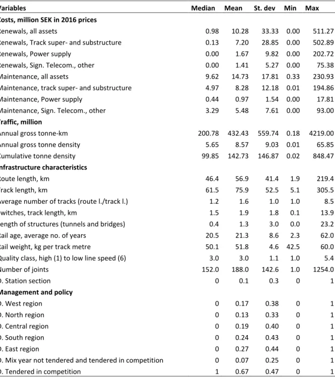
26 Appendix
Table 8: Descriptive statistics, subset of track section data (2003-2016) for analysing infrastructure failures, 2143 observations.
Variables Median Mean St. dev Min Max
Costs, million SEK in 2016 prices
Renewals, all assets 0.98 10.28 33.33 0.00 511.27
Renewals, Track super- and substructure 0.13 7.20 28.85 0.00 502.89
Renewals, Power supply 0.00 1.67 9.82 0.00 202.72
Renewals, Sign. Telecom., other 0.00 1.41 5.27 0.00 75.38
Maintenance, all assets 9.62 14.73 17.81 0.33 230.93
Maintenance, track super- and substructure 4.97 8.28 12.18 0.01 194.86
Maintenance, Power supply 0.44 0.97 1.54 0.00 17.81
Maintenance, Sign. Telecom., other 3.29 5.48 7.61 0.00 93.00
Traffic, million
Annual gross tonne-km 200.78 432.43 559.74 0.18 4219.00
Annual gross tonne density 5.65 8.57 9.03 0.01 65.85
Cumulative tonne density 99.85 142.73 146.87 0.02 848.47
Infrastructure characteristics
Route length, km 46.4 56.9 41.4 1.9 219.4
Track length, km 61.5 75.9 52.5 5.1 305.5
Average number of tracks (route l./track l.) 1.2 1.6 1.0 1.0 8.5
Switches, track length, km 1.5 1.9 1.8 0.1 13.9
Length of structures (tunnels and bridges) 0.4 1.3 3.0 0.0 23.2
Rail age, average no. of years 20.5 21.3 8.6 2.3 62.0
Rail weight, kg per track metre 50.1 51.8 4.6 42.5 60.0
Quality class, high (1) to low line speed (6) 3.0 3.0 1.1 1.0 5.4
Number of joints 152.0 188.0 142.6 1.0 1254.0
D. Station section 0 0.1 0.3 0 1
Management and policy
D. West region 0 0.17 0.38 0 1
D. North region 0 0.13 0.33 0 1
D. Central region 0 0.19 0.40 0 1
D. South region 0 0.24 0.43 0 1
D. East region 0 0.27 0.44 0 1
D. Mix year not tendered and tendered in competition 0 0.07 0.25 0 1