Vibration Analysis of Electronic Unit

(1)

VIBRATION ANALYSIS OF ELECTRONIC

UNIT

VIBRATIONSANALYS AV ELEKTRONIKENHET

Hanna Fahlgren

THESIS 2013

MECHANICAL ENGINEERING

This thesis has been carried out at the School of Engineering in Jönköping in the subject area Mechanical Engineering. The work is a part of the Master of Science program, Product Development and Materials Engineering. The author takes full responsibility for opinions, conclusions and findings presented.

Examiner: Peter Hansbo Supervisor: Rebal Marcos Scope: 30 credits

(2)

Abstract

Components in Airplanes are exposed to vibrations which can cause them to fail due to fatigue if they are not constructed for the extreme environment. High stresses can develop in products during resonance if parts own the same natural frequency. The acceleration induced by one component will couple to the next and give it an even higher acceleration and thus higher inertial displacements and stresses.

Simulations of resonant frequencies and analyses of their couplings were

conducted on electronic units developed by SAAB Electronic Defence Systems in Jönköping. A reinforcement proposal for one of the PCBs in one of their current electronic units was given by the author.

The result of the simulation showed that the first resonant frequency of the investigated PCB and the current chassis was not separated enough, and coupling of their accelerations during resonance occurred. A rib design was developed by the author to increase the natural frequency of the PCB, which eliminated the coupling with the current chassis at its first natural frequency.

A new chassis was being developed by SAAB, which would be produced by casting. Simulations of the casted chassis were also preformed and evaluations with regard to its natural frequency were made. The casted chassis first natural frequency was well separated with the PCB. But the weight ratio between the casted chassis and the PCB would cause high acceleration forces during resonance which would be transmitted to the PCB which is not preferable.

When designing components it is of great importance to know the environment in which they will work. The engineer needs to possess good skills with respect to the phenomena acting on the product in order to find the right input values for simulations. One must also keep in mind that simplifications need to be made so that simulations will not be to complex and therefore evaluation of the result must be preformed to ensure credibility.

Keywords

ANSYS Chassis Coupling

Printed Circuit Board Resonance frequency Simulation

(3)

Summary

Summary

Flygplanskomponenter utsätts för vibrationer som kan leda utmattningsproblem om de inte är konstruerade för den extrema miljö de verkar i. Höga spänningar kan utvecklas i produkter under resonans när komponenter har samma

egenfrekvens. Accelerationer som framkallas av en komponent under resonans kan överföras till en närliggande enhet och ge denna en ännu högre acceleration om deras egenfrekvenser sammanfaller. Detta medför att stora förskjutningar och spänningar i de utsatta komponenterna vilket kan leda till brott och sprickor. Simuleringar av resonansfrekvenser och analyser av deras kopplingar utfördes på elektronikenheter som utvecklats av SAAB Electronic Defence Systems i

Jönköping. Ett förstärkningsförslag för ett av kretskorten i deras nuvarande elektronikenhet togs fram av författaren.

Resultatet av simuleringen visade att den första egenfrekvensen hos det

undersökta kretskortet och det nuvarande chassit inte var tillräckligt separerade, vilket medförde koppling av deras accelerationer vid resonans. Ett

förstärkningsförslag utvecklades av författaren för att öka kretskortets egenfrekvens, vilket eliminerade kopplingen vid det aktuella chassiets första egenfrekvens.

Ett nytt gjutet chassi var under utveckling av SAAB och simuleringar utfördes också av detta chassi. Utvärderingar med avseende på dess naturliga frekvens gjordes. Den första egenfrekvensen hos det gjutna chassit var väl separerat från kretskortets, men viktförhållandet mellan det gjutna chassit och kretskortet skulle medföra höga accelerationskrafter under resonans. De höga krafterna skulle då överföras till kretskortet vilket inte är fördelaktigt.

Vid produktframtagning är det av stor vikt att känna till miljön där

komponenterna ska verka. Ingenjören behöver besitta goda kunskaper om de fenomen som verkar på produkten för kunna ta fram rätt indatavärden för sina simuleringar. Ingenjören måste också veta vilka förenklingar som måste göras så att simuleringar inte blir för komplexa. Förenklingarna medför att utvärderingar av resultatet bör utföras för att säkerställa dess trovärdighet.

(4)

Acknowledgements

I wish to express my sincere gratitude to everyone at the mechanics department at SAAB Electronic Defence Systems in Jönköping. You all made me feel very welcome and a part of your team.

I would also like to give special thanks to my supervisor at SAAB, Rebal Marcos, for helping me with every little problem I had and to Fredrik Kroll, head of the mechanics department, for giving me the opertunity to do the thesis at SAAB. I would also like to gratefully acknowledge my supervisor at Jönköping University, Peter Hansbo, for guiding me through my thesis work.

(5)

Table of Contents

List of Tables

TABLE 1. BOLT SIMULATION TECHNIQUES...22 TABLE 2. CALCULATION OF YOUNG’S MODULUS FROM THE TENSILE

TEST ...27 TABLE 3. COMPARISON BETWEEN THE SIMULATION AND THE PHYSICAL

TEST ...29 TABLE 4. FIRST NATURAL FREQUENCIES OF THE PCBS ...31

(7)

List of Figures

List of Figures

FIGURE 1. ELECTRONIC UNIT ...10

FIGURE 2. SINUS WAVE...13

FIGURE 3. RANDOM VIBRATION. ...14

FIGURE 4. MASS-SPRING SYSTEM...14

FIGURE 5. RESPONSE OF MASS-SPRING SYSTEM ...15

FIGURE 6. STIFFENING RIBS DIRECTLY TO SUPPORT ...20

FIGURE 7. STIFFENING RIBS INDIRECTLY TO SUPPORT ...20

FIGURE 8. ELEMENT SHAPES ...23

FIGURE 9. PULLING IN THE X-DIRECTION ...26

FIGURE 10. PULLING IN THE Y-DIRECTION...27

FIGURE 11. FIRST NATURAL FREQUENCY OF THE CHASSIS. ...30

FIGURE 12. FIRST NATURAL FREQUENCY OF BOTTOM PLATE. ...30

FIGURE 13. FIRST MOOD SHAPE OF THE CONTROLLER MODULE. ...31

FIGURE 14. COUPLING BETWEEN THE CURRENT CHASSIS AND THE CONTROLLER MODULE. ...31

FIGURE 15. COUPLING BETWEEN THE CASTED CHASSIS AND THE CONTROLLER MODULE. ...32

FIGURE 16. ELECTRONIC UNIT WITH PCB BOARD EDGE GUIDES ...34

FIGURE 17. ROBUST ELECTRONIC UNIT WITH MODULAR CLAMSHELL PCB INSERTS ...34

FIGURE 18. CONTROLLER MODULE WITH BOARD EDGE GUIDES. ...35

FIGURE 19. BOARD EDGE GUIDES WITH RIBS, FREQUENCY – RIB THICKNESS. ...36

FIGURE 20. COLLISION OF PARTS WHEN TRYING TO REPOSITION THE CONTROLLER MODULE. ...37

FIGURE 21. FOUR MIDSECTION RIBS. ...38

FIGURE 22. FOUR MIDSECTION RIBS AND SIDE SUPPORT. ...38

FIGURE 23. EXTRA RIBS AT THE POINT OF MAXIMUM EXCITATION. ...38

FIGURE 24. RIB DESIGNS, FREQUENCY – ADDED WEIGHT. ...39

FIGURE 25. RIB DESIGN, INCORPORATING SOLDERED COMPONENTS. ....40

FIGURE 26. RIB DESIGN INCORPORATING COMPONENTS, FREQUENCY – RIB THICKNESS. ...41

(8)

List of Symbols

a Acceleration (m/s²) A Area (m²) B Rib spacing (m) c Damping ((Ns)/m) C Convergence (%) CM Controller module CW Cross wise

EDS Electronic Defence Systems E Young’s modulus (Pa)

f Frequency (Hz) and force with time domain (N) F Force (N)

g Acceleration of gravity (9.81 m/s²)

G Acceleration in gravity units (dimensionless) H PCB Horizontal PCB

HPM High power module

k Stiffness ratio (dimensionless) m Mass (kg)

n Amount of gaps (dimensionless ratio) LW Length wise

p Percentage (%) PCB Printed circuit board RBE Rigid body element

Q Transmissibility (dimensionless ratio) R Frequency ratio (dimensionless ratio) x Displacement (m)

x Velocity (m/s) x

 Acceleration (m/s²)

t Time (s) and thickness (m) v Velocity (m/s) V Volume (m³) w Width (m) W Weight (kg) Greek symbols ε Strain (%) ρ Density (kg/m³) σ Stress (Pa)

(9)

Introduction

1 Introduction

The thesis was carried out at Jönköping University, School of Engineering, in the field of Mechanical Engineering. The work was part of the master program Product Development and Materials Engineering.

The specification of the project was made by SAAB Electronic Defence Systems (SAAB EDS) in Jönköping, where the work was conducted. The author was assigned to carry out vibration analyzes and improvement investigations of an electronic unit. The electronic unit controls the redundant system of flaps and slats in airplanes. The project was created since vibrations in the electronic unit needed to be investigated regarding its impact on fatigue failure.

1.1 Background

SAABs business concept is to constantly develop, adopt and improve new technology to meet the changing customer need. Their high quality products therefore demand thorough investigations to ensure a long life in extreme

environments. The components will be exposed to high temperature changes and vibrations which can cause high stresses and fatigue failure if it is not taken into account. The airplane components are also exposed to high stresses and shock, during flight and landing.

1.1.1 SAAB

SAAB offers world-leading products, services and solutions from military defence to civil security. Their most important markets today are Europe, South Africa, Australia and the US. They have around 13,000 employees and the yearly sale is approximately SEK 24 billion. Their research and development account for about 20% of the sales. SAAB consists of five different business areas, which are [1]:

 Aerodynamics

 Dynamics

 Electronic Defence Systems

 Security and Defence Solutions

 Support and Service

SAAB Electronic Defence Systems develop products in the area of radar and electronic warfare. Their portfolio includes airborne, land based and naval radar, electronic support measures and self-protection systems [1].

(10)

1.1.2 Problem Definition

Today’s airplanes are optimized in regard to weight, which has lead to a decrease of the size of the airplane wings. When the airplane is up in the air at its normal speed, the lifting area of the wing can be decreased. To increase/decrease the wing area the airplane is constructed with slats and flaps. To ensure safe take off and landing, a redundant system is used for this action. The additional system in

SAABs airplanes is run by an electronic motor which is controlled by an electronic unit placed inside the airplane. The electronic unit is exposed to vibrations which could cause some components in the PCBs to fail. Vibrations in the electronics unit therefore needed to be investigated to eliminate further component failures. When the thesis was conducted, the casing of the electronic unit was

manufactured from aluminum sections that were held together by rivets. A new casing manufactured by casting was being developed to reduce manufacturing costs.

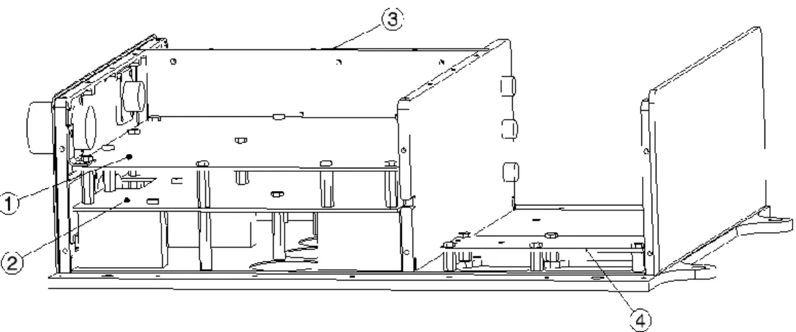
Resonant frequencies and their couplings in the electronic unit were investigated and ways to reduce the displacements of the components were explored. The focus of the simulations was set on the controller module (fig. 1), since it has the most soldered components, where fatigue and tearing could be a problem in lead wires and solder joints.

Figure 1. Electronic Unit. Large PCBs: 1) Controller module, 2) High power module. Small PCBs: 3) Vertical PCB, 4) Horizontal PCB.

(11)

Introduction

1.2 Purpose and Research Questions

The purpose of the thesis was to give the author an opportunity to study failure caused by vibration and to get a deeper knowledge about how to prevent this. The author also learned how to simulate vibrations on a CATIA assembly in ANSYS. The simulations were matched with vibration tests made on the electronic unit in its initial stage to ensure credibility.

The questions to be answered in the report:

 Does coupling at resonance exist between the controller module and the current casing?

 How can displacement of the controller module be reduced during resonance when it is placed in the current casing?

 How does the casted casings current design affect the controller module during vibration?

1.3 Delimitations

A product is only as strong as its weakest link and the weakest link in the electronic unit was estimated to be the controller module since it has the most soldered components. The two smaller PCBs have larger components that are glued well to the PCBs. Since there have not been any noted problems with the glued joints or cracking in the board material, the enforcement proposal will not include these PCBs. The high power module has fewer small components than the controller module and it has more supports holding it in place, which would make it more tolerable. The casings and the other components in the electronic unit, such as the transformer, the bolt in filters and the connectors are far more robust than the PCBs, and they will not be investigated either for further enforcement. Enforcement proposals for the electronic unit with the casted cover will not be investigated since the design is not final. Only investigations of how it affects the controller module will be performed.

(12)

1.4 Outline

Chapter 2 will discuss how vibrations affect components in an airplane with regard to resonant frequencies, transmissibility and displacement. It will also discuss how the design of the chassis can affect the PCB and different fastening technique of PCBs. Methods of decreasing displacements in PCBs, such as dampers and stiffeners, will then be discussed. The procedure of simulation will also be presented.

Chapter 3 will show how the gathering of input parameters and simulations of the electronic units were performed. It will also show the method used to answer the research questions. Analysis of the electronic units will be presented and

enforcement proposals will be stated.

Chapter 4 will show the conclusions of the simulations and evaluate the enforcement proposal. Evaluations of the casted casing will also be presented. Chapter 5 will discuss the method used for finding the answers to the research questions. It will also discuss the simulation result and its reliability. The report will be summed up and proposals for further investigations in the subject will be presented.

(13)

Vibration of Electronic Equipment in an Airplane

2 Vibration of Electronic Equipment in an

Airplane

The vibrations in an airplane are mainly caused by the engines and the aerodynamic buffering. The oscillating movement of the airplane can be

considered as random vibration since the continuous motion does not repeat itself [2].

The vibration frequency spectrum in an airplane varies from 3 Hz to 1000 Hz. The acceleration levels in the vertical direction range from 1 G to 5 G with a frequency range of 100-400 Hz. The frequency range is the same in the horizontal direction as in the vertical direction, but its acceleration level is lower and does not exceed 1 G [2].

2.1 Vibration

Vibration is when an object is subjected to an oscillating motion that causes the body to move back and forth. If the oscillating movement is repeating itself, the vibration is called periodic. The simplest periodic motion is usually represented by a sinus wave (fig. 2). If the continuous motion does not repeat itself, it is called random vibration (fig. 3). The measurement of cycles per second is called Hertz (Hz) and the maximum displacement is called the amplitude of the vibration [2].

Figure 2. Sinus wave [2].

-1.5 -1 -0.5 0 0.5 1 1.5 0 1 2 3 4 5 6 7 8 Time (t) Di sp lace m e n t (y) Period Amplitude

(14)

Figure 3. Random vibration.

To further understand the physics behind vibrations, consider a one degree of freedom undamped system consisting of a mass (m) suspended from a rigid foundation by a spring with stiffness (k) (fig. 4) [2].

Figure 4. Mass-spring system [2].

When the mass is displaced to a given position (x(t)), the force (f(t)) acting on the system can be calculated [2]:

) ( ) ( ) ( 2 2 t kx dt t x d m t f   (eq. 2.1 [2])

If the force subjected to the mass is a simple harmonic excitation with the frequency (ω), it can be described as [2]:

-1.5 -1 -0.5 0 0.5 1 1.5 0 1 2 3 4 5 6 7 8 Time (t) Di sp lace m e n t (y)

(15)

Vibration of Electronic Equipment in an Airplane ) sin( ) (t F t f   _{(eq. 2.2 [2])}

Putting the two equations together, the displacement of the mass can be calculated at a given time increment [2]:

2 ) sin( ) (   m k t F t x   (eq. 2.3 [2]) Large displacements will cause high stresses in the material and it is therefore of great importance to reduce the displacements. Studying the equation 2.3, it can be seen that to reduce the displacement at a given force and frequency, the stiffness needs to be increased and the mass needs to be decreased.

2.2 Resonant Frequency

To understand the resonant frequency phenomena, consider the system in figure 4 and equation 2.1. The equation shows that when the force generated by the

stiffness (kx) is equal to the inertial force generated by the mass element (m2x

) the vibration amplitude builds up cycle by cycle, which makes it go towards infinity, and in practice this causes the system to break (fig. 5) [3].

Figure 5. Response of mass-spring system [3].

0 2 4 6 8 10 0 100 200 300 Frequency (Hz) Resp o n se (kx( t)/F)

(16)

The linearity if the spring in equation 2.1 results in a proportional displacement of the mass to the force applied. The natural frequency of the undamped system can therefore be calculated from the following formula [3]:

m k

n 

 (eq. 2.4 [3])

If a structure has more than one degree of freedom it can have several resonant frequencies showing different patterns of deformation called “modes of

vibration”. The first mode of vibration of a bounded object usually shows the greatest displacement, which causes the highest stresses [2, 3].

In the vibrating environment of an airplane it is of great interest to find the resonant frequencies for the electronic units and their components since they will excite many resonant modes. The electronic support structure must be

dynamically tuned with the electronic components to prevent coincident resonance, which can lead to fatigue failure in a rapid manner [3].

2.3 Transmissibility

The transmissibility (Q) of an object shows its reaction during vibration. The greatest transmissibility occurs at the resonance frequency. The transmissibility can be calculated if the output force (FOut) and the input force (FIn) are known as follows [2]: In Out F F Q

(eq. 2.5 [2])

For a lightly damped system the transmissibility at resonance can be calculated from the stiffness (k), mass (m) and damping (c) using the following formula [2]:

c km

Q  (eq. 2.6 [2])

When the stiffness of an object is increased it is known that the damping is decreased. Equation 2.6 shows that this will lead to an increased transmissibility. Instead if the mass is increased, it is known that the damping will increase which result in a decreased transmissibility [2].

By extensive testing it has been shown that many epoxy fiberglass PCBs, with various edge restrains and closely spaced electronic components, have a

transmissibility at the resonance frequency ( fn) that can be approximated by [2]: n

f

Q (eq. 2.7 [2])

Equation 2.7 shows that when the natural frequency is increased, the transmissibility is also increased.

(17)

2.4 Displacement at Resonance

The displacement in an object is related to the stresses induced in the material and therefore it is of great importance to find the displacement during resonance. When performing vibration tests the usual output data is the frequency (f) and the acceleration force (G), which can be used to calculate the displacement. Consider the system in figure 4, where the displacement of the mass can be represented by the following equation [2]:

) sin(

0 t

x

x  (eq. 2.8 [2])

Deriving the displacement provides the velocity [2]:

) cos( t x dt dx x v   o  (eq. 2.9 [2]) Deriving the velocity provides the acceleration [2]:

) sin( 0 2 2 2 t x dt x d x a   (eq. 2.10 [2])

The maximum acceleration (amax) will occur when sin( t) is equal to 1 [2]: 0

2 max x

a  (eq. 2.11 [2])

Extracting the maximum displacement, while changing the acceleration to

acceleration in gravity units and the frequency from radians/s to cycles/s gives the following calculations [2]: 81 . 9 4 81 . 9 0 2 2 0 2 2 max f x f x g a G    (eq. 2.12 [2]) 2 2 0 4 81 . 9 f G x   (eq. 2.13 [2])

The equation can be developed further by using the knowledge that the input acceleration (Gin) times the transmissibility gives the acceleration at resonance [2]:

2 2 0 4 81 . 9 n in f Q G x   (eq. 2.14 [2])

A PCB can be approximated as a single degree of freedom system when it is vibrating at its first resonant frequency. If the displacement in a PCB is to be calculated, equation 2.7 can be added to equation 2.13 [2]:

n n in n n in f f G f f G x 2 2 2 0 4 81 . 9 4 81 . 9     (eq. 2.15 [2])

Equation 2.15 shows that displacement is increased when the input acceleration force is increased. The equation also shows that the displacement is decreased when the natural frequency is increased.

(18)

2.5 Chassis Design

The chassis of the electronic unit should work as a protection and a support for the PCB. It is of great importance to find the natural frequency of the casing and the PCB and to compare these. If the natural frequency of the chassis and the PCB are the same or close to each other, it can lead to coupling of their transmissibilities and cause the electronic unit to vibrate at extreme levels. The octave rule should therefore be used when designing the chassis. The octave rule states that the frequency of the chassis and the PCBs should be separated by at least a ratio of two [2].

There are two different octave rules called the forward and the reverse octave rule. The forward octave rule (eq. 2.16) states that the PCB ( fPCB) should be have a natural frequency twice as high as the chassis ( fcha). The reverse octave rule (eq. 2.17) says that the chassis should have a natural frequency twice as high as the PCB. 2   cha PCB f f f R (eq. 2.16 [2]) 5 . 0   cha PCB r f f R (eq. 2.17 [2])

The forward octave rule works for all kind of electronic units, but the reverse octave rule has some limitations. For the reverse octave rule to work the weight ratio between the chassis (WCha) and the PCB (WPCB) has to be less than 0.10 [2]:

10 . 0  Cha PCB W W (eq. 2.18 [2])

If the weight ratio is higher than the recommended level, it can cause high acceleration G levels, with a reduced PCB fatigue life.

2.6 Fasteners

If a PCB is subjected to a severe shock and vibration environment, as in an airplane, a loosely fastened PCB will develop high acceleration loads, which will lead to high deflection and stresses in components mounted on the PCB [2]. There exist many different types of fastening techniques such as screws, nuts, rivets, clips and board edge guides. The methods used for ease of installation and low cost are usually not satisfactory for severe shock and vibration environments [2].

(19)

A board edge guide that grips the edge firmly is desirable since this can reduce deflection due to edge rotation and translation, which in turn will increase the natural frequency. Due to friction and relative motion between the PCB and the edge guide, more energy will be dissipated during vibration, which will reduce the transmissibility during resonance. Board edge guides are in general more costly than other fastening techniques because of the high tolerances needed for a tight fit and the complication of attaching the PCB to the connectors [2].

Bolted joints will experience a substantial amount of relative motion during resonance. The relative motion may add damping to the system and reduce the transmissibility and the natural frequency of the structure. When bolts are used to fasten the PCB an efficient factor can be estimated. The bolted efficiency factor is the bolts ability to hold to membranes together during vibration. For a welded connection it is 100%, for a joint that has no connection it is 0% and for regular screws it is usually about 25% [2].

2.7 Damping

When damping electronic equipment one must keep in mind to provide sway space to ensure that objects do not collide. Connecting wires and couplings must be designed to guarantee that the damped parts can move without tearing the wires/couplings or causing them to fail due to fatigue. The design of the damping equipment must therefore consider the specific environment where the equipment is installed. If space is an issue, like in most airplanes, it might be more practical to use hard mounts [2].

For low natural frequencies below 50 Hz, dampers can be quite efficient. But for natural frequencies above 100 Hz, dampers are not very effective in reducing the transmissibility. Most dampers are also rather sensitive to high temperature changes because of the polymer materials that are most commonly used. At a low temperature, the damper can become too stiff and at high temperatures, they can become too soft. One must also keep in mind that a good vibration isolator is often a poor shock absorber and vice versa [2].

2.8 Stiffeners

Ribs are often mounted on PCBs to increase the resonant frequency and reduce board deflection during resonance. For high frequencies they often work better at reducing the transmissibility than dampers. The reduced board deflection will reduce the stresses in the electronic component lead wires [2].

Ribs are mostly fabricated from steel, aluminum or epoxy fiberglass. Caution must be taken when using metal ribs since short circuits can occur across exposed electrical printed circuit strips. Ribs can be bolted, riveted, soldered, cemented, welded, or cast integrated with heat-sink plates. They can be attached around the edges and/or on the surface in several directions depending on the type of displacement prevented [2].

(20)

If the ribs are not designed properly, they will not increase the stiffness of the PCB. The ribs should be placed so that they carry the load directly to the support (fig. 6), if this is not possible, a secondary membrane should be added to carry the load to the support (fig. 7) [2].

Figure 6. Stiffening ribs directly to support [2].

Figure 7. Stiffening ribs indirectly to support [2].

To estimate the spacing (B) of the stiffening ribs the thickness of the PCB (t) can be used as follows [4]:

t

B30 (eq. 2.19 [4])

The stiffness of the material used for the ribs should be at least equal or greater than the stiffness of the PCB [4].

2.9 Simulation Technique

The main areas to take into consideration when building the simulation are the properties of the PCB, chassis modeling and boundary conditions. It is of good practice to model the chassis of the electronic unit, since neglecting this can severally affect the accuracy of the simulation. When the aim of the simulation is to find the resonant frequencies of the unit, a “smearing technique” can be used to add the properties to the PCB [5].

(21)

2.9.1 PCB Simulation

A smearing technique models a highly simplified representation of the PCB by adding summarized values of the PCB to the base board. There are different levels of accuracy that can be used, such as global mass smearing, global mass/stiffness smearing and local smearing. Global mass smearing adds extra mass to the base board while global mass/stiffness smearing also adds the physically tested stiffness of the base board. Local smearing on the other hand, adds extra stiffness and mass to local areas of the base board [6].

To find the properties needed for the simulations physical tests can be made on parts of the PCB or the whole, depending on the technique used. The Young’s modulus can be calculated from a bending test and the density can be calculated from the mass and the dimensions [6].

2.9.2 Bolted Joint Simulation

When attaching the PCB to the chassis, constraints should be carefully selected. The translational displacement can in most cases be simulated by a fixed

constraint, but the rotational displacement needs rotational spring elements since all fixing methods will display some flexibility. The stiffness of the spring elements can be found using a trial and error approach, tuning the resonant frequency of the model to that of the vibration tested prototype [5].

There are different ways of modeling bolts in a simulation, such as: no bolt, coupled bolt, RBE bolt, spider beam bolt, hybrid bolt and solid bolt. The table below describes the modeling technique and its pros and cons (tab.1) [7].

(22)

Table 1. Bolt simulation techniques [7]

Technique Pro Con

No bolt The bolt and nut are

replaced with a pressure on the washer surface.

Simple approach which lead to short computation time.

The load is not transferred through the bolt and the bolt stiffness is not taken into account.

Coupled bolt Line elements

represents the stud and coupled nodes represents the head/nut.

Relatively simple approach with few elements.

The tensile lads can be transferred through coupled nodes.

Ease in extracting results.

Bending loads are not transferred. Head/nut

temperatures are not taken into account.

RBE bolt Line elements are

used to represent the stud and rigid body elements are used to represent the

head/nut.

Relatively few elements as in the coupled bolt. Tensile, bending and thermal loads can be transferred through RBE nodes.

Head/nut

temperature is not taken into account.

Spider beam bolt

The head and nut are represented by line elements in a web-like fashion. The stud is represented by line elements.

Less elements than hybrid and solid bolt. Tensile, bending and thermal loads can be transferred through the spider elements.

Extra work required to simulate head/nut stiffness.

Hybrid bolt The head and nut are

simulated by solid elements and the stud is simulated by line elements.

Better accuracy in comparison to previous simulation techniques. Tensile, bending and thermal loads can be transferred through the line elements.

Full stress distribution can be calculated in head and nut.

Simple stud section which result in shorter computational time in comparison to solid bolt. Ease in extracting results.

Stress distribution in the stud is not accounted for. Coupling of line elements to stud is required which ads model complexity.

Solid bolt The head, nut and

stud are modeled as solids.

Gives the most accurate results.

Tensile, bending and thermal loads can be transferred.

Full stress distribution in head, nut and stud can be computed.

The computational time is greater than in the previous simulations. Contact elements are required between head/nut to the flanges.

(23)

When modeling bolts one must take in consideration the conditions under which the bolt will be used such as compression, tension and shear stresses or a

combination of these. This is important since the boundary conditions and simulation technique affects the output data, the computational time, and the accuracy of the result [7, 8].

2.9.3 Boundary Conditions and Constraints

When performing a modal simulation in ANSYS, only linear constrains can be used, such as bounded and no separation. Other constraints such as frictionless, rough and frictional cannot be used since these constraints are nonlinear. The nonlinearity of these constraints comes from the fact that the contact surfaces can be separated during the simulation. If nonlinear constraints are used, they will be transformed to linear constraints by ANSYS during the simulation [9, 10].

The bounded constraint does not allow any sliding or separation between faces or edges and the contact areas can therefore be considered as glued. The no

separation boundary condition is similar to the bounded constraint, with the exception that the contact areas can slide a small amount in relation to each other, but the contact areas cannot separate [9].

2.9.4 Mesh

There exists several different element types that can be used when meshing an object. When a three dimensional model is used, tetrahedral, pyramid, wedge or hexahedral elements can be used (fig. 8). The tetrahedrally shaped element is a good choice for complex shapes, but it causes a higher apparent (numerical) stiffness in bending than the hexahedral element [10].

(24)

The shape of the elements should be as close to the shape of an equilateral triangle or square with the aspect ratio as close to one as possible to avoid errors. It is tolerable to have some bad elements, as long as they are located in regions of low stress gradients [11].

The sizes of the elements are also of great importance when performing a simulation, since a too coarse mesh can produce results that are not reliable. To ensure that the mesh used is good enough, a mesh refinement study should be preformed. To ensure a good mesh the percentual convergence should be below 5% when computing mode frequencies according to good practice. Using a too fine mesh will lead to high computational time which is not economic in regard to the usage of resources [9].

If the shape of the object to be meshed is complicated and there is a risk of stress concentration a fine mesh should be used. To improve the mesh even further and to avoid the risk of creating a mesh with too many elements, higher order or quadratic shape functions can be used. A higher order or quadratic shape functions creates more nodes where the variables can be calculated [11].

(25)

Simulation of the Electronic Unit

3 Simulation of the Electronic Unit

The simulations of the electronic unit were computed using ANSYS Workbench, where modal analysis was used to extract the natural frequencies.

To get the input data for the simulations, tensile tests were made on the controller module to find its elastic modulus. The large components off the electronic units were weighed and their densities were calculated.

A mesh refinement study was made on all components in the old and the new electronic unit also including the casted and the casing with assembled sections. Before the simulation process could start, some components had to be redesigned by simplifying their shapes to make the simulation run faster. The simplifications made were to eliminate all small components on the PCBs, adding the extra mass using the global mass smearing method. All connecting wires, component lead wires, washers and components attached to the heat sinks were also removed. The shape of the screws, the chassis, the chokes on the vertical PCB, the transformer, the connectors and the bolt in filters were simplified, while still holding their main features.

ANSYS generates bounded constraints at all contact surfaces, these constraints were therefore removed from all components that were connected with screws. The bounded constraints were held at the screws contact surfaces to simulate the contact force and friction. The parts in the electronic unit that were glued were also bounded at their contact surfaces. The electronic unit was constrained in the four base holes to simulate the electronic unit being bolted to a rigid foundation. The electronic unit was meshed using the data from the mesh refinement study. Tetrahedral elements were used for the more complex parts such as the chassis and hexahedra elements were used for the parts with simple geometries such as the square capacitors.

To be able to compare the results from the physical test made by SAAB, the old electronic unit had to first be modeled. The electronic unit was then modeled again using the current design and the casted cover. The components used in the different simulations can be found in appendix A.

Different enforcement proposals were also investigated and there pros and cons where weighted against each other to obtain the final design. The final design was then simulated and the results were gathered for the comparison between the current and the enforced electronic unit.

(26)

3.1 Physical Tests

The indata values needed for the simulations was Young’s modulus and density for the components in the electronic unit. Physical tests and calculations where preformed to find these values.

3.1.1 Young’s Modulus of PCBs

Three controller modules were used for the tensile test and two of the controller modules were cut in half at opposite directions. To be able to attach the PCBs to the tensile test machine, some components had to be removed around the

gripping area to ensure good contact.

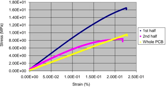
The specimens were not pulled to their rupture point since only the modulus of elasticity was needed. The stress strain curves from the test can be found in figure 9 and 10.

Figure 9. Pulling along the x-direction

0.00E+00 2.00E+00 4.00E+00 6.00E+00 8.00E+00 1.00E+01 1.20E+01 1.40E+01 1.60E+01 1.80E+01

0.00E+00 5.00E-02 1.00E-01 1.50E-01 2.00E-01 2.50E-01 Strain (%) 1st half 2nd half Whole PCB S tr e s s (M P a )

(27)

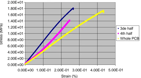
Figure 10. Pulling along the y-direction

Two points on the curves straightest parts were used to calculate the elastic modulus (E) and the result from the calculations (eq. 3.1) is shown in table 2.

2 1 2 1        E (eq. 3.1)

Table 2. Calculation of Young’s modulus from the tensile test

The main material of the PCB is epoxy fiber glass (FR-4) which is a woven fiber glass that has a theoretical Young’s modulus of 24.1 GPa in the LW direction and 20.7 GPa in the CW direction. The test result shows a much smaller elastic

modulus of 42-82 MPa in the LW direction (tab.2). The test values were therefore discarded and not used for the simulations.

Since the test values of the PCBs were discarded more detailed models had to be computed, also taking into account the copper films. The thickness of the copper film and the percentage of copper in the different layers were considered in the calculations (appx B).

Part of PCB Stress 1 (MPa) Stress 2 (MPa) Strain 1 (%) Strain 2 (%) Young's Modulus (MPa)

1st half X-direction 8.2 1.6 0.094 0.014 82

2nd half X-direction 5.2 1.9 0.090 0.025 51

Whole X-direction 8.0 2.4 0.19 0.052 42

3de half Y-direction 16 3.0 0.22 0.037 69

4th half Y-direction 14 6.8 0.24 0.13 65 Whole Y-direction 11 3.0 0.26 0.067 42 0.00E+00 2.00E+00 4.00E+00 6.00E+00 8.00E+00 1.00E+01 1.20E+01 1.40E+01 1.60E+01 1.80E+01 2.00E+01

0.00E+00 1.00E-01 2.00E-01 3.00E-01 4.00E-01 5.00E-01 Strain (%) 3de half 4th half Whole PCB St re ss (MPa )

(28)

3.1.2 Densities of Composite Components

The components that consisted of several different materials were weighed on a scale that could receive values from 1g and their volumes were measured in CATIA. Some of these components could not be removed from the electronic unit and their weights were therefore obtained from the suppliers’ data sheets. The density calculations can be seen in appendix C.

3.2 Mesh Refinement Study

To ensure that the result computed was accurate, a mesh refinement study was performed on all of the parts in the simulation (appx. D). Since parts were modeled separately, the boundary conditions used were simulating their

attachment in the electronic unit, but not taking into account the flexibility of the connections or the flexible support from connected parts. The results of the modal frequencies are therefore not fully reliable and can thus only be used as a rough comparison with the actual results. The two last frequency results were compared and the percentage of the convergence was computed which aimed at a convergence of at least 5% (appx. E).

The mesh from the mesh refinement study was added to the electronic unit. When studying the mesh, it could be seen that the mesh of the envelope, bottom plate, the casted casing and its top had long thin elements around the screw holes. The mesh of these parts was therefore changed to obtain evenly shaped elements. The simulation was run, but the high number of elements in the simulation caused it to fail. The author therefore decided to use the mesh from the mesh refinement study on the parts of most interest. These parts and their element sizes are shown in appendix F.

The rest of the parts in the simulation were assigned the automatic generated fine mesh by ANSYS. These parts are also shown in appendix F, together with the error of the natural frequency received from the coarser mesh. The changed mesh will add extra stiffness to the parts outside of the limit and also extra stiffness to their couplings.

(29)

3.3 Simulation of the Old Electronic Unit

The material database in ANSYS contains the most common materials such as steel, aluminum and copper, which were used in the simulation. Some more rare materials which was needed for the simulation, was not included in the database and therefore needed to be added to the program. Properties other from the density needed for the simulation was Young’s modulus (appx. G). The capacitors, the chokes, the bolt in filter, the connectors and the transformer where composed from several materials. The chokes, the connectors, the bolt in filter and the transformer are represented by the Young’s modulus of the main material in the component. The author was in contact with the supplier of the capacitors, but the material composition was not received. The Young’s modulus of the capacitors was therefore calculated from the density of the component and the respective densities of the two main materials.

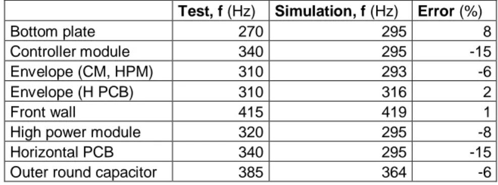
The complete electronic unit was simulated, and the oscillations of the

components were compared to the physical vibration tests made by SAAB (tab. 3). The frequency at which the first accelerations occurred in the physical test was compared to the first oscillation of the tested measuring point in the simulation. Account was also taken of the direction of the excitation in the simulation since the sensors in the test only measured in a specified direction.

Table 3. Comparison between the simulation and the physical test

Test, f (Hz) Simulation, f (Hz) Error (%)

Bottom plate 270 295 8

Controller module 340 295 -15

Envelope (CM, HPM) 310 293 -6

Envelope (H PCB) 310 316 2

Front wall 415 419 1

High power module 320 295 -8

Horizontal PCB 340 295 -15

(30)

3.4 Simulation of the Current Electronic Unit

The input data for the simulation of the current electronic unit was held the same as for the old electronic unit with the exception of adding the new components and their properties (appx. H).

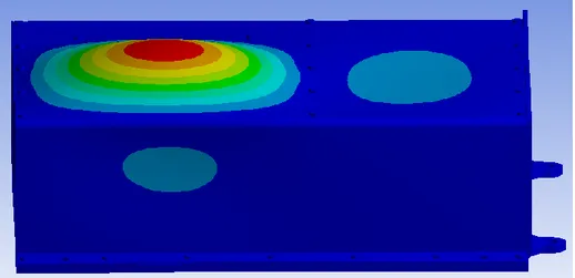
When computing the first simulation of the new electronic unit, only the chassis was simulated. This simulation showed the first natural frequency at 309Hz with the maximum excitation in the envelope above the controller module, transmitting the vibrations to the rest of the chassis (fig. 11). The bottom plate had its first natural frequency at 549Hz, which made the whole chassis oscillate (fig. 12).

Figure 11. First natural frequency of the chassis.

(31)

The PCBs were then simulated separately with their larger components and their first natural frequencies can be found in table 4.

Table 4. First natural frequencies of the PCBs

Part 1st frequency (Hz)

Controller module 399 High power module 367

Horizontal PCB 356

Vertical PCB 169

The maximum excitation of the controller module was found in the area where the support pad and plate is located (fig. 13).

Figure 13. First mood shape of the controller module.

In the next simulation all components of the new electronic unit was added. The coupling of the natural frequencies was investigated between the chassis and the controller module and the first coupling was found at 286Hz (fig. 14). In the physical test made by SAAB, the first coupling mood of the bottom plate and the controller module was found at 295Hz.

(32)

3.5 Simulation of the Casted Cover Electronic Unit

When simulating the casted cover electronic unit, the same input data as for the current electronic unit was used, with exception of the removal of the controller module ground plate. The casted aluminum cover was also added using the same properties for the material as in the previous simulations.

The chassis was first simulated by itself giving it a first natural frequency of 305Hz, which only showed an excitation in the top cover. There was no coupling of the casted casing and the top cover until the frequency 869Hz.

The total casted cover electronic unit was then simulated, which showed the first coupled frequency between the top casted cover and the controller module at 408Hz (fig.15). Coupling between the controller module and the high power module was found at 372Hz. The simulation was run till 438Hz and no coupling between the casted casing and the controller module was found.

(33)

3.6 Enforcement Proposals and Simulation

The simulations show that the natural frequency of the current electronic unit chassis is close to the natural frequencies of the controller module, which is not desirable, since this lead to coupling at resonance which was also found in the simulations. Their natural frequencies need to be separated by at least an octave. The weight ratio will therefore be calculated to find which octave rule to use for the enforcement. The input data for the calculation can be found in appendix I. The weight ratio was then calculated from the weight of the PCBs (WPCB), the casted chassis (WCast) and the sheet metal chassis (WSheet) as follows:

40 . 0 18 . 3 29 . 1 _  Cast PCB W W (eq. 3.1) 53 . 0 41 . 2 29 . 1 _  Sheet PCB W W (eq. 3.2) As can be seen from the calculations, the weight ratio is higher than 0.10 and therefore the reverse octave rule is not valid. The forward octave rule was therefore used for the enforcement proposal.

There are some different ways of increasing the natural frequency of the PCBs, such as improving the boundary constrains or making the PCBs stiffer. The PCB boundary constraints could be improved using close board edge guides or more screws and spacers. To improve the stiffness of the PCBs the thickness could be increased or ribs could be added.

Another way of reducing the acceleration of the PCBs at the coupled resonance could be to add dampers to the spacers and the section wall that connect the PCBs to the chassis. But the natural frequencies of the PCBs are above 100 Hz and therefore a damping solution is not preferable. Dampers will also reduce the natural frequencies of the PCBs and in this case the aim is to increase the natural frequency. The damping solution was therefore rejected by the author.

3.6.1 Bench Marking

To find clamping solutions for the PCBs bench marking was used. Electronic units from Esterline Technologies Corporation and Schroff/Pentair Technical Products were investigated.

Figure 16 shows an electronic unit used for power distribution and control in airplanes, helicopters, military equipment, boats and industries. It has PCB board edge guides made from lightweight metal, which reduces weight and makes maintenance easier [12].

(34)

Figure 16. Electronic unit with PCB board edge guides [12].

Figure 17 shows a robust embedded computing system used in military, aerospace and railway sectors. The chassis is produced from aluminum with attached heat sinks. The clamshells are locked into position by card locks, which conduct the heat from the PCB to the chassis in an effective manner. The clamshells and card locks allow easy maintenance in the field, which is required by the US military [13].

(35)

3.6.2 Enforcement Design

The enforcement alternatives stated in 3.6 where evaluated in regard to their efficiency in increasing the stiffness ratio and their probability of being

implemented. The alternative of increasing the number of screws and spacers was rejected by the author, since this solution had already been investigated by SAAB and they had decided to not go any further. The alternative of increasing the board thickness was also rejected by the author, since it is not an effective way of increasing the natural frequency. Adding extra material will make the board stiffer but it will not increase the stiffness ratio. The author decided to investigate the enforcement alternative of adding board edge guides and/or stiffening ribs to the current electronic unit since this will increase the stiffness ratio. The support plate and the support pad were removed from the electronic unit since the aim of the enforcement design was to find a stiffening solution for the controller module.

Board Edge Guide Design

Simple board edge guides where designed from aluminum, not taking into account the locking mechanism that would prevent the board from sliding out of the chassis guide (fig. 18). The controller module was bounded into place using the no separation boundary constraints at the contact surfaces. The board was also

bounded at the outer edges to prevent it from sliding out of the chassis guide.

Figure 18. Controller module with board edge guides.

The simulation showed that the board edge guides where not enough to give the controller module a reasonable first natural frequency. Ribs were therefore added to the controller module to increase the natural frequency. Equation 2.17 was used to find proper spacing between the ribs.

mm t

B30 30*260 (eq. 3.3)

The number of ribs (n) was calculated using the width of the board (w).

3 60 / 180 /   w B n (eq. 3.4)

The simulation was first run setting the width of the ribs to 8mm, changing the thickness of the ribs to approach the aimed frequency of 618Hz (fig. 19).

(36)

Figure 19. Board edge guides with ribs, frequency – rib thickness. Figure 19 shows linearity up to 745Hz where a dip occurs. The dip can be explained by the change of mode shape at this frequency. Since the relation between the frequency and the rib thickness seems linear at the aimed frequency, the linearity assumption can be used to calculate the thickness of the ribs.

mm df f f dt t a rib 4.86 5 ) 162 912 ( ) 162 618 )( 0 8 ( ) ( ₀         (eq. 3.5) 0 100 200 300 400 500 600 700 800 900 1000 0 1 2 3 4 5 6 7 8 9 Rib thickness (mm) Fre quenc y (Hz)

(37)

When trying to implement the board edge guide design in the electronic unit it was found that it was not possible to use the idea. The board edge guides would collide with the connectors if the controller module would be placed in its current position. The position of the controller module could not be altered since there were components connecting the controller module with the high power module. The high power module could not be repositioned either, since it was connected to the heat sinks. The repositioning of the controller module would therefore affect the heat sinks, which would have to be redesigned. The round capacitors, which were connected to the high power module, would also collide with the bottom plate and would have to be replaced with similar smaller components. The above mentioned collisions are illustrated in figure 20 below. The board edge guides where discarded as a solution to the enforcement problem of the electronic unit since it could not be fitted in the current design.

Figure 20. Collision of parts when trying to reposition the controller module.

Rib Placement with Spacer Connections

Since the board edge guides where discarded, a rib design using the spacers that are currently holding the controller module in place where used. Three different designs of rib placement were investigated with aluminum ribs cemented to the boards. The first design had four ribs crossing the midsection in two directions carrying the load directly to the spacers (fig. 21). The second design hade the same four ribs, but ribs along the sides were also added (fig. 22). The third design was set the same as the second design also adding two ribs crossing each other at the point of maximum excitation (fig. 23). The designs did not take into account the components mounted on the back of the controller module. If any of the designs were to be used, the components on the back of the controller module would have to be repositioned.

(38)

Figure 21. Four midsection ribs.

Figure 22. Four midsection ribs and side support.

(39)

The first natural frequency for different thicknesses of the grids was simulated and the result of the simulations is shown in figure 24. As can be seen from the

diagram the relation between the thickness and the frequency is linear for the second and the third design. The nonlinearity of the first design comes from a change in the mode shape, where two of the edges start oscillating instead of the midsection.

Figure 24. Rib designs, frequency – added weight.

Since all designs are linear at the aimed frequency of 618 Hz, the linearity assumption can be used for the thickness calculations. Using the linearity, the thickness (t) of the aimed frequency ( fa) can be calculated as follows.

mm df f f dt t a 2 55 . 1 ) 399 1107 ( ) 399 618 )( 0 5 ( ) ( ₀ 1         (eq. 3.6) mm df f f dt t a ₁_.₀₇ ₂ ) 399 1426 ( ) 399 618 )( 0 5 ( ) ( ₀ 2 _        (eq. 3.7) mm df f f dt t a ₀_.₈₈ ₁ ) 399 1647 ( ) 399 618 )( 0 5 ( ) ( ₀ 3 _        (eq. 3.8)

The weight was then calculated using the rib designs and the thicknesses from calculations 4.6-4.8. The weight of the first design was 27g, the second design had a weight of 54g and the third designs weight was 32g.

0 200 400 600 800 1000 1200 1400 1600 1800 0 50 100 150 200 Added weight (g) Fre quenc y (Hz) _{Design 1} Design 2 Design 3

(40)

Incorporating Components in Rib Design

The first rib designs with spacer connections, previously presented in the end of chapter 3.6.2 did not take into account the components mounted on the back of the controller module. If the placement of the components could not be altered, a rib design would have to be found incorporating the placement of the

components. A new rib design was therefore developed by the author (fig. 25). The first rib design with spacer connections was used as a reference when modeling the component incorporated rib design. The reason for choosing this design as a reference was that it had the lowest weight.

(41)

The first natural frequency was found for different thicknesses of the grid. The relation between the thickness and the first natural frequency is linear to 1187Hz where the mode shape changes, as can be seen from the diagram (fig. 26).

Figure 26. Rib design incorporating components, frequency – rib thickness. The thickness of the ribs (trib) was than calculated using the linearity assumption:

mm df f f dt t a rib 1.11 2 ) 399 1087 ( ) 399 618 )( 0 5 . 3 ( ) ( ₀         (eq. 3.9)

The incorporated component rib design was inserted in the current electronic unit and a simulation was run. The simulation ran till 416 Hz and showed one

excitation of the controller module at 310Hz when the chassis and the high power module started to oscillate. The reason for the oscillation could have to come from the fact that the controller module has a higher natural frequency than the chassis that is attached to the controller module through the spacers. The first natural frequency of the controller module was therefore used to calculate the new minimum thickness of the ribs.

mm df f f dt t_rib a 1.71 2 ) 399 1087 ( ) 399 736 )( 0 5 . 3 ( ) ( ₀         (eq. 3.10)

The calculations gave the same minimum thickness of the ribs that had already been proven to fail. The aimed-for frequency used for the calculations in 3.9 belonged to the envelope that transmitted the vibrations to the bottom plate. The author decided to use the first natural frequency of the bottom plate instead, which was 549Hz. 0 200 400 600 800 1000 1200 1400 0 1 2 3 4 5 6 Rib thickness (mm) Fre qe uncy (Hz)

(42)

mm df f f dt t_rib a 3.56 4 ) 399 1087 ( ) 399 1098 )( 0 5 . 3 ( ) ( ₀         (eq. 3.11)

The new simulation was run till 408Hz and showed no coupling at the resonant frequencies. The bottom plate had its first natural frequency at 310 Hz, but as can be seen in figure 27, there is no excitation of the controller module, it is merely following the movement of the bottom plate.

Figure 27. First natural frequency of bottom plate.

The weight of the grid was calculated from the thickness of the ribs and found to be 68g. With the removal of the support plate and material at the spacers, the additional weight of the enforcement solution was calculated to 19g.

(43)

Findings and Analysis

4 Findings and Analysis

Coupling between the controller module and the current design was found in chapter 3.4. To prevent the coupling at resonance different stiffening proposals for the controller module was investigated by the author in chapter 3.6. The casted casing was also evaluated with regard to its robustness during vibrations.

4.1 Evaluation of Enforcement Proposal

The component incorporated rib design modeled in the previous chapter was selected as the best stiffening solution by the author. The reason for selecting the design was that it had the most potential of being implemented in the current electronic unit.

A simulation of the current electronic unit was made with the component incorporated rib design added. The simulation of the current electronic unit was compared with the simulation of the same electronic unit with the added

enforcement. The comparison showed that the enforcement made the coupling occur at a higher frequency. The separation of the first natural frequencies of the chassis and the controller module will result in lower acceleration forces acting on the controller module during the natural frequency of the chassis. A higher natural frequency of the controller module will also result in smaller displacements in the controller module at its first natural frequency. Lower acceleration levels acting on the controller module and smaller inertial displacements will result in lower

stresses in the controller module and its components.

But account must be taken to the change in mode shape of the controller module that accrues at 1187 Hz. The new mode shape has its maximum excitation along one of the sides of the PCB. These components might therefore be exposed to higher acceleration levels than what they are exposed to in the current design. If this is the case, an extra board could be added along the sides to prevent the mode shape from changing.

(44)

4.2 Vibration Evaluation of the Casted Electronic Unit

The simulation of the casted cover showed no coupling of the casted casing and the controller module around the first natural frequency of the controller module, which was expected by the author. The author believes that this is caused by the high natural frequency of the casted casing that was found at 869Hz. The reverse octave rule was used to calculate the ratio (Rr) between the casted casing and the controller modules first natural frequencies.

46 . 0 869 399 _   cha PCB r f f R (eq. 4.1)

When using the reverse octave rule, the ratio should be below 0.5, which is fulfilled by the casted electronic unit. For safe use of the octave rule, the weight ratio between the chassis and the PCB should be below 0.1. But the weight ratio calculated in chapter 3.6 gave a value of 0.4, which is above the limit. This will lead to high acceleration levels when the vibrations reach the first natural frequency of the chassis.

(45)

Discussion and Conclusions

5 Discussion and Conclusions

The method used for answering the research questions was investigated and the input data for the simulation was thoroughly investigated by the author. The result from the work was compared to Stenberg’s conclusion in his book, Vibration Analysis of Electronic Equipment [2]. Recommendations for further work on the subject were then presented.

5.1 Discussion of Method

To find out whether coupling at resonance exist and how this can be prevented, simulations using ANSYS Workbench on CATIA products where performed. The simulations also answered how the casted casings design affects the controller module. During the process of finding the answers to the research questions, the author learned how failure caused by vibration can be created and she got a deeper knowledge about how this can be prevented.

To receive the Young’s modulus of the controller module a physical test was made. The result gave a stiffness which was almost 500 times smaller than the Young’s modulus of the main PCB material in the electronic unit. The bad results from the tensile test might have been a result of sliding of the PCB in the

measurement equipment. If the PCB was not properly clamped to the equipment it could also have resulted in an uneven distribution of forces in the material which could be another explanation too the wrong test value. A better way of finding the stiffness of the controller module would have been to use a bending test.

The calculations made to find the stiffness of the controller module did not take into account the distribution of copper in the PCBs, which might have affected the mode shapes of the controller module. The smaller components soldered to the surfaces of the PCBs where not considered in the calculations either. These components are mostly stiffer than the PCBs, which could have been the reason for the slightly lower first natural frequency of the PCBs in comparison to the physical tests made by SAAB. Incorporating the small components attached to the PCBs in the simulation would not have been an alternative since this would have made the simulation too complex to run.

The calculated stiffness of the other composite components holds some inaccuracy since it does not take into account the distribution of the different materials in the components. Including the material distribution in the

components would however have made the simulation too complex, and it was therefore not an alternative for the simulations. The input data received from the supplier was not checked by the author and could have contained values that were not correct. A thorough examination of the components, where the components would have been taken apart could have been an alternative, but this would have required a lot of precision and time and was therefore not an option.

(46)

The mesh used for the simulation most probably added numerical stiffness to the simulation. If the mesh from the mesh refinement study could have been used, this would have given a more accurate result. This limitation had to be made to ensure that the simulation was able to run.

The constraints used when bounding the components in the simulation showed some limitation, since only fixed and no separation boundary constraints were available for modal simulation. In reality, friction and contact pressure also affect the connections. At low acceleration levels the bounded constraint can represent the friction and contact pressure, but at high acceleration levels on the

components they would separate in reality, which the simulation constraints do not allow. For high acceleration levels the result of the simulation might therefore not be as reliable.

The author did not use springs in the attachment of the screws in the simulation since she did not find the input values for the composite components to be fully reliable. Trying different stiffness of the springs could have yielded a result much closer to the tests made by SAAB. However, the reliability of the spring stiffness would have been poor, since this would merely cover up the error from the composite components.

Despite all uncertainties in the simulations, they showed that couplings exist, which was supported by the physical tests made by SAAB, making the result reliable. The reliability of the enforcement solution and the simulation of the casted electronic unit were ensured by the usage of the same method as for the current electronic unit, which had been proven to be reliable. The validity of the result was therefore considered to have been meet by the author.