Evaluation of water spray as a boost function for a cooling system

(1)

M¨

alardalen University

School of Innovation, Design and Engineering

V¨

aster˚

as, Sweden

Thesis for the Degree of Bachelor of Science in Engineering

-Aeronautical Engineering 15.0 credits

EVALUATION OF WATER SPRAY AS A

BOOST FUNCTION FOR A COOLING

SYSTEM

Mohammad AL-Jumaily

may12001@student.mdh.se

Robin Lindfors Lindell

rll12001@student.mdh.se

Examiner: H˚

akan Forsberg

M¨alardalen University, V¨aster˚as, Sweden

Supervisor: Jacob Brynolf

M¨alardalen University, V¨aster˚as, Sweden

Company supervisor: Harald Pettersson

SAAB, Arboga, Sweden

(2)

(3)

Preface

This report is the result of a thesis within the Aeronautical Engineering Program 180 credits at Mälardalen University, Väster˚as. This thesis has been carried out in cooperation with SAAB, Support and Services, Sensor and Test. It has been performed through the spring of 2015 at SAAB, Arboga. Supervisor at Mälardalen University was Jacob Brynolf and the supervisor at SAAB was Harald Pettersson.

V¨aster˚as, May 2015

Mohammad AL-Jumaily Robin Lindfors Lindell

(4)

(5)

Abstract

Many avionic components emit heat at operation. Unhandled this may affect their perfor-mance. The performance of an avionic component is affected by its operational working temperature and ambient temperature. The components need to be cooled to maintain a proper working temperature. Cooling of the components during normal conditions is satis-factory. Problem occurs when ambient temperature is high, which may reduce the cooling capacity below the required levels. The main task in this thesis was to investigate the pos-sibilities to improve the cooling capacity by inducing water spray in the cooling airstream. The spray uses heat from the heat exchanger in order to vaporize. This results in a lower return temperature of the cooling water from the heat exchanger, which is also defined as the working temperature. The focus of this thesis has been studying the reduction of working temperature. Integration of a water spray in water-to-air cooling system has not been studied before. Previous studies with water spray have only been made investigating possibilities to save energy in for example houses and air conditioners. An experimental cooling system has been built to simulate the cooling system at different ambient temperatures. The water spray is mostly needed in greater ambient temperatures, such as 50◦C. On average the reduction in working temperature at this temperature level was approximately 11◦C. This thesis demon-strates that water spray reduces the working temperature so avionic components can operate in hotter climates in the future. Finally, the entire cooling system was optimized with a newly designed nozzle that provided a more efficient spray due to the droplet size. Recommendations for other improvements and suggestions for further work are also provided.

(6)

(7)

Acknowledgment

We would like to thank all employees at Support and Services department for all help they have provided. Special thanks to the supervisors Harald and Jacob for all advices during this thesis work.

(8)

(9)

Nomenclature

A Cross-section area, duct

Aholes Total area of all holes on one vertical tube

Ahorizontal tube Cross-section area of horizontal tube

Avertical tubes Cross-section area of eight vertical tubes

Avertical tube Cross-section area of one vertical tube

c Specific heat capacity, cooling water cw Specific heat capacity, water spray

∆Q Energy supply

∆Q

∆t Power supply/ power extracted

∆T Reduction of working temperature/ general temperature difference δT Temperature difference, inlet temperature − ambient temperature ∆THE Temperature difference, heating element

∆t Time difference η Vaporization factor eq1 Equilibrium 1 eq2 Equilibrium 2

I Current

Lv Latent heat of vaporization

m Mass

φ Water flow φl Airflow, fan

φmass Mass flow, water

P Power, pump R Radius, duct rh Radius, hole

ρ Density, cooling water ρw Density, water spray

(10)

ri Radius, measure point

rtherm Thermal resistance

rv Radius, vertical tube

rz Radius, horizontal tube

TA Ambient temperature

TIN − TOU T Temperature difference, heat exchanger

t Time

TIN Inlet temperature, heat exchanger

TOU T Outlet temperature, heat exchanger/ referred to as working temperature

U Voltage

vaverage Average velocity, airstream

vi Local air velocity, airstream

ϕ Water flow, nozzle

x Value desired to be found CAD Computer-Aided Design

IDT Innovation, Design and Engineering SAAB Svenska Aeroplan AktieBolag

Definitions

Working temperature The temperature of the return water that passes through the heat exchanger

(11)

List of Figures

2.1 Example of water spray application. . . 4

2.2 Breakup of droplets . . . 5

3.1 Working process . . . 8

4.1 Principle of countercurrent heat exchanger . . . 9

4.2 Mass element passes through the heating element . . . 10

4.3 Power supply and power extracted . . . 13

4.4 Equilibrium 1 and equilibrium 2 . . . 13

4.5 Vaporization energy . . . 14

4.6 The manufactured water nozzle . . . 16

4.7 Integration of the nozzle into the duct . . . 16

4.8 Experimental cooling system (CAD model) . . . 18

5.1 A test run of a 6 kW electrical power supply in standard operation . . . 20

5.2 test run with inducing water spray and a 6 kW electrical power supply . . . 21

5.3 Temperature difference caused by the heat exchanger and the water spray . . . 21

5.4 TOU T at eq1 and eq2 with a 3 kW electrical power supply . . . 23

5.5 TOU T at eq1 and eq2 with a 6 kW electrical power supply . . . 25

5.6 Droplets exiting the 0.1 mm hole . . . 28

5.7 Droplets exiting the 0.3 mm hole . . . 28

6.1 Impact of water spray on the thermal resistance with a 3 kW electrical power supply . . . 29

6.2 Impact of water spray on the thermal resistance with a 6 kW electrical power supply . . . 30

6.3 η at different TA and ϕ with a 3 kW electrical power supply . . . 31

6.4 η at different TA and ϕ with a 6 kW electrical power supply . . . 32

6.5 Water beam, streamwise configuration . . . 32

6.6 Water beam, transverse configuration . . . 32

6.7 η in the new design concepts, compared with the earlier test runs . . . 34

6.8 Thermal resistance in the new design concepts, compared with earlier test runs 34 6.9 Positioning of the nozzle integrated with the local air velocity . . . 35

(15)

6.10 Parameters used in calculation . . . 36

6.11 Circular nozzle configurations . . . 37

6.12 The expanded metal mesh panel . . . 37

6.13 A cross-sectional view of the heat exchanger . . . 38

6.14 Inertia of the cooling system. . . 38

6.15 A test run with inducing water spray . . . 39

6.16 Simulation of the water spray in a real application . . . 39

(16)

List of Tables

4.1 Typical data for a test run. . . 11

4.2 Result of the calculations in standard operation . . . 12

4.3 Data used in calculation with the water spray and in the test runs . . . 14

4.4 Results from water spray calculations with a 6 kW electrical power supply . . . 15

5.1 Parameters and their values used in the test runs . . . 19

5.2 TOU T and ∆T with a 3 kW electrical power supply and ϕ= 0.0116 l/s . . . 22

5.5 Average result of ∆T with a 3 kW electrical power supply at different TA . . . 23

5.8 TOU T and ∆T with a 6 kW electrical power supply and ϕ= 0.02579 l/s . . . . 24

5.9 Average result of ∆T with a 6 kW at different TA . . . 25

5.10 TIN− TOU T with a 3 kW electrical power supply and ϕ=0.0116 l/s . . . 26

5.16 Results from evaluation of droplets size . . . 28

6.1 Actual power supply by the heating element (3 kW) . . . 30

6.2 Actual power supply by the heating element (6 kW) . . . 31

6.3 Droplets dimensions . . . 33

6.4 Results of ∆T with the new design concepts . . . 33

(17)

1. Introduction

This chapter presents purpose, problem formulation, hypothesis and delimitations of this thesis.

1.1 Purpose

The purpose of this thesis is to investigate the possibilities to improve the cooling capacity and to evaluate if water spray will generate a boost function to the cooling system that extracts heat from electronic components. This will be accomplished by inducing water spray in the cooling airstream.

1.2 Problem formulation

General heat emitted by electronics will be simulated by off the shelf electric water heating equipment and will be tested at two different electric powers. All results will be used to optimize the entire cooling system. A special attention will be paid to the development of the device that produces the water spray.

The task comprises the following:

• Build an experimental cooling system

• Set-up a theoretical model for the cooling system

• Study the cooling capacity at different ambient temperatures, which for example: 30, 40 and 50◦C

• Carry out the measurements of water spray with three different water flows • Analyze and evaluate the results to optimize the cooling system

• Evaluate droplets size with different nozzle configurations

1.3 Hypothesis

Water spray will use heat from the surrounding environment in order to vaporize. The heat will be extracted from the heat exchanger when water spray is induced in cooling airstream. This will increase cooling capacity and lowering the temperature of the return water that passes through the heat exchanger. The vaporization process will most likely be faster and more efficient with small droplets and greater temperatures. That because smaller droplets have larger tendency to vaporize at greater ambient temperatures. The small droplets in the spray contributes to a larger area/volume ratio that will be applied to the sheet metal plates on the heat exchanger, which will increase cooling capacity further.

(18)

CHAPTER 1. INTRODUCTION M ¨ALARDALEN UNIVERSITY

1.4 Delimitation

This study is primarily a ground research project and it is not expected to result in a subsystem for implementation in an existing cooling system. However, data gained in the test runs as well as experience with the water spray feature will help in the estimation of performance of future systems.

The experimental cooling system will represent general water-to-air cooling system. The real avionic component which is to be cooled is replaced by a heating element.

(19)

2. Background

Different cooling systems are used to extract heat from electronic components in many SAAB products. In general, water cooling systems provides sufficient and thermally stable conditions when operated in a Swedish climate. Certain products, in the SAAB product portfolio, may be operated under more extreme conditions. Problems may occur when the ambient temperature is high which can reduce the cooling capacity below the required levels.

2.1 SAAB

SAAB is a global defense and safety concern which delivers more than 500 systems [1], prod-ucts and services to 100 countries worldwide. SAAB has over 14 000 employees [2] and a turnover of 23 billion SEK [2]. The company was established in Sweden 1937 [3] and since then it has been an important resource to the Swedish armed forces. SAAB has delivered many airplanes to the Swedish air force and also to air forces in other countries. SAAB is often associated with military systems and products, but it also has a worldwide civil market. The technology that is produced by SAAB and primary used by the military could also be implemented into civilian systems. One example is the surveillance radar on the airplane SAAB 2000 that used for military, civilian and humanitarian actions.

2.2 Support and Services

Support and Services is a business area within SAAB which provides a wide range of services and integrated support solutions, maintenance, logistics and technical support, field facilities and regional aircraft support. Support and Services have many years of experience providing and operating services to customers within both defense and civil sector for cost-efficient.

Sensor and Test is a department within Support and Services which are responsible for qualified maintenance and modifications countermeasure devices. These devices are for ex-ample installed in different airplanes.

2.3 Applications

Technological advances are made every day and complex products are increasingly based on electronic components operated under various conditions. All performances of these systems rely on reasonable thermal conditions for the electronic components. This report aims to provide guidance in the choice of principle for heat removal in future SAAB products.

(20)

CHAPTER 2. BACKGROUND M ¨ALARDALEN UNIVERSITY

2.4 State of the art (SOTA)

An initial search on the internet was performed to find existing investigations in this field or topic. The air conditioning industry has performed some research on the use of water spray as a cheap solution to save energy.

A study made by Kybum Jeong and Sang-Gon Choi at Yuhan College in Korea had certain similarities with this work. They investigated how the room temperature was affected with water spray applied on the windows. They found that the water absorbed energy from the sun and prevented it from going into the room. They claim that thermal control based on this principle could reduce the need for air conditioners in the future and thereby save money, energy and the environment [4].

Another example of saving energy in houses is to spray water on the roofs. The roofs will be cooled which results in a lowered room temperature. Another benefit with water spray applied on the roof, is that the material is better protected against ultraviolet radiation [5].

The water spray concept is used in many applications for direct cooling of small spaces, typically restaurants, houses, and markets [6] as well as sport events which is illustrated in figure 2.1. While the water vaporizes it takes the heat energy from the body and thereby lowers the experienced temperature.

Figure 2.1: Example of water spray application

Even though there was no exact match with the application subject to this report there have been several investigations of how different nozzle configurations affect the droplets size. In the article Understanding drop size[7], the authors claimed that the primary factors that have an impact of droplet size are:

• Spray pressure • Liquid properties • Spray angle

It is also mentioned in the article that a high pressure to the nozzle will give a reduction in droplet size. The same applies to the spray angle, a greater spray angle will result in smaller droplets. Small droplets are sought in this thesis to provide an efficient vaporization process.

(21)

CHAPTER 2. BACKGROUND M ¨ALARDALEN UNIVERSITY

An investigation of droplets breakup was performed by Rayleigh. The primarily liquid studied was aviation fuel in order to obtain knowledge about droplets properties and its im-pact on combustion process in jet engines [8]. The small hole dimension on the nozzle leads to a disturbance and the breakup appear successively while liquid exiting the nozzle. The liquid has a cylindrical shape at the beginning of the beam and spherical droplets are successively created. Rayleigh found that the ratio between hole diameter and droplet diameter is 1.89 for aviation fuels. It is not possible to compare this ratio with the water due to liquid properties such as viscosity, but it still indicates that there is a relationship between hole diameter and droplet size. The breakup of droplets is described more detailed in figure2.2.

Figure 2.2: Breakup of droplets

(22)

(23)

3. Method

A study was performed on the given topic in order to find similar projects. The search study was primarily performed on data from the internet to achieve a wider perspective of the topic. Through system specifications and discussions with the supervisor at SAAB, a CAD model for the cooling system has been designed in SolidWorks. This required a knowledge acquisition in the software to achieve smart models and drawings. The model was discussed with the supervisor at IDT for improvements. It has been changed several times in order to achieve a better system integration and also due to the fact that it should facilitate the manufacturing process.

It was important to specify the quantity of material and order it in time. The delivery time could have been a problem that could have delayed the work. The experimental cooling system was built once the material was acquired. This also included manufacturing of the nozzle that produce water spray.

The experimental cooling system was assembled and set up in a sauna which was to serve as a temperature chamber. A series of test runs were performed after the nozzle was manufactured and installed in the experimental cooling system. The results from these tests made it possible to set-up a theoretical model and investigate the effect of changing parameters such as water flow and temperature etc. A literature survey was performed to gain deeper knowledge in thermodynamics with the purpose to understand the cooling system and connect the actual cooling process to the theoretical model. The model was quality assured by the examiner in the thermodynamic course, which is also the supervisor at IDT, before it was presented to SAAB for improvements.

The theoretical model provided equations that described the cooling process for the exper-imental cooling system. It also provided expected values of the most interesting parameters such as the reduction of working temperature. Test runs were performed at different ambient temperatures and with different water flows through the nozzle to investigate the cooling ca-pacity in those different conditions. An analyse of the collected data was performed after the test runs were finished in order to optimize the entire experimental cooling system.

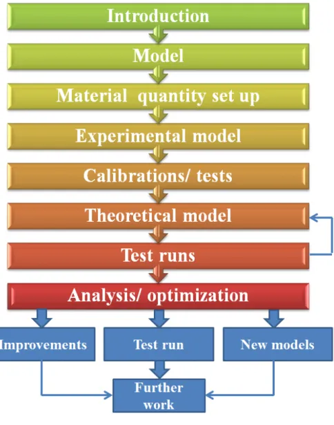
The optimization process resulted in some improvements and new design concepts. A new nozzle was designed and manufactured to investigate the new concepts through an opti-mization test run. The results have been analyzed and new nozzles for the further work was suggested. The working process in this thesis is described in figure 3.1

(24)

CHAPTER 3. METHOD M ¨ALARDALEN UNIVERSITY

(25)

4. Design and theory

This chapter includes description of a liquid cooling system in general, a theoretical model, design of the nozzle and technical description of the experimental cooling system.

4.1 Liquid cooling system in general

A liquid cooling system in general is based on a fan and a heat exchanger. The experimental model used in this thesis is similar to that of radiators in cars [9]. The principle of a heat exchanger is that hot liquid flows through a channel thermally connected to sheet metal plates in an airstream. During the passage, through the heat exchanger, the heat in the liquid is transferred to the air, which results in a lowered liquid temperature.

The liquid is based on water during normal conditions, but alcohol might be added at temperatures below 0◦C. Cooling capacity depends on several parameters, such as liquid flow through the heat exchanger, power supply and ambient temperature.

The direction of liquid flow through the heat exchanger is important to provide an efficient cooling. The liquid should flow against the airstream to obtain an optimum heat transfer. The principle of countercurrent heat exchanger is illustrated in figure 4.1 and is used in the test runs [10].

Figure 4.1: Principle of countercurrent heat exchanger

(26)

CHAPTER 4. DESIGN AND THEORY M ¨ALARDALEN UNIVERSITY

4.2 Theoretical model of the cooling system

This section includes a theoretical model of the experimental cooling system. The principle of heat transferring is generally described and then applied to the actual cooling system. Finally, the water spray is studied to obtain an equation that describes the impact of water spray.

4.2.1 Increase of temperature by the heating element

The amount of heating energy [11] required to increase the temperature ∆T† is in general described by the following equation:

∆Q = c· m· ∆T (4.1)

The mass of a followed element through the heating element is given by m0+ m. The energy

supply ∆Q is adopted by m while the energy in m0 is constant during stationary conditions.

The mass element of water is illustrated in figure4.2.

Figure 4.2: The mass element passes through the heating element

The mass flow through the heating element is given by:

φmass=

m ∆t

The mass flow φmass inserted into equation4.1gives:

∆Q = c· φmass· ∆t· ∆T

The volume flow through the heating element will be used in the test runs and is given by:

φ = φmass ρ =

m ρ · ∆t

The volume flow φ inserted into equation4.1 gives:

∆Q = c · φ · ρ · ∆t· ∆T

Power supply by the heating element is given by: ∆Q

∆t = c · φ · ρ · ∆T (4.2)

(27)

Temperature difference caused by the heating element (∆T = ∆THE) is described by:

∆THE=

∆Q ∆t ·

1

c · ρ · φ (4.3)

It is necessary to calculate the electrical power that applies to the heating element to understand how much heat the water is subjected to [12]. The electrical power is given by:

∆Q ∆t =

√ 3· U · I

A relationship between power supply ∆Q_∆t and increase of temperature ∆THE is obtained

by inserting the previous equation into equation4.3. This gives:

∆THE =

√

3· U · I · 1

c · ρ · φ (4.4)

However, the pump also contributes with some power P , which has to be considered. Equation4.4 gives:

∆THE = (

√

3· U · I + P ) · 1

c · ρ · φ (4.5)

4.2.2 Reduction of temperature by the heat exchanger

The ambient temperature in the test runs is 30, 40 and 50◦C. This will have an impact on the density and the specific heat capacity of the water, which has been compensated for [13]. Typical data for a test run is summarized in the following table:

Variable Value Unit Measured/appendix F

TIN− TOU T x ◦C x c 4177 J/kg · K appendix F ρ 988.1 kg/m3 _{appendix F} φ 0.219 · 10-3 m3/s measured U 400 V measured I 8.8 A measured P 30 J/s, W measured

Table 4.1: Typical data for a test run

Data inserted from table 4.1into equation4.5gives the increase of temperature caused by the electrical power supply:

∆THE = ( √ 3· U · I + P )· 1 c· ρ· φ = ( √ 3· 400· 8.8 + 30)· 1 4177 · 988.1· 0.219 · 10-3 = 6.78 ◦_C

The water temperature will increase by 6.78◦C with the data from above. It is important to notice that this is an average temperature increase over time and not an instantaneous value except for the case when the ambient temperature is 40◦C due to the change of specific heat and density. The average value will be studied in the test runs.

(28)

The system has to be in equilibrium, where TIN−TOU T is constant. The extracted power by

heat exchanger equals power supply by the heating element due to the equilibrium condition. This means that the increasing of temperature ∆THE equals the decreasing TIN − TOU T.

Equation 4.5 can be used to calculate TIN − TOU T caused by the heat exchanger and the

results are summarized in the following table:

P [W ] U [V ] I [A] TIN− TOU T [◦C]

30 400 4.3 3.33

30 400 8.8 6.78

Table 4.2: Result of the calculations in standard operation

4.2.3 Derivation of working temperature equation

The amount of energy required to vaporize water [14] with a total mass m is in general described by:

∆Q = Lv· m (4.6)

The mass of water spray that enters the cooling airstream and applies to the heat exchanger during time ∆t is given by m = ρw· V and the water flow through the nozzle is given by

ϕ = _∆tV . Water flow and density inserted into equation4.6 gives:

∆Q = Lv· ρw· V = Lv· ρw· ϕ· ∆t

∆Q

∆t = Lv· ρw· ϕ (4.7)

Equation 4.7 is valid in the ideal situation where 100% of the induced water vaporizes. This is not the case so an vaporization factor η has to be added to the equation. In this theoretical model, the ideal situation η = 1 is considered. The vaporization factor added to equation 4.7gives:

∆Q

∆t = Lv· ρw· ϕ · η (4.8) The water spray will maintain the same temperature as the ambient air and the heat exchanger will have a greater operating temperature. This means that the water in the spray will increase its temperature δT when it comes in contact with the heat exchanger. The estimated final temperature for all water induced is TIN. δT is then defined as the difference

between TIN and TA. This will generate an additional cooling effect due to heating of water

spray. δT inserted into equation 4.2and added to equation 4.8gives: ∆Q

∆t = Lv· ρw· ϕ· η + cw· ρw· ϕ· δT (4.9)

Before inducing water spray, ∆Q_∆t in equation 4.9 equals zero. The equilibrium condition gives:

∆Q

∆theat exchanger=

√

(29)

The different powers within the system are illustrated figure4.3.

Figure 4.3: Power supply and power extracted

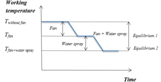
Equilibrium 1 in figure 4.4 corresponds to the working temperature (TOU T) in standard

operation of the system. The cooling capacity is affected when the water spray is induced. This results in a reduction of the working temperature and a new equilibrium will appear. The new equilibrium referred to as equilibrium 2.

Figure 4.4: Equilibrium 1 and equilibrium 2

Finally, to calculate the reduction of working temperature ∆T , equation 4.9inserted into equation 4.3gives:

∆T = Lv· ρw· ϕ· η + cw· ρw· ϕ· δT

c· ρ· φ (4.10)

(30)

4.2.4 ∆T by inducing water spray

The relationship between energy supply and water temperature in the ideal (boiling at 100◦C) [14] and the actual case is illustrated in figure 4.5. A large amount of energy is required to vaporize water, which is the process where liquid change its phase to gas. The actual vaporization of water spray will occur at a maximum temperature of TIN, instead of the ideal

which also is illustrated in the figure.

Figure 4.5: Relationship between energy required to vaporize and heating water

A comparison between heating and vaporization is made to illustrate how much energy it required in the vaporization process, as following:

1. Energy required heating 1 kg water 15◦C : ∆Q = c · m · ∆T = 4177 · 1 · 15 = 62.6 kJ 2. Energy required vaporizing 1 kg water: ∆Q = Lv· m = 2260 · 103· 1 = 2260 kJ

The vaporization of 1 kg water requires approximately 36 times more energy than heating it 15◦C. Typical data used in the test runs and in further calculations are summarized in the following table:

Variable Value Unit Measured/appendix F

∆Q ∆t x J/s, W x c 4177 J/kg · K appendix F cw 4175 J/kg · K appendix F ρ 988.1 kg/m3 appendix F ρw 992.2 kg/m3 appendix F δT 15 ◦C measured ϕ 0.02579 · 10-3 _m3_/s _measured Lv 2260 · 103 J/kg appendix F

Table 4.3: Data used in calculation with the water spray and in the test runs

Data from the table above inserted into equation4.9gives the required power to vaporize water and heat it 15◦C :

∆Q

∆t = Lv· ρw· ϕ· η + cw· ρw· ϕ· δT

= 2260· 103· 992.2· 0.02579· 10-3_{· 1 + 4175· 992.2· 0.02579 · 10}-3_{· 15}

= 59433 W

Where ∆Q_∆t equals extracted power by the water spray. The reduction of working temper-ature can be calculated by using equation4.10 and with data from table 4.3. This gives:

∆T = 2260· 10

3_{· 992.2· 0.02579· 10}-3_{· 1 + 4175· 992.2· 0.02579· 10}-3_{· 15}

4177· 988.1· 0.219· 10-3 = 65.8

(31)

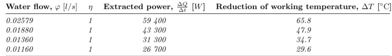
The results from the calculations with the other water flows ϕ are summarized in the following table:

Water flow, ϕ [l/s] η Extracted power, ∆Q_∆t [W ] Reduction of working temperature, ∆T [◦C]

0.02579 1 59 400 65.8

0.01880 1 43 300 47.9

0.01360 1 31 300 34.7

0.01160 1 26 700 29.6

Table 4.4: Results from water spray calculations with a 6 kW electrical power supply

The actual reduction of working temperature is measured in the test runs. This means that the actual η can be evaluated by modifying equation 4.10, which gives:

η = ∆T · c · ρ · φ − cw· ρw· ϕ · δT Lv· ρw· ϕ

, ϕ > 0 (4.11)

(32)

4.3 Design of the nozzle

The water nozzle was designed in collaboration with the supervisor at SAAB. This design was based on the cooling system specifications as following:

• The nozzle should easily be able to change between different configurations • An even distribution of water spray in the cooling airstream

A small dimension of the tubes was also sought in order to minimize drag in the air channel. The CAD model that is illustrated in figure4.6was manufactured and used in the test runs.

Figure 4.6: The manufactured water nozzle

The nozzle integrated into the duct, which is installed in front of the heat exchanger as illustrated in figure 4.7.

(33)

The hole dimension in the nozzle is an important parameter to produce an efficient spray. SAAB recommended that maximum diameter of the holes should be 0.5 mm. The final design resulted in smaller holes to produce smaller droplets. It is important to correlate the cross-section area of the horizontal tube to the cross-cross-section area of all the vertical tubes (8 tubes). Particularly important is to ensure that the area of all nozzle holes is smaller than the cross-section area of the horizontal tube. A situation where this condition is not met will lead to pressure drop and an uneven spray. This gives two conditions, as follows. The first condition is described by:

Ahorizontal tube > Avertical tubes

The nozzle dimensions inserted into the first condition gives:

Avertical tubes = 8 · πrv2

= 8 · π · 1.52 = 18π mm2 Ahorizontal tube> 18π

The internal diameter of the horizontal tube in the nozzle is 14 mm, so the first condition can be checked:

Ahorizontal tube = πrz2

Ahorizontal tube = π · 72 = 49π mm2

49π > 18π

Those eight vertical tubes have different number of holes, but it is fair enough to control the tube that has the most number of holes (20 holes), see appendix D. The second condition is described by:

Avertical tube> Aholes

The values inserted into the second condition gives:

Aholes= 20 · πr2h= 20 · π · 0.152 = 0.45π mm2

Avertical tube> 0.45π

The internal diameter of a vertical tube is 3 mm, so the second condition can be checked:

Avertical tube= πr2v = π · 1.52= 2.25π mm2

2.25π > 0.45π

Since there were many variables within the design of the nozzle, some of them were set as constants. For instance the distance between the holes was set to 20 mm and the distance between the vertical tubes was set to 43 mm. This was performed in CAD with different configurations to study its impact on the nozzle. The final configuration resulted in 132 holes divided into eight vertical tubes which are illustrated in figure 4.6. This was based on the two recently mentioned conditions as well as the specifications. For more detailed information about the configuration, see appendix D.

(34)

4.4 Experimental model of the cooling system

The experimental cooling system consists of following components:

• Pump: The purpose of the pump is to circulate cooling water. The water flow could be adjusted by the pump or the index valve. The pump has a power consumption which is added to overall heating of the water

• Heat exchanger: A water-to-air heat exchanger is used to extract heat energy from the water

• Heating element: A 3-phase heating element is used to supply heat energy to the water. It consists of two heaters that supply 3 kW each, together 6 kW

• Fan: The primary purpose of the fan is to circulate air through the heat exchanger. The second purpose is to break up water drops to produce water spray. The fan contributes to an increase of the surrounding temperature

• Index valve: The index valve is used in collaboration with the pump to control and regulate the water flow through the cooling system

• Nozzle: The purpose of the nozzle is to produce an evenly distributed water spray in the cooling airstream that enters the heat exchanger

A CAD model of the experimental cooling system and its components that used in the test runs are illustrated in figure 4.8. It also illustrates measure points, such as temperature probes.

(35)

5. Results

This chapter includes description of operating the cooling system, results from operating the system at different ambient temperatures with different power levels, test runs at standard operation as well as inducing water spray. It will also include evaluation of droplets size with different nozzle configurations.

5.1 Operating the cooling system

The electrical power supply can be calculated by measuring current and voltage that applies to the heating element. The electrical power is converted to heat energy by heaters within the heating element. This will increase the water temperature, which is illustrated as the red colored tube in figure 4.8. Water will be cooled when it passes through the heat exchanger, which is illustrated as the blue colored tubes in figure4.8. After the water has been cooled it enters a bucket that serves as an expansion vessel.

The cooling system was operated in a sauna with a volume of 12.8 m3 in order to simulate the system at different ambient temperatures. Heat emitted from the heat exchanger was used in order to achieve higher ambient temperature where needed in the test runs. The ambient temperature was regulated and maintained constant by closing and opening the door. Due to humidity and as a safety precaution the pump and heating element were placed outside the sauna during the test runs.

The water temperature was measured before and after it passed through the heat exchanger to study the cooling process. Water flow φ was controlled and regulated by the pump and the index valve. Parameters that have been kept constant in the test runs are shown in the following table:

Parameters Value

fan air flow 3605 m3_/h

water flow, φ 0.219 l/s

power (heating element), ∆Q_∆t 3 kW , 6 kW

amount of water in the bucket 16 l

pump power, P 30 W

index valve position 3.0

water flow, ϕ 0.0116, 0.0136, 0.0188, 0.02579 l/s

ambient temperature, TA 9, 30, 40, 50◦C

Table 5.1: Parameters and their values used in the test runs

The test runs have also been performed by inducing water spray. When the ambient temperature was stabilized at equilibrium 1, water spray was induced until the working tem-perature for the cooling system was stabilized at equilibrium 2.

(36)

CHAPTER 5. RESULTS M ¨ALARDALEN UNIVERSITY

5.2 Cooling system performance in standard operation

Several test runs have been performed to study the temperatures, such as the ambient tem-perature TA, inlet temperature TIN and outlet temperature TOU T. The focus was paid to the

test runs with 6 kW power supply, because this was of primary interest for SAAB.

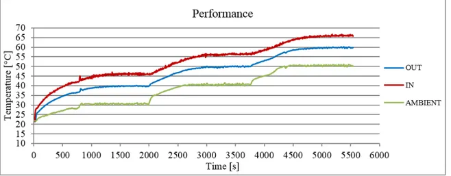
The relationship between TA, TIN and TOU T is illustrated in figure 5.1. This test run

operated for one and half hour with a 6 kW electrical power supply.

Figure 5.1: A test run of a 6 kW electrical power supply in standard operation

At the beginning, the system operated until the ambient temperature was stabilized at TA=30◦C. After a while, the blue and the red lines stabilized at approximately TOU T=40◦C

and TIN=45◦C. Every temperature level in the figure represents equilibrium 1 that was kept

for 20 minutes. The higher levels with stable temperatures TA=40◦C and TA=50◦C was later

achieved by closing the door and use the supplemental sauna heating element.

Main results from the test runs was a difference between TA and TOU T have maintained

(37)

5.3 Cooling system performance with water spray

The test run was performed with the same parameter specifications as in standard operation but with water spray induced. This test run had a water flow through the nozzle ϕ of 0.02579 l/s and its temperature in correspondence with the ambient temperature for each level. This test run operated for two and half hour in order to achieve a credible result on how the water spray affects the cooling capacity. The impact of water spray that is applied to the cooling airstream at a constant ambient temperature is illustrated in figure 5.2and 5.3.

Figure 5.2: Inducing water spray test runs with a 6 kW electrical power supply

Figure 5.3: Temperature difference caused by the heat exchanger and the water spray

With all temperatures stabilized at equilibrium 1, water spray was induced for approxi-mately 15 minutes at each of the three levels. The moment when the water spray was initiated and stopped is illustrated by purple arrows and orange arrows respectively in figure5.2.

(38)

5.4 Results from test runs

This section presents the reduction of working temperature between equilibrium 1 and equi-librium 2 at different ambient temperatures, water flows and electrical power supply.

5.4.1 ∆T with a 3 kW electrical power supply

Tables 5.2 - 5.4 summarizes the results of working temperature in the two different equilib-riums. These test runs were made with three different flows through the nozzle and three different ambient temperatures. For more detailed information about these test runs, see appendix A and appendix K.

Water flow ϕ=0.0116 l/s

TA [◦C] Tout(eq1) [◦C] Tout(eq2) [◦C] ∆T [◦C]

30 38.4 34.3 4.1

40 47.2 39.8 7.4

50 57.0 48.5 8.5

Table 5.2: TOU T and ∆T with a 3 kW electrical power supply and ϕ= 0.0116 l/s

30 37.5 32.5 5.0

40 46.0 39.7 6.3

50 55.2 45.2 10.0

30 36.0 33.8 2.2

40 45.1 37.8 7.3

50 54.9 41.7 13.2

(39)

The average value for the reduction of working temperature at a given ambient temperature is shown in the following table:

Ambient temperature, TA[◦C] Reduction of working temperature, ∆T [◦C]

30 3.8

40 7.0

50 10.6

Table 5.5: Average result of ∆T with a 3 kW electrical power supply at different TA

A comparison between test runs with and without water spray is illustrated in figure 5.4. The working temperature Tout is presented as a function of different ambient temperatures

TA = 30, 40 and 50◦C with a water flow ϕ= 0.0188 l/s at different equilibriums.

Figure 5.4: TOU T at eq1 and eq2 with a 3 kW electrical power supply

(40)

5.4.2 ∆T with a 6 kW electrical power supply

Tables 5.6 - 5.8 summarizes the results of working temperature in the two different equilib-riums. These test runs were made with three different flows through the nozzle and four different ambient temperatures. For more detailed information about these test runs, see appendix A and appendix K.

9 27.8 22.1 5.7

30 41.2 35.3 5.9

40 50.2 45.1 5.1

50 63.0 52.8 10.2

9 26.9 19.5 7.4

30 45.1 35.6 9.5

40 52.4 43.9 8.5

50 61.1 51.0 10.1

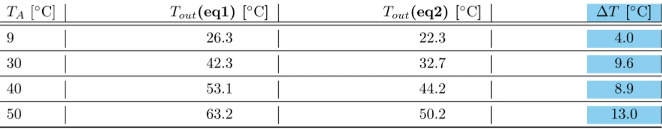
Water flow ϕ =0.02579 l/s

9 26.3 22.3 4.0

30 42.3 32.7 9.6

40 53.1 44.2 8.9

50 63.2 50.2 13.0

(41)

The average reduction of working temperature at a given ambient temperature is shown in the following table:

Ambient temperature, TA[◦C] Reduction of working temperature, ∆T [◦C]

9 5.7

30 8.3

40 7.5

50 11.1

Table 5.9: Average result of ∆T with a 6 kW at different TA

A comparison between test runs with and without the water spray is illustrated in figure5.5. The working temperature Tout is presented as a function of different ambient temperatures

TA = 9, 30, 40 and 50◦C with a water flow ϕ=0.0188 l/s at different equilibriums.

Figure 5.5: TOU T at eq1 and eq2 with a 6 kW electrical power supply

(42)

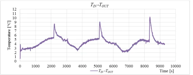
5.4.3 TIN-TOU T with a 3 kW electrical power supply

Tables 5.10 - 5.12 summarizes the results of TIN − TOU T in the two different equilibriums.

These test runs were made with three different flows through nozzle and three different ambi-ent temperatures. For more information about these test runs, see appendix A and appendix K. Water flow ϕ=0.0116 l/s TA [◦C] TIN− TOU T(eq1) [◦C] TIN− TOU T(eq2) [◦C] 30 2.9 2.5 40 2.1 2.5 50 2.2 2.7 Average 2.4 2.6

Table 5.10: TIN− TOU T with a 3 kW electrical power supply and ϕ=0.0116 l/s

Water flow ϕ=0.0136 l/s TA [◦C] TIN− TOU T(eq1) [◦C] TIN− TOU T(eq2) [◦C] 30 2.2 2.7 40 2.6 2.8 50 3.3 3.5 Average 2.7 3.0

Water flow ϕ=0.0188 l/s TA [◦C] TIN− TOU T(eq1) [◦C] TIN− TOU T(eq2) [◦C] 30 3.2 3.4 40 3.1 3.4 50 2.0 2.6 Average 2.8 3.1

(43)

5.4.4 TIN-TOU T with a 6 kW electrical power supply

Tables 5.13 - 5.15 summarizes the results of TIN − TOU T in the two different equilibriums.

Those test runs were made with three different flows of nozzle and four different ambient temperatures. For more information about those test runs, see appendix A and appendix K.

Water flow ϕ=0.0116 l/s TA [◦C] TIN− TOU T(eq1) [◦C] TIN− TOU T(eq2) [◦C] 9 4.2 4.6 30 3.4 4.2 40 4.9 3.9 50 4.6 4.3 Average 4.3 4.3

(44)

5.5 Evaluation of droplets size

This section is an evaluation of droplet diameter from different hole diameters on the nozzle. Figure 5.6 illustrates the water droplets exiting the hole that had a diameter of 0.1 mm. The picture was taken in a dark room with an illumination time of 1·10-6 s. The evaluation made with CAD to simplify the measurement of the droplets diameter. The droplets size was determined by measuring the vertical diameter. It is also important to mention that the tube has a diameter of 4.0 mm, which has been the reference in the measurements.

Figure 5.6: Droplets exiting the 0.1 mm hole

The same test run was performed with a 0.3 mm hole to study the impact of an increased hole diameter. Figure5.7illustrates the droplets exiting 0.3 mm hole.

Figure 5.7: Droplets exiting the 0.3 mm hole

Further measurements were also performed with hole sizes 0.2 and 0.4 mm. The results from all measurements are presented in the table below. For more information about these pictures and the selection of droplets, see appendix B.

Diameter 0.1 hole 0.2 hole 0.3 hole 0.4 hole

minimum [mm] 0.16 0.29 0.33 0.32

maximum [mm] 0.39 0.44 0.65 0.68

average (25 droplets) [mm] 0.30 0.37 0.44 0.46

ratio (droplet/hole) 3.0 1.84 1.48 1.15

(45)

6. Analysis and optimization

This chapter includes evaluation of different parameters, such as thermal resistance and va-porization factor, in order to obtain knowledge of the actual impact of the water spray. It also includes processing of the results and optimization of the entire cooling system.

6.1 Thermal resistance

Thermal resistance rtherm is generally used to estimate the temperature difference between

the heat emitting component and the ambient temperature. Thermal resistance [15] is defined by the following equation:

rtherm=

TIN− TA ∆Q

∆t

(6.1)

Where ∆Q_∆t is the actual measured power supply by heating element. Thermal resistance has been studied in order to explain the actual impact of water spray. Results from analyzing thermal resistance with different electrical power supply, water flows and ambient tempera-tures are illustrated in figure 6.1 and 6.2. The solid lines represents rtherm before inducing

water spray at equilibrium 1 and the dotted lines represents rtherm with water spray induced

at equilibrium 2.

Figure 6.1: Impact of water spray on the thermal resistance with a 3 kW electrical power supply

(46)

CHAPTER 6. ANALYSIS AND OPTIMIZATION M ¨ALARDALEN UNIVERSITY

Figure 6.2: Impact of water spray on the thermal resistance with a 6 kW electrical power supply

6.2 Processing of the results

The test runs defined as equilibrium 1 gave a TIN− TOU T considerably lower than expected.

The power supply equals power extracted at equilibrium. It is therefore possible to calculate the actual effect from TIN− TOU T using data from tables5.10- 5.15. Data from the first row

in table5.10inserted into equation4.2 gives: ∆Q

∆t = c · φ · ρ · (TIN− TOU T) = 4175 · 0.219 · 10

-3_{· 992.2 · 2.9 = 2631 W}

This means that actual power supply by the heating element was 2631 W (400 W lower than expected). It turned out that a small portion of air was enclosed in the heating element, which increased the thermal resistance between the heating element and the water.

The actual measured power has been considered in the earlier presented calculations and results. Results from calculations of the actual power supply are summarized in the two tables below. The first table shows data for the test runs with a 3 kW electrical power supply and the second table shows it for 6 kW electrical power supply.

TA [◦C] ∆Q_∆t(ϕ = 0.0116) [W ] ∆Q_∆t(ϕ = 0.0136) [W ] ∆Q_∆t(ϕ = 0.0188) [W ]

30 2631 1996 2903

40 1898 2350 2802

50 1980 2970 1800

Average 2170 2439 2502

(47)

CHAPTER 6. ANALYSIS AND OPTIMIZATION M ¨ALARDALEN UNIVERSITY TA [◦C] ∆Q_∆t(ϕ = 0.0116) [W ] ∆Q_∆t(ϕ = 0.0188) [W ] ∆Q_∆t(ϕ = 0.02579) [W ] 9 3800 3981 3438 30 3084 3992 4264 40 4429 4339 4791 50 4140 3790 4230 Average 3864 4023 4181

Table 6.2: Actual power supply by the heating element (6 kW)

The average of actual power supply can be calculated using data from table 6.1 and 6.2. The actual power supplied to the water was 2.4 kW with 3 kW electrical power supply to the heating element and a 6 kW electrical power supply resulted in 4.0 kW power supplied to the water.

6.3 Evaluation of vaporization factor, η

The ideal situation (η =1) was studied in the theoretical model, where all water vaporizes. This is not the case, so the actual vaporization factor for the different test runs can be calculated using data from tables 5.2- 5.8. Data from the first row in table5.2inserted into equation 4.11gives: η = ∆T · c · ρ · φ − cw· ρw· ϕ · δT Lv· ρw· ϕ = 4.1· 4175 · 992.2 · 0.219 · 10 -3_{− 4175· 995.7 · 0.0116 · 10}-3_{· 10} 2260 · 103· 992.2 · 0.0116 · 10-3 = 0.124

The vaporization factor in this case was 0.124. Results from calculations for η at different ambient temperatures and water flows ϕ are illustrated in figure6.3and6.4. For more detailed information, see appendix G.

Figure 6.3: η at different TA and ϕ with a 3 kW electrical power supply

(48)

Figure 6.4: η at different TA and ϕ with a 6 kW electrical power supply

6.4 Optimizing the nozzle and the cooling system

This section includes optimization of the entire cooling system to provide greater cooling capacity.

6.4.1 New design concept

As mentioned earlier, there are some constants involved in equation4.10. Vaporization factor η is the factor which has the largest impact on the cooling capacity. The first nozzle was not so efficient as expected, see figure6.3 and6.4. An explanation for this might be that the airstream had a bad access to the water beam as illustrated in figure 6.5. Therefore a new design concept was suggested where the spray angle has been changed from streamwise to perpendicular to airstream, see figure 6.6. The airstream will access the water beams easier and force it to break up in droplets more rapidly.

Figure 6.5: Water beam, streamwise configuration

(49)

6.4.2 Improving ∆T further

With the new design concept the vaporization process will be more efficient and will reduce the working temperature further. Another method to achieve greater cooling capacity is to increase the water flow ϕ. This will according to figure 6.3 and 6.4 reduce η due to the heating of droplets δT . However, the total cooling capacity will be greater due to the larger amount water supplied. This means that the system will be cooled by water rather than by the vaporization process. This was not sought in this thesis. In addition, increase of water consumption considered to be disadvantage.

Another method to improve ∆T further is to reduce the hole diameter, which will increase the area/volume ratio of the droplets. Droplet size can be estimated from a known hole diameter. Table 6.3 shows how the droplet dimensions are affected by changing the hole diameter. Small droplets will result in a larger wet surface that will be applied to the sheet metal plates on the heat exchanger.

Hole diameter [mm] Droplet diameter [mm] Area [mm2] Volume [mm3] Ratio A/V

0.1 0.30 0.283 0.0141 20.0

0.2 0.37 0.430 0.0265 16.2

0.3 0.44 0.608 0.0446 13.6

0.4 0.46 0.664 0.0509 13.0

Table 6.3: Droplets dimensions

6.4.3 Evaluation of the new design concepts

A test run to evaluate the new design concepts was performed. A new nozzle was designed and manufactured to have transverse holes with diameter of 0.1 mm. This nozzle satisfies the earlier mentioned area conditions. The test run has been made with the same parameter specifications as earlier, except for the actual power supply, now taken as 6 kW, and the water flow ϕ was changed to 0.00237 l/s. This flow was achieved by increasing the pressure in order to overcome the larger resistance due to the smaller holes. The results of the working temperature in the equilibriums and its reduction are summarized in the following table:

30 41.9 38.3 3.6

40 51.5 47.6 3.9

50 61.6 57.0 4.6

Table 6.4: Results of ∆T with the new design concepts

It is not fair to compare the reduction of working temperature with the earlier test runs since the water flow ϕ in this case is essentially (80%) lower. Therefore the vaporization factor and thermal resistance have been analyzed.

(50)

An increase in the vaporization factor with the new nozzle has been achieved, see figure6.7. That because the smaller droplets size that have a larger tendency to vaporize due to the 0.1 mm transverse hole configuration that made it easier for the airstream to access the water beams and break them up into smaller droplets.

Figure 6.7: η in the new design concepts, compared with the earlier test runs

As mentioned earlier in Processing of the results section, a portion of air in the heating element was the source of error that lowered the thermal contact between the heaters and the water. This error was solved before this optimization test run was performed. The power supply in this test run was in accordance with the expected value.

The thermal resistance in standard operation (eq1) is lower comparing with the earlier test runs. Figure 6.8 shows a reduction of thermal resistance when water spray is induced. The difference between the black lines in figure6.8is not so large due to the fact that smaller water flow gave a smaller reduction of the working temperature.

(51)

6.4.4 Positioning of the nozzle

An investigation of fan air velocity was made to find out if improvements in the positioning of the nozzle could be done. This was performed with a pitot tube that measured the local air velocity. By measuring the air velocity at different radius from the center of the fan, a profile of the velocity could be drawn. The positioning of the nozzle integrated with the profile is illustrated in figure 6.9.

Figure 6.9: Positioning of the nozzle integrated with the local air velocity

The variation of local air velocity with the radius is shown in the following table:

Radius, ri [mm] Local air velocity, vi [m/s] i

195 4.5 1 175 10.0 2 155 12.0 3 135 11.0 4 115 6.0 5 95 5.0 6 75 7.0 7 55 6.0 8 35 4.8 9 15 4.0 10

Table 6.5: Variation of local air velocity

The nozzles that was manufactured seemed to be ineffective in this context. The larger part of the holes were placed in low dynamic pressure areas while only few holes were placed in high dynamic pressure areas near the edge. This made the nozzles less effective and may be an explanation to the relatively large amount of water that came out from the drain hole in the heat exchanger.

(52)

The maximum air velocity was measured to be 12 m/s at a distance of 155 mm from the center of the fan and the minimum velocity was 4 m/s according to table6.5. According to the manufacturer, the fan should produce a maximum airflow of 3605 m3/h which corresponds to an average velocity of 8 m/s [16].

A calculation is performed to verify this value. Some important parameters needed in the calculation are illustrated in figure6.10.

Figure 6.10: Parameters used in calculation

The average air velocity is described by the following:

vaverage =

1 A

Z

v(r)dA

Where A is the duct cross section area. The parameters inserted into previous equation gives: = 1 π · R2 Z R 0 v(r) · r · 2πdr

Rewriting the integral as a summation of the local air velocities at different radius gives:

= 1 π · R2 n X i=1 v(ri) · ri· 2π∆r = 2∆r R2 n X i=1 viri

Data from table6.5 inserted into the equation gives:

= 2 · 20

2002 (4.5 · 195 + 10 · 175 + ...) = 8.22 m/s

The average air velocity from this investigation was 8.22 m/s which is close to the given value of 8 m/s by the manufacturer.

New nozzles were designed in consideration of the variation of air velocity and the new design concept with transverse holes. This resulted in two suggestions that differ from each other dimensionally.

(53)

The first suggestion is a circular nozzle configuration with a diameter of 310 mm that has transverse holes. This nozzle is placed along with radius 155 mm facing the maximum air velocity peak, which is illustrated in figure6.11a.

The second suggestion is a nozzle which has a diameter of 240 mm. This nozzle is placed between the two peaks, as illustrated in figure 6.11b. The size of the holes should be as small as possible due to the greater cooling capacity with smaller droplets. The benefit with the first suggestion is that it is possible to operate the system with a lower pressure to the nozzle, unlike the second suggestion where a higher pressure is needed to reach the peaks and to obtain higher water spray densities. The circular nozzle configurations will require better manufacturing equipment.

(a) Suggestion 1 (b) Suggestion 2

Figure 6.11: Circular nozzle configurations

6.4.5 Other improvements

It has been found from the test runs that airstream that passes through the heat exchanger is disturbed by the rear panel. The cooling system should also be able to operate under extreme conditions, so a protection is needed to prevent damage to the equipment. A suggestion to solve these problems is to replace the ordinary panel with an expanded metal mesh panel which is illustrated in figure6.12.

Figure 6.12: The expanded metal mesh panel

(54)

The new panel will give the airstream a more clearway. This will contribute to an even airstream distribution, which will also prevent damage to the sheet metal plates of the heat exchanger. The rear panel is illustrated in figure6.13.

Figure 6.13: A cross-sectional view of the heat exchanger

6.4.6 Optimizing water consumption

In the general test runs the water spray was induced constantly until the temperatures were stabilized. This resulted in a large water consumption. In order to optimize the water sumption, a test run was performed where duration for inducing the water spray was con-sidered. Figure 5.3 from section 5.3 showed that TIN − TOU T is reduced although the spray

was induced. This does not seem to be so effective. The water consumption for the system could be minimized by inducing the water spray until the maximum TIN − TOU T is reached.

It was found from the test runs that this appeared after approximately one minute (average 68 seconds), so the inducing could be stopped at this time.

Figure 6.14 illustrates a test run where inducing of water spray was stopped after one minute to study the time required for the system to return to its working temperature at eq1. The duration for peak value depends on the amount of water in the bucket and the water flow φ through the heat exchanger. All test runs were made with 16 l water in the bucket and a water flow of φ=0.219 l/s. If a mass element is followed through the system, it will take

16l

0.219l/s = 73 seconds to go one cycle in the system. This is the inertia of the cooling system,

which is also illustrated by the exponential decrease of the red line in figure6.15.

(55)

If a large TIN− TOU T over the heat exchanger is sought, a large amount of water in the

bucket should be used.

The same test run but with different parameters is illustrated in figure 6.15. The ambient temperature maintained 50◦C during the test run when a water flow ϕ of 0.02579 l/s was applied. The peak occurred after 70 seconds before an exponential decrease in TIN − TOU T

occurred. If the induce of water spray had been continued, the working temperature would have begun to stabilize.

Figure 6.15: A test run with inducing water spray

The water spray has an impact on the cooling capacity after the water spray was turned off. It required 15.5 minutes to return to the working temperature. This concept will minimize water consumption but still approximately have the same cooling capacity.

6.4.7 Simulation of water spray use in a real application

Figure6.16illustrates how the water spray can be used in future applications. The water spray is induced during one minute and it can be shown that water spray has to be induced four times during one hour to keep the working temperature below 60◦C. A general thermal limit for a typical component can be illustrated by the orange line in the figure 6.16. The water spray could in a real application be induced manually or automatically when the temperature limit for the component is reached. It is also possible to pulsate the water spray during a short time interval to minimize water consumption.

Figure 6.16: Simulation of the water spray in a real application

(56)

(57)

7. Discussion

It has been shown through the theoretical model that the vaporization process requires sig-nificant energy. Heating of water spray has a small impact on the cooling capacity and if only that heat is considered, with a given water flow ϕ of 0.02579 l/s, it will result in a reduction of the working temperature by 1.8◦C. From the results it has been shown that larger reduction of working temperature occur. This shows that the vaporization contribute to a greater cooling capacity.

The test runs were performed at different ambient temperatures to investigate the impact of the water spray. In reality, the water spray is hardly needed except at higher ambient temperatures. The cooling system can, as it is, maintain the working temperature 10◦C above the ambient temperature with a 6 kW power handling and 5-6◦C with a 3 kW.

When the ambient temperature is high and the restrictions of the component are limited, it is possible to reduce the working temperature 11◦C by inducing water spray. This is an average value at 50◦C and indicates that it is possible to operate the system in greater ambient temperatures. Since the water spray shows a significant impact even at low ambient temperatures, it would be possible to handle higher effects.

The vaporization factor increased with greater ambient temperatures and was reduced by larger water flows ϕ. An explanation for this could be that the amount of water that will be heated is greater. Elements that affect η are:

• Ambient temperature • Water flow

• Design of the nozzle

Another way of describing the increased cooling capacity is as the reduction of thermal resis-tance. As seen in figure6.1and 6.2, the thermal resistance has been reduced by a factor of 2. This occurs in conjunction with the reduction of working temperature. The heating element increases the water temperature TIN− TOU T, which is constant at equilibrium. This means,

by equation6.1† that TIN reduces by the reduction of working temperature, in order to have

TIN − TOU T constant.

The power supplied by the heating element was not completely transferred as expected. The processing of results section shows that the actual power supplied was 2.3 kW and 4.0 kW instead of 3 kW and 6 kW. A portion of air in the system reduced the thermal contact between the heaters and the water. This problem was averted in the optimization test runs.

†_r

therm= TIN∆Q−TA ∆t

(58)

CHAPTER 7. DISCUSSION M ¨ALARDALEN UNIVERSITY

Table5.16 shows a reduction of droplet size with a reduced hole diameter. The measure-ments were performed with 25 droplets, which resulted in an average ratio between droplet diameter and hole diameter of 1.9. The ratio of 0.1 mm hole was large compared to the Rayleigh theorem and an explanation might be due to the predrilling that was performed in the manufacturing process. The resulting dyne shape may affect the droplets exiting the hole. Due to this it is more credible to say that the average ratio is 1.5 with the 0.1 mm hole excluded.

The nozzle with 0.1 mm transverse hole configuration gave a smaller reduction of working temperature due to the smaller amount of water in the spray. The water flow was limited due to operating pressure and the smaller aperture size. However, from the analyse of vaporization factor it was concluded that the 0.1 mm nozzle was more efficient. The reduction of working temperature would have been larger if the same amount of water had been applied as in earlier test runs. This indicates that the smaller droplets have a larger tendency to vaporize, as mentioned in the hypothesis. There is a difference in A/V ratio between the nozzles configurations (0.3 mm and 0.1 mm holes). The larger ratio contributed to a greater cooling capacity.

The optimized nozzle provided a more efficient spray distribution under the optimization test run. The subsectionOptimizing water consumptionshows that it is not fair to only look at the peak value of TIN − TOU T when inducing the water spray. The peak occurs because

of the cooling system inertia. The peak for each test run is generally increased with the ambient temperature. The effect of water spray shows directly on TOU T and the parameters

was constant during all test runs, which means that the increased value of TIN− TOU T means

that water spray has a larger impact at greater temperatures.

7.1 The results related to existing researches

According toState of the art (SOTA)section, earlier studies have proved that the droplets are primarily affected by liquid properties, spray pressure and spray angle. When spray pressure was evaluated, results showed that greater pressures (flow) through the nozzle will result in a better cooling capacity (due to the amount of water applied). It has also been shown that spray angle increases the vaporization efficiency due to spray distribution. The results from this thesis verify earlier studies, and it has also been proven that water spray can be integrated into cooling systems to provide greater cooling performance.

Evaluation of water spray as a boost function for a cooling system

M¨

alardalen University

School of Innovation, Design and Engineering

V¨

aster˚

as, Sweden

Thesis for the Degree of Bachelor of Science in Engineering

-Aeronautical Engineering 15.0 credits

EVALUATION OF WATER SPRAY AS A

BOOST FUNCTION FOR A COOLING

SYSTEM

Mohammad AL-Jumaily

Robin Lindfors Lindell

Examiner: H˚

akan Forsberg

Supervisor: Jacob Brynolf

Company supervisor: Harald Pettersson

Preface

Abstract

Acknowledgment

Nomenclature

Definitions

Contents

List of Figures

List of Tables

1. Introduction

1.1

Purpose

1.2

Problem formulation

1.3

Hypothesis

1.4

Delimitation

2. Background

2.1

SAAB

2.2

Support and Services

2.3

Applications

2.4

State of the art (SOTA)

3. Method

4. Design and theory

4.1

Liquid cooling system in general

4.2

Theoretical model of the cooling system

4.3

Design of the nozzle

4.4

Experimental model of the cooling system

5. Results

5.1

Operating the cooling system

5.2

Cooling system performance in standard operation

5.3

Cooling system performance with water spray

5.4

Results from test runs

5.5

Evaluation of droplets size

6. Analysis and optimization

6.1

Thermal resistance

6.2

Processing of the results

6.3

Evaluation of vaporization factor, η

6.4

Optimizing the nozzle and the cooling system

7. Discussion

7.1

The results related to existing researches