Car longevity in Sweden : A revised estimate

F V//särtryck

744

1989

Car longevity in Sweden: A revised estimate

Bernard P.Feeney, National Institute for Physical Planning

and Construction Research, Dublin, Ireland

Peter Cardebring, Swedish Road and Traffic Research Institute,

Linkoping, Sweden

Reprint from Transportation Research, Part A, Vol 22, No 6,

pp 455 - 465

w Väg'OCh 7}Efi/(- Statens väg- och trafikinstitut (VTI) * 581 01 Linköping Institutet swedish Road and Trattic Research Institute * S$-581 01 Linköping Sweden

Printed in Great Britain. © 1988 Pergamon Press pic0191-2607/88 $3.00 + .00

CAR LONGEVITY IN SWEDEN: A REVISED ESTIMATE

BERNARD P. FEENEY

National Institute for Physical Planning and Construction Research, Dublin, Ireland and

PETER CARDEBRING

Swedish Road and Traffic Research Institute, Linkoping, Sweden (Received 7 February 1988; in revised form 9 August 1988)

Abstract-Previous studies have tended to exaggerate car longevity in Sweden. This has arisen because of the inclusion in the car fleet of vehicles that are no longer roadworthy. This report presents survival functions for cars for the period 1965-1984 based on estimates of the true car fleet. The mean life expectancy of cars is calculated at 14.7 years for 1984, as compared with 9.4 years in 1965. This is some 2 years below previous estimates. However, median car life in Sweden is still 1 year above that in the United States, for example.

INTRODUCTION

The longevity of the car fleet has important impli-cations for the size and structure of the car market, the measurement of depreciation charges to be as-signed to vehicles, and the rate at which changes in technology and legislative actions, aimed at new cars, pervade the total car fleet. This paper presents es-timates of the life expectancy of cars in Sweden for the period 1965-1984.

In common with similar studies, life expectancy is estimated by examining the age distribution of ve-hicles in the car register. A special problem arises in the Swedish context because of the twofold clas-sification of vehicles within the register: a vehicle may be registered either as 'i trafik' (in use) or 'av-stalld' (not in use). Cardebring and Jansson (1985) have shown that of the total of cars not in use only one-third become active again. It is, therefore, wrong to assume that a vehicle's time of 'death," that is the point in time when it is no longer available for use on the road system, coincides with its deletion from the car register. Thus, before any life expectancy estimates can be made, the age distribution of the 'true' car fleet must be estimated. Prior to this, how-ever, a review of previous life expectancy estimates and the methods employed is required.

A REVIEW OF PREVIOUS ESTIMATES AND METHODOLOGIES Swedish estimates

Previous estimates of car life expectancy in Swe-den have been made by AB Svensk Bilprovning (The Swedish Motor Vehicle Inspection Company) and published in a series of reports (see, for example, AB Svensk Bilprovning, 1972 and 1975). The meth-odology used was to first calculate age-specific

scrap-455

page rates g(x), by comparing the vehicle register at two successive end-years:

Ni ¢.1 -NiZl~q °

q'(x) = (2.1)

where q'(x) is the annual scrappage rate for x year old cars in year t, and N/_,_, represents the number of cars first registered in year t - x - 1 still in existence at the end of year t.

The proportion of cars surviving to age x(P'(x)) was then calculated as

P(x) = []; (1 - g'(x)). (2.2)

In this method, which is the one normally used in human life table estimation, survival proportions are based on age-specific scrappage rates derived from the most recent vintage of vehicle achieving that age. Thus, the life expectancy estimates do not refer to vehicles of any specific vintage. This may be called the variable vintage method. The alternative ap-proach is to measure the survival proportions of a cohort of vehicles first registered s years ago, by examining scrapping from that cohort over the in-tervening period-the fixed vintage method. Thus, if an s year survival function is to be estimated in year t, the survival proportion is calculated as

N3$*"

P"3*(x) = v (2.3)

where P''(x) is the proportion of the fleet first reg-istered in year t - s that survives to age x years, N$*' is the number of vehicles first registered in

year t - s surviving to year f - s + x, and is the total number first registered in year t - s. How-ever, this has the drawback that an adequate de-scription of the survival function may be obtained only after a large number of years has elapsed, and the survival function thus obtained may be a poor indicator of the longevity of the current car fleet. It should also be noted that while the variable vintage method produces estimates that are open to the in-fluence of economic conditions in the current year t, the fixed vintage method reflects economic con-ditions over the past s years. The survival functions calculated by AB Svensk Bilprovning were not given mathematical form, but were typified by the median life expectancy calculated by interpolation. The me-dian life expectancy of Swedish cars was found to increase from 9.4 years in 1965 to 16.2 years in 1982. The most substantial increase took place during the period 1971-1973, when an increase of 2.0 years was recorded. Part of the reason for this lies undoubtedly in the fact that prior to 1971, the calculations were based on cars in use, whereas from 1973 onwards cars not in use were also included.;

By 1982 there was serious doubt as to whether the inelusion of all cars not in use was justified and no further calculations were made.

International estimates

Given the importance of the subject, it is surpris-ing that there is relatively little international research published on car longevity. What' is available falls into two categories: the first deals with the estima-tion of mathematical survival or age-specific scrap-page rate functions, while the second deals with ex-amining the determinants of year to year changes in scrappage rates.

Thoresen and 'Stella (1977) for Australia, Ernvall (1983) for Finland, Bennett (1976) for Great Britain, and Cramer (1958) for both the United Kingdom and the United States all estimate mathematical sur-vival functions. Both Ernvall and Cramer use vari-able and fixed vintage methods to calculate survival functions, which are then expressed mathematically using the logistic function in the former and the Gompertz in the latter. Median life expectancies ranging from 10.4 years (1971) to 13.2 years (1982) are measured by Ernvall for Finland using the vari-able vintage method, and 13.5 years (1969) using the fixed vintage method. Cramer worked with consid-erably older data and calculated mean life expectan-cies of 8 to 9 years for the United Kingdom (1936-1938) using the variable vintage method and 10 to 11 years for the United States (1930-1942) using the fixed vintage method. Both Thoresen and Stella and Bennett had only one year's age distribution to work with, so P'(x) was calculated from a knowledge of the age distribution of the car fleet in year i and the

TAB Svensk Bilprovning do not provide an estimate for 1972.

total number of cars registered in each year prior to t:

1 Ni-,

P'(x) = m- (2.4)

where N;_, represents the number of cars first reg-istered in year t - x and still in existence in year t. This may be called the approximate variable vintage method. It suffers from the disadvantage that the results can be related neither to a fixed vintage of cars or to annual economic conditions.

Thoresen and Stella fitted a logistic function and Bennett a negative exponential function; a median life expectancy of 13.6 years for Australia (1971) and a mean life expectancy of just under 12 years for Britain (1974) were established. Greene and Chen (1981) estimate annual age-specific scrappage rates on United States data for the years 1966-1977 using formula (2.1). After fitting a scrappage rate logistic function, they estimate a survival function covering the entire period. Thus, although they use the vari-able vintage method, the results are averaged over an 11-year period. A mean life expectancy of just under 10 years is calculated. Other related studies are those of Parks (1977), Walker (1968), and Man-ski and Golden (1983), who are not directly con-cerned with the estimation of survival or scrappage rate functions but with establishing the determinants of scrapping behaviour.

Ignoring Cramer's estimates, which relate to a now distant time period, the calculated life expectancies range from 10 years in the United States to over 16 years in Sweden. However, given the very different measurement methodologies and data time periods, and the use of both mean and median life expectan-cies, too much should not be made of such differ-ences. In addition, as indicated above, the Swedish results are further complicated by the inclusion of currently inactive vehicles that will never become active again. The purpose of this study is to provide a more accurate estimate of Swedish car life ex-pectancy and, if possible, make a valid comparison with data from other countries.

DATA PROBLEMS Inaccuracies in car fleet statistics

A special feature of the Swedish registration sys-tem is that vehicles are not required to be continu-ously taxed and insured. This provision arose, in the first instance, in the early 1920s when it was rec-ognized that because of the relative severity of the Swedish winter, many cars were simply unusable for several months of the year. The inequity of taxation without possibility of use led the authorities to in-troduce a two-tier registration system, in which ve-hicles could be registered as 'in use' or 'not in use." For ease of reference, vehicles in these categories will be referred to as 'active' and 'passive'

respec-tively. Active cars (AC) must pay the Fordonskatt ease with which vehicles could be made passive and (annual vehicle tax) appropriate to their taxation> the relative difficulty of deregistering them.+ class and must be currently insured; passive cars (PC),

on the other hand, are entitled to tax and insurance refunds for the period of time for which they are passive. This dual system was reviewed in 1971 (SOU, 1971) and retained principally to allow commercial vehicle owners to continue to obtain tax refunds for vehicles in periodic use. The review body retained the system for private cars also, believing that their use of the passive status would. be low or confined to some special cases. While the original intention of the legislation was to allow vehicles to be win-tered, they can be rendered passive for other rea-sons, too: if, for example, vehicles are undergoing repair of a long-term nature, or if the vehicle owner is suffering from a lengthy illness, or going abroad for an extended period.

The use made of this flexibility in the registration system was not, until recently, substantial. In 1960, for example, only 52,300 cars, or 4% of the car fleet, were registered as passive. By 1970, the equivalent figures were 134,300 and 5.5% . The most substantial increase in the number of passive cars took place during the 19705: in 1977, the numbers rose by 123,300 to 337,900 and in 1979 by 60,500 to 450,900. By 1984, the tötal number passive stood at 631,000, or 17% of the car fleet.

These increases in the passive car fleet can be traced to a number of changes in the registration, tax, and insurance systems relating to vehicles. First, following computerization and centralisation of the vehicle register in 1972, the administrative charges for moving a vehicle from active to passive status, and vice versa, were abolished, and tax refunds were automatically forwarded rather than requiring a spe-cial written application on the motorist's part. Sec-ond, in 1979, insurance practices were changed with the result that car dealers were charged in relation to the number of days in which vehicles in their possession were in use and not on the basis of the total annual number of vehicles passing through their hands. Third, also in that year, the Fordonskatt lev-ied on cars was increased by almost 75%. As a result of these changes, the financial incentive to make a car passive was increased and the administrative dif-ficulty of doing so was reduced. The increasing num-ber of passive cars would not, in itself, constitute a problem for the estimation of car longevity provided such cars eventually returned to active status. How-ever, Cardebring and Jansson (1985) have assembled substantial evidence to show that this is not the case. By examining vehicle flows to and from the active register for the period 1976 to 1982, they estimated that of a total of 631,000 passive cars in 1984, 243 ,000 would eventually be brought back into active status; of the remainder, 100,000 would eventually be de-registered while another 300,000 were likely to main in the passive register indefinitely, unless re-moved by administrative f;at. The existence of this latter category of vehicles can be attributed to the

Thus, of the total passive, just over one-third re-turn to active use. The implication is that neither of the two alternative and readily available measures of the car fleet-the active fleet (AC) and the total-active plus passive-fleet (T) is a good indicator of the true car fleet that is available for use (TU). To obtain an estimate of the true car fleet, one must add the temporarily passive PCT to the active, i.e.

TU = AC + PCT. (3.1)

Cardebring and Jansson used this approach to re-construct a series to represent the true development of the car fleet over the period 1976-1984. This was subsequently used as an input to a car forecasting model for Sweden (Jansson, Cardebring, and Jun-ghard, 1986). This series showed that since 1976, the divergence between the active car fleet and the true car fleet had grown from 80,000 vehicles to 243,000 by 1984. These inaccuracies in the car fleet statistics indicate that neither the active nor the total fleet are suitable for the purposes of measuring car longevity. Previous estimates of median life expectancy have, most recently, been based on the total car fleet, and have, therefore, tended to overestimate car life ex-pectancy during the late 1970s and early 19805.

A methodology for estimating the level and structure of the passive car fleet

In order to obtain data suitable for the estimation of car longevity, it was necessary to describe a three-way classification (by model year, make, and size) not only for active cars (AC), but also for tempo-rarily passive ones (PCT). Cardebring and Jansson (1985) estimated the total number of passive cars by examining the size of flows to and from the active register, and by applying a set of factors to determine the vehicular mix of such flows. As analysis of these flows could not be extended to identify model year, make, and size characteristics, an alternative ap-proach was developed based on an examination of the car register at successive year-ends. In addition to comprehensive data relating to the characteristics of the car (weight, length, fuel used, number of doors, tyre dimensions, etc.) and more limited information relating to the owner (name, address, private or company), the computerised vehicle register also contains data on the registration status of the car (active or passive) and date at which the car became passive. Thus, it is possible to identify, for a partic-ular year-end, which cars are passive and when they entered passive status.

{In order to deregister a vehicle, the owner must prove that the vehicle no longer exists, usually by obtaining a certificate from an authorised scrapyard. This may involve costs of transporting the vehicle to the scrapyard.

+ An estimate of the number of cars in the P" category was made for one year, 1985. It was established that only 3,300 cars fell into this category.

End of Year End of Year

X X + 1

Active p

%

Active

]

[ Passive

mm +

[ Passive

|L - -P -~

- ---

Passive

]

&

$ ss

Nog 5 >- p i

N

|

.

>>

.

Deregistered ]» mr s l me

Deregistered ]

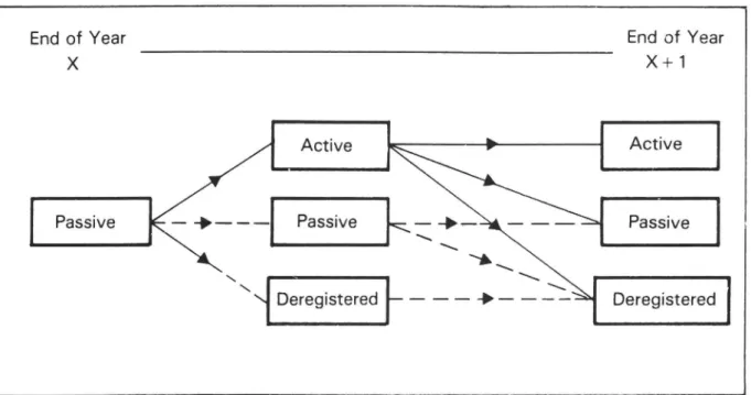
Fig. 1. Alternative registration patterns for passive cars.

In order to identify temporarily passive cars, it

was necessary to determine whether cars, which were

registered as passive at a particular year-end,

sub-sequently returned to active status. The obvious

ap-proach is to compare vehicle registers at successive

year-ends and identify those cars that were passive

at the first year-end but active at the subsequent one.

However, it is possible for cars to become active

during the course of the year, but to have changed

status again by the year-end. Figure 1 depicts the

principal alternative registration patterns for passive

vehicles over the space of one year. The continuous

lines represent the registration patterns that are of

interest for the detection of temporarily passive

ve-hicles. In addition to those passive cars that become

active during the year and remained so (PCT ")

oth-ers may have become active but returned to passive

status by the next year-end (PCT ''). Cars that are

habitually wintered would exhibit this behaviour.

Another possibility is that cars passive at one

year-end might become active during the year but would

be subsequently deregistered before the next

year-end (PCT""). It was decided at the outset of the

study that few cars would fall into this category, for

two reasons. First, it was known that the bulk of

passive cars are either in the course of being traded

or wintered. Both these categories of car are

essen-tially roadworthy and are unlikely to be scrapped

within a short period of returning to active use. Cars

that are passive and undergoing long-term repair are

similarly unlikely to be scrapped immediately after

return to active use.t

In order to identify PCT" and PCT" cars, the

car registration file was sorted and matched by

tAn estimate of the number of cars in the PCT'

cat-egory was made for one year, 1985. It was established that

only 3,300 cars fell into this category.

registration number for successive year-ends.

PCT" cars were isolated by identifying those that

were passive at the first year-end and active at the

second. PCT" cars were determined by isolating

those that were passive at both year-ends but had

been active between those year-ends. This was done

for each cell in the age, make, and size

cross-clas-sification. A more complete description of these

pro-cedures, including the treatment of cars that remain

passive for more than one year, is contained in

Fee-ney and Cardebring (1987).

Results

Table 1 shows that, in 1984, there were an

esti-mated 3,276,000 cars available for use in Sweden.

As the total car fleet comprising active plus passive

vehicles was 3,712,000 vehicles, this implies that

436,000 registered cars must be regarded as

per-manently passive or scrapped. The total of 3,276,000

cars available for use is made up of 3,081,000 active

and 195,000 temporarily passive vehicles. Since 1965,

the number of temporarily passive cars has increased

sixfold and the number of permanently passive or

scrapped sevenfold. The number of permanently

passive or scrapped vehicles in the register began to

grow quickly from about 1973, when the fees for

moving a vehicle from active to passive status were

abolished and the procedure was also simplified

ad-ministratively. While the number of temporarily

pas-sive also showed some growth in the early 1970s, the

largest increase took place in 1977, when the annual

vehicle tax was increased and administrative

ar-rangements relating to insurance were changed.

The estimated true car fleet rose from 1,823,000

in 1965 to 3,276,000 in 1984, a compound annual

growth rate of 3.1%. However, while the annual

increase in car numbers invariably exceeded 70,000

in the period to 1976, it failed to do so again until

Table 1. Analysis of the total car register and estimated true car fleet, 1965-1984, thousands Passive

Permanently Estimated

or true car

Year Active Temporarily unroadworthy Total registered fleet

1965 1,793 30 60 1,883 1,823 1966 1,889 33 57 1,979 1,922 1967 1,976 37 56 2,068 2,013 1968 2,071 38 64 2,173 2,110 1969 2,194 41 76 2,310 2,235 1970 2,288 43 91 2,422 2,331 1971 2,337 46 87 2,489 2,403 1972 2,443 48 1874 2,510 2,492 1973 2,503 76 67 2,646 2,579 1974 2,639 61 91 2,791 2,700 1975 2,760 61 121 2,942 2,821 1976 2,881 65 150 3,096 2,947 1977 2,857 130 208 3,195 2,988 1978 2,856 138 252 3,246 2,995 1979 2,868 170 281 3,319 3,039 1980 2,883 181 312 3,376 3,065 1981 2,893 188 335 3,416 3,082 1982 2,936 203 358 3,497 3,140 1983 3,007 200 386 3,592 3,206 1984 3,081 195 436 3,712 3,276

+A substantial number of vehicles were administratively deregistered in this year.

Total Car T ,,. ota Numbers (thousands)"7 3.200 2.700 2.200 -o oi oa o aa a a a nii a a a a o r e n '66 '68 '70 '72 '74 '76 '78 '80 '82 '84 Year Fig. 2. A comparison of the active, true, and total car fleets, 1965-1984.

460

1984. Thus, the compound annual growth in the pe-riod 1976-1984 was only 1.3% . Figure 2 depicts the trend in the active, true, and total car fleets since 1965. It can be seen that whereas the active fleet actually fell in 1977 and 1978, this apparent decline in car numbers disappears when temporarily passive cars are included. This supports Cardebring and Jansson's finding.

CAR LONGEVITY Alternative forms of survival functions

The previous section hås described how the age distribution of the true car fleet was derived for the years 1965-1984. Survival functions were then esti-mated using the variable vintage method. The age-specific scrappage rates g(x) were calculated by

3. ""

NM-s-qt(-x) so t-x ll 1 t-x l, t-x -1

(4.1)

where q'(x) is the annual scrappage rate for x year old cars in year t, and Ni_,_, represents the number of cars first registered in year t - x - 1 still in existence at the end of year t.

The proportion of cars surviving to age x was then estimated by

P'(x) = [T [1 - ax). (4.2)

Figures 3 and 4 depict scrappage and survival func-tions for the period 1965-1984, calculated in the above manner. A feature of the results is that scrappage rates tend to increase to a maximum and then either decline (pre-1980) or stabilise (post-1980). This lim-its the choice of mathematical form for the survival functions: the exponential functions exhibit a con-stant scrappage rate; the Gompertz, a continuously increasing one; while the Weibull permits a constant rate, increasing or decreasing scrappage rates de-pending on the parameter values chosen. The logistic function, on the other hand, has the advantage that it encompasses age-specific scrappage rates that rise to a maximum. For example, the simple two-param-eter logistic function:

1

m m (4.3) S(x) =

with the consequent scrappage rate function given by

10) =

dloiju)

D,

* see.

(4.4)

+We adopt the common convention of writing the

sur-vival proportion P(x) as S(x) when it is taking a specific

functional form. For a review of appropriate functional

forms, see Elandt-Johnson and Johnson (1980).

B. P. FEENEY and P. CaRDEBRING

Thus, the scrappage rate saturates at b,. An

addi-tional advantage of the two-parameter logistic

func-tion is that the median life expectancy-the age up

to which there is a 50% chance of survival-is simply

the quotient of the coefficients.

A variant on this functional form which has been

widely used in survival analysis is the

three-param-eter logistic function:

1

a + e-b0+blx

S(x) = (4.5) with the corresponding scrappage rate function:

b; Mx) = 1 + eto-hw

(4.6)

Estimates of car longevity

Both the above functional forms (4.3) and (4.5) were applied to the 1984 data, with the three-pa-rameter function exhibiting a slightly better fit. Table 2 presents the results. Thesurvival function was fit-ted using nonlinear estimation techniques, employ-ing the Gauss-Newton Method. A grid of starting values was posited (a = 0.9, 1.0; by, = 4, 5, 6; b, = 0.4, 0.5, 0.6) and the values a = 1, by = 6, and b, = 0.4 were selected. Thereafter, convergence was achieved in seven iterations. The corrected R was 0.9926 and all the coefficients were significant at the 1% level. The 1984 coefficient values were then used as starting values for the estimation of similar func-tions for the years 1965 to 1983.

The median life expectancy (MLE) is a convenient way of expressing longevity. Table 3 shows the cal-culated median life expectancy for the period 1965-1984. The estimates can be classified into three pe-riods: from 1965 to 1973, there was a steady increase in MLE, totalling 4 years in all (the year 1972, which provides an exception to this trend was, in all like-lihood, affectedby the changeover from local man-ual to central computerised records that occurred in that year); the second period covers the years 1974 to 1977, when a 1-year decline in MLE was recorded; in the third period, from 1978, life expectancy has once again grown steadily, registering a 2-year in-crease over the period. The median life expectancy now stands at 14.7 years (1984).

Perhaps the most interesting feature of Table 3is the decline in life expectancy that occurred in the post-oil-crisis period 1973-1976. This coincided with an increase in per capita private consumption of 10% over the same period, which represents an annual rate ofgrowth some 50% in excess of that for the previous five-year period. At the same time new car sales grew substantially to reach anall-time peakof 321,000 units in 1976. It may well be that the ad-ditional sales of new cars increased the supply of cars to the used market, thereby depressing used car prices and encouraging scrapping.

Scrappage Rate 0.3 0.25 0.2 - 0.15-T T T T T T. 7 T T T T T T T T T T T 1.7 3,7 5.7 7.7 9.7 11.7 13.7 15.7 17.7 19.7 Age

Fig. 3. Scrappage rate functions, 1965, 1970, 1975, 1980, and 1984.

Proportion Surviving 1.0 -0.9 - & 08 - .. +, .\ e 0.7 -

'..

no N

Table 2. Estimated logistic survival functions, 1965-1984 Year Parameter value ad bu 1984 1983 1982 1981 1980 1979 1978 1977 1976 1975 1974 1973 1972 1971 1970 1969 1968 1967 1966 1965 0.9367(0.0181) 0.9088([0.0263) 0.9350(0.0189) 0.9414(0.0220) 0.9510(0.0131) 0.9612(0.0125) 0.9798(0.0060) 0.9767(0.0073) 0.9779(0.0081) 0.9685(0.0116) 0.9539([0.0198) 0.9633(0.0133) 0.9873(0.0039) 0.9838(0.0072) 0.9826(0.0060) 0.9830(0.0076) 0.9840(0.0077) 0.9833(0.0077) 0.9909[0.0045) 0.9832(0.0082) 3.6832(0.2063) 3.2919(0.2513) 3.8557(0.2325) 3.9395(0.2793) 4.3332(0.1953) 4.4570(0.1947) 5.1736(0. 1188) 5.6469(0.1709) 5.767 (0.1957) 5.1748(0.2337) 4.6548(0.3340) 5.2087(0.2868) 5.7932(0.0996) 5.7859([0.1993) 5.3476(0. 1379) 5.9362(0.2145) 6.0317(0.2344) 5.6167(0.2267) 6.1063(0. 1806) 6.6126(0.2617) b, N R? 0.2468(0.0119) 30 0.9926 0.2197(0.0141) 30 0.9863 0.2694(0.0142) 30 0.9919 0.2878(0.0179) 30 0.9893 0.3180(0.0129) 30 0.9959 0.3349(0.0132) 30 0.9963 0.4048(0.0086) 30 0.9990 0.4479(0.0127) 30 0.9985 0.4537(0.0144) 30 0.9981 0.3999[0.0167) 30 0.9963 0.3539(0.0231) 29 0.9898 0.3824(0.0200) 17 0.9927 0.4872(0.0079) 17 0.9994 0.4606(0.0154) 16 0.9971 0.4531(0.0111) 16 0.9985 0.5092[0.0178) 15 0.9971 0.5332(0.0203) 14 0.9966 0.5061(0.0204) 13 0.9964 0.5918(0.0183) 11 0.9981 0.7100(0.0285) 10 0.9984 Note: Asymptotic standard errors are given in parentheses.

A comparison with other Swedish estimates

As mentioned in the literature review, previous estimates of car longevity in Sweden were under-taken by AB Svensk Bilprovning. These are depicted in Fig. 5, together with the estimates made in this study. For years up to 1971, the two sets of estimates are virtually identical. Thereafter, a substantial di-vergence is apparent that by 1982, the latest year for which AB Bilprovning make an estimate, amounts to 2.2 years-a median life expectancy of 16.2 years as compared with 14.0 years as calculated in this study. This difference arises because, for the latter years, the AB Bilprovning estimates are based on total cars, which, as has been shown, includes

sub-Table 3. The revised median life expectancy of cars in Sweden, 1965-1984

Year Median life expectancy

1965 9.4 1966 10.3 1967 11.1 1968 11.2 1969 11.5 1970 11.7 1971 12.5 1972 11.9 1973 13.5 1974 12.9 1975 12.6 1976 12.6 1977 12.5 1978 12.7 1979 13.2 1980 13.5 1981 13.5 1982 14.0 1983 14.7 1984 14.7

stantial numbers of permanently passive or unroad-worthy cars.

Because the two sources produce almost identical estimates for the pre-1971 period, the analysis of Swedish car MLEcan be extended by including AB Svensk Bilprovning estimates for the pre-1965 era (see Fig. 5). It is then apparent that the year 1965 represents a turning point in the MLE curve, and the general trend since then has been an upward one.

Mandatory annual vehicle inspection was intro-duced in Sweden in March 1965 for vehicles of five years old and greater. It is possible to view the changes in MLE as arising from this step. The decline in MLE during 1964 and 1965 could be attributed to the scrapping of vehicles in poor condition both in an-ticipation of inspection and arising from it. This would have weeded out deficient cars and resulted in the short-term reduction of scrapping rates of those re-maining. In subsequent years scrappage rates would continue to fall as cars would have higher accumu-lated maintenance expenditures than their pretest counterparts, and thus be in better condition. This process would have continued to effect MLE until the number of years, which have elapsed since test-ing began, exceeded the MLE. For example, in 1979, the MLE was just over 13 years where as 14 years of inspection had occurred. Thus, a car 13 years old in 1980 would have accumulated no more annual inspections than its 1979 counterpart, and ceteris par-ibus, a reduction in the scrappage rate for this age group could not be expected. MLE would not, there-fore, increase. This suggests that, whatever effect the introduction of annual vehicle inspection in-duced, it would have been exhausted by the end of the 19705. Examination of Fig. 6 reveals that MLE has continued to grow in the first half of the 19805,

Me di an Li feEx pe ct an cy Å 2 AB Bilprovning 16 =-This Study -a & 1 sa N 1 10 -T T TT T T T T wo T T T. T TA T T T T T > '64 '66 '68 '70 'Z2 '74 '76 '78 '80 '8g2 '84 Year

Fig. 5. Median life expectancy, 1965-1984: A comparison with estimates made by AB Bilprovning.

M e d i a nLi fe Ex pe ct an cy dp. Sweden 14 -USA 13 12 -11 j 10 - .\s~./, o . i T T * T 7 T T T T T T T (T > '71 "72 '75 '77 '79 '81 '83 Year

and this, together with the decrease in MLE in the early 1970s, suggests that factors other than annual vehicle testing have played an important role.

A comparison with car longevity in the United States

As mentioned before, a comparison of Swedish car life expectancies with those for other countries is difficult because of the use of different meth-odologies and data time periods. In order to provide a datum point for comparison with the Swedish re-sults, a study of car survival in the United States was undertaken that provided MLE estimates for the years 1971/72 to 1982/83. The data source was the Motor Vehicle Manufacturers' Association of the United States (1985), which in turn detives the data from R. L. Polk and Co.t The raw data consisted of the number of cars at July of each year classified by model year.

The method used to estimate survival proportions was the variable vintage method. It was then nec-essary to associate an exact age with each survival proportion. July is the observation date for each year, and it can be observed from car registration statistics that typically 65% of cars of a given model year are registered by that date. By linear interpo-lation, it is possible to estimate that the end of April is the approximate date at which 50% of cars of a given model year have been registered. This gives an age in year t for cars of model year t of 0.225 years.

Survival functions were then estimated for each year using the simple logistic function

1

Toman (4.7)

S(x) =

This was estimated by nonlinear least squares as be-fore. The results are exhibited in Table 4, together

with the calculated median life expectancy for each year.

A MLE for 1982/83 of 12.9 years was calculated. Exact year by year comparisons with the Swedish results are not possible, as the U.S. car fleet is re-corded in July of each year, and the Swedish in De-cember. However, Fig. 6 partially overcomes this by setting the U.S. estimates at the mid-year point. Two interesting features emerge. First; the U.S. experi-ence appears to mirror the Swedish but with a lag of approximtely 1.5 years: for example, the Swedish downturn of 1973 and upturn of 1978. Second, there is a tendency since 1978 for the gap between Swedish and U.S. values to converge, so that, whereas at the beginning of the period (1971/72) Swedish median car life expectancy was approximately 2 years above the U.S. value, by 1982/83 this had reduced to just over 1 year.

CONCLUSIONS

Previous studies have tended to exaggerate car longevity in Sweden. This has arisen because the method used, namely the comparison of the age dis-tribution of vehicles in the car register in two suc-cessive years, assumed that all such vehicles were available for use. However, vehicles may be regis-tered as active or passive and not all passive vehicles return to active use again. For example, this paper establishes that for the year 1984, out of a total of 3,712,000 cars in the register, 436,000 must be re-garded as permanently passive or scrapped. Thus, the true car fleet, available for use, was 3,276,000, of which 195,000 were temporarily passive vehicles. As previous estimates of car longevity were based on the total register, active plus passive, they have been seriously in error.

The number of passive cars in the register began to grow quickly from about 1973, when the

admin-Table 4. Estimated two-parameter logistic survival functions and median life expectancy of cars in the United States

Parameter values Estimated

median life Year by b; N R expectancy 1971/72 5.2119(0.0696) 0.5187(0.0068) 15 0.9995 10.1 1972/73 4.7703(0.0609) 0.4832(0.0060) 15 (0.9995 9.9 1973/74 5.2739(0.1146) 0.5061(0.0102) 15 0.9985 10.4 1974/75 5.3350(0.1703) 0.4660(0.0149) 15 (0.9961 11.2 1975/76 4.5424(0.1149) 0.4176(0.0105) 15 0.9973 10.9 1976/77 4.4338(0.0778) 0.4251(0.0074) 15 0.9987 10.4 1977/78 4.5003(0.1095) 0.4137(0.0100) 15 0.9974 10.9 1978/79 3.9228(0.1004) (0.3810(0.0096) 15 0.9970 10.3 1979/80 3.9525(0.1048) 0.3848(0.0101) 15 0.9968 10.3 1980/81 4,.5008(0.1621) 0.3785(0.0140) 15 0.9934 11.9 1981/82 4.4768(0.1444) 0.3689(0.0123) 15 0.9943 12.1 1982/83 4.9616(0.1978) 0.3860(0.0161) 15 0.9914 12.9

Note: Asymptotic standard errors are given in parentheses.

tThe authors would like to thank R. L. Polk and Co. (MVMA, 1985) for permission to use their data.

istrative fees for moving a vehicle from active to passive status were abolished and the procedure was also simplified administratively. Thus, relatively speaking, it became easier to make a car passive than to deregister it completely. This has resulted in the inclusion in the register of many unroadworthy ve-hicles. However, the active car fleet is not a suitable basis for estimating car longevity, either. For many decades, a substantial number of car owners have put their vehicles into passive status for the winter months. As the census of vehicles is undertaken at the end of December each year these wintered ve-hicles are excluded from the estimated active fleet, even though the majority of them are brought back into active use when weather conditions improve. Cars can be made passive for other reasons, too: if, for example, vehicles are undergoing long-term re-pair or are in the process of being sold. This report establishes that a major increase in the number of temporarily passive cars took place in 1977, follow-ing a substantial increase in vehicle tax levels and changes in the administrative arrangements relating to car dealers" insurance. Because of this growth in temporarily passive cars, the apparent decline in car numbers in 1977 and 1978, as measured by the active fleet, did not, in fact, take place. In the late 1970s and early 1980s the true car fleet has continued to grow, albeit at a much slower rate than in the pre-oil-crisis period.

Using the estimated age distribution of the true car fleet for the period 1965-1984, revised estimates of car longevity were made. The median life ex-pectancy of cars was estimated at 14.7 years (1984), which is some 2 years below previous estimates. However, this is still a full 5 years above the 1965 figure of 9.4 years. Median life expectancy grew strongly in the period to 1973, declined slightly in the post-oil-crisis period, and resumed its upward trend in 1978. The strong upward trend in the post-1965 period may be attributed in part to the intro-duction of mandatory annual vehicle inspection in that year. However, median life expectancy has con-tinued to rise during the early 1980s, when it would be expected that the impact of annual inspection would have fully worked through.

Few studies of median car life expectancy have been conducted for other countries. Those that are available make use of very different measurement methodologies and refer to different time periods and are, therefore, difficult to compare. This study has made estimates of car longevity in the United States and has shown that for 1982 median car life expectancy is 1 year below the Swedish level. A

decade ago, the difference was more substantial but there has been a gradual convergence over the pe-riod. Another interesting feature is that the U.S. estimates have tended to mirror the Swedish but with a lag of 1.5 years.

Acknowledgements-The authors wish to thank the Swed-ish Road and Traffic Research Institute for financing this research. The invaluable and efficient help received from Folke Carlsson of Statistiska Centralbyran is also acknowl-edged. The authors are indebted to their colleague Jan Owen Jansson for his many valuable comments. A longer version of this paper has appeared as a report of the Swed-ish Road and Traffic Research Institute.

REFERENCES

AB Svensk Bilprovning (1972) The Life Expectancy of Passenger Cars-Calculated in 1972. Vallingby, Sweden. AB Svensk Bilprovning (1975) The Life Expectancy of Passenger Cars in Sweden-Calculated in 1975. Val-lingby, Sweden.

Bennett T. H. (1976) The physical characteristics of the British motor vehicle fleet. Highway Eng. 23, (10), 24-29.

Cardebring P. and Jansson J. O. (1985) Avstallda bilar och Bilstatistiken. Meddelande 445. Statens Vag-och Trafik-institut, Linkoping, Sweden.

Cramer J. S. (1958) The depreciation and mortality of mo-tor cars. J.R. Stat. Soc. 121¥(1), 18-46.

Elandt-Johnson R. C. and Johnson N. L. (1980) Survival Models and Data Analysis. John Wiley and Sons, New York.

Ernvall T. (1983) The Service Life of Passenger Cars in Finland. Tie Ja Liikenne, The Finnish Road Association. Feeney B. P. and Cardebring P. (1987) The Longevity of Cars in Sweden. Rapport 321A, Swedish Road and Traffic Research Institute, Linkoping, Sweden.

Greene D. L. and Chen C. K. E. (1981) Scrappage and survival rates of passenger car and light trucks in the U.S. 1966-77. Transpn. Res. 15¥(5), 383-389. Jansson J. O., Cardebring P. and Junghard O. (1986)

Per-sonbils-innehavet i Sverige 1950-2010. Rapport 301, Sta-tens Vag-och Trafikinstitut, Linkoping, Sweden. Manski C. F. and Golden E. (1983) An econometric

anal-ysis of automobile scrappage. Transpn. Sci. 17(4), 365-375.

Motor Vehicle Manufacturers' Association of the United States (1985) Facts and Figures 1984. Detroit, Michigan. Parks R. W. (1977) Determinants of scrapping rates for post-war vintage automobiles. Econometrica 45(5), 1099-1115.

SOU (1971) Ett Nytt Bilregister Betankande av Bilregis-terutredningen. SOU, 1971:11. Kommunikations De-partementet, Stockholm, Sweden.

Thoresen T. and Stella P. (1977) Analysis of historical ve-hicle scrapping and survival patterns 1950-1976. Aus-tralian Transport Research Forum, Third Annual Meet-ing.

Walker F. V. (1968) Determinants of auto scrappage. Rev. Econ. Stats. 52, 503-506.