J
Ö N K Ö P I N GI
N T E R N A T I O N A LB
U S I N E S SS
C H O O LJÖNKÖPI NG UNIVER SITY
D o e s c h o i c e o f t r a n s i t i o n m o d e l
a f f e c t G D P p e r c a p i t a g r ow t h ?
Bachelor Thesis within Economics Authors: Emma Harrtell Hanna Larsson Tutors: Börje Johansson Tobias Dahlström Jönköping: January 2007
Kandidatuppsats inom Nationalekonomi
Titel: Påverkar val av omvandlingsmodel BNP tillväxten? Författare: Emma Harrtell
Hanna Larsson
Handledare: Professor Börje Johansson
Doktorand Tobias Dahlström
Datum: Januari 2007
Ämnesord: Ekonomisk tillväxt, omvandlingsekonomier,
marknadsekonomi, CEEC, chock terapi, gradualism
Sammanfattning
Efter upplösningen av Sovjetunionens starka maktkontroll över sina satellitstater den 9:e november 1989, kunde de Centrala och Östeuropeiska länderna (förkortning CEEC på engelska) påbörja sin övergång till marknadsekonomi. Sättet att närma sig en fri marknad är indelat i två olika tillvägagångssätt – chockterapi och gradualism. Den förstnämda metoden genomförs med fokus på snabbhet och en samverkande engångsförvandling av de ekonomiska sektorerna medan den sistnämnda beaktar en grad- och stegvis omvandling. Omvandlingsprocessen i sig består av flera variabler, exempelvis privatisering av statligt ägd egendom, makroekonomisk stabilitet samt liberalisering av priser och handel. Beroende på vilken metod som valdes genomfördes de ovan nämnda variablerna vid olika tidpunkter och med varierande hastighetsgrad. Åsikterna bland ekonomer rörande vilken metod som uppnått bäst resultat är omdebatterad. Följaktligen är syftet med denna uppsats att undersöka vilken av omvandlingsmetoderna som har uppnått högst BNP per capita tillväxt i de valda CEEC under perioden 1992-2003. Tio CEEC valdes ut för att få en rättvis delning mellan de två tillvägagångssätten, med tillhörande fem länder i varje grupp. Därtill valdes fem referensländer ut, för att i en grafisk analys kunna relatera utvecklingen i omvandlingsländer till redan etablerade marknadsekonomier. De erhållna resultaten visar att val av tillvägagångssätt inom omvandlingsprocessen inte har någon signifikant inverkan på BNP per capita utvecklingen. Ländernas grundförutsättningar samt i vilken ordning variablerna implementerades visar sig troligen ha större inverkan på BNP per capita tillväxten. Dessutom visar de empiriska resultaten klara indikationer på att det finns en skillnad mellan CEEC och referensländerna.
Bachelor Thesis in Economics
Title: Does choice of transition model affect GDP growth?
Authors: Emma Harrtell
Hanna Larsson
Tutor: Professor Börje Johansson
Ass.Tutor: PhD. Candidate Tobias Dahlström
Date: January 2007
Subject terms: Economic growth, transition economies, CEEC, market economy, shock therapy, gradualism.
Abstract
After the resolution of the Soviet Unions strict control over its satellite with beginning on the 9th of November 1989, the Central and Eastern European Countries (CEEC) began
their transition towards a market economy. How to approach the economic system of a free market has been divided into two major policies – shock therapy and gradualism. The first policy is implemented with speed and one-shock change within the economic sectors as a focus while the second constitutes of slow and gradual implementations. The transformation process in itself consists of several variables, for e.g. privatization of state-owned properties, macroeconomic stabilization and liberalization of prices and trade. Depending on what policy chosen, the variables were implemented at different times and with different speed. The views among economists regarding which of the two models that achieve the best result when transforming differs widely. Hence, the purpose of this thesis is to investigate which of the two models that have had the best effect upon the GDP per capita growth in the chosen CEEC. Ten CEEC were picked to have a fair representation for each policy, with five countries representing each policy group and the years measured were 1992-2003. In addition, for a graphical analysis to be performed and to distinct CEEC from already established market economies, five reference countries were included. The results obtained indicate that the policy choice has no impact on average GDP per capita growth. Instead we concure with earlier research that claim that preconditions and sequential order of the market reforms have a larger impact on GDP per capita growth. Additionally, empirical results indicated that there is a significant difference in the GDP growth over the last decade between our CEEC and the reference countries.
Table of Contents
Sammanfattning
...
i
Abstract
...
ii
1
Introduction
...
1
1.1 Method and Outline...1
1.2 Limitations... 2
1.3 Previous research... 2
2
Theoretical Background
...
3
2.1 Market Economy and its elements... 3
2.2 CEEC EU membership and market economy ... 5
3
Two ways of transformation
...
6
3.1 Shock therapy model... 7
3.2 Gradualist model ... 9
4
Empirical findings
...
11
4.1 Graphical analysis ...11 4.2 Regression Analysis...14 4.3 Regression Equations...15 4.4 Regression Results...164.4.1 Testing for BLUE...16
4.4.2 Hypothesis Testing...18
5
Analysis
...
22
6
Conclusion and suggestions for further studies ...24
References...25
Appendices
Appendix I Tables...28Graphs
1 Market Economy... 4
2 Command Economy... 4
3 Percentage GDP per capita growth...11
4 Annual percentage inflation rate ...12
5 Inward Foreign Direct Investment as a percentage of GDP...13
6 Openness Level ...13
7 Privatization Index ...14
8 Graphical test for autocorrelation in equation 4.1...31
9 Graphical test for autocorrelation in equation 4.2...31
Tables
1 White’s General Heteroscedasticity test...172 Correlation Matrix ...18
3 Regression Results for equation 4.1...19
4 Regression Results for equation 4.2... 20
5 Regression Results for equation 4.3...20
6 Descriptive Statitics of GDP between the groups ...21
7 The Jarque-Bera Statistics for regression 4.1...28
8 The Jarque-Bera Statistics for regression 4.2...28
9 The Jarque-Bera Statistics for regression 4.3...29
10 Durbin Watson Statistics...29
11 Total Regression results for equation 4.2...30
Figure
1 The Durbin Watson Decision Zones...29Introduction
1
Introduction
After the fall of the Berlin Wall in November 1989 a whole new era for the former Soviet Satellite States opened up - the transformation from a command economy to market economy. Some believed that the process would be easy and short. However, experience has showed that the transition process is complex, lengthy, difficult, and tackled different depending on which country you decide to study. However, the common denominator within the debate is the issue of policy choice when transitioning.
Hence, the big debate in the transition process has evolved around two different transition methods. Firstly shock therapy, also known as one-shock change or transformation model, which advocates a radical reform with a fast transformation to a market economy. Secondly the gradualist approach, a model promoting a rather cautious and slow evolvement of the economy and society. Nevertheless, even though one can identify two clearly different approaches within the transition process, it should be kept in mind that there are different scales within the two policies. Consequently, the shock therapy adonales use different speed levels and gradualists do not have one dominate school of reform (Åslund, 2002). Spokespersons from both sides advocate that their system is the best way to transform an economy. In addition there also exist economists who claim that the choice of reform speed has no impact upon the success or failure when transforming.
The purpose with this thesis is therefore to investigate which of the two transition methods, if any, that has achieved the best Gross Domestic Product (GDP) per capita growth in the Central and Eastern European Countries (CEEC).
The fact that the researchers’ opinions in this area are so different makes the topic very interesting to study. Furthermore, we regard this question to be highly relevant since out of the ten new member states of the European Union (EU), seven counts as transition economies. Additionally, more of the CEEC are on the path towards a future membership in the Union, and with that comes the importance of evolving into a market economy as this is one of the main requirements for becoming a member. Hence, to understand these countries’ role in the new and growing Europe, we find it crucial to study their background, as their recent history is characterized by revolutionary economic transformations.
1.1
Method and Outline
This thesis uses a confirmatory empirical analysis to conclude which of the views in this field of study that is the most accurate on the basis of the chosen years, countries and obtained statistical data.
Hence, the thesis will start by a theoretical framework to outline the historical background behind our purpose. Section 2 will explain the conditions needed to obtain a market economy. Further, section 3 will describe the two transition models; shock therapy and gradualism. Supported by the background theory, we will test our hypothesis in the empirical analysis. This will be done in sections 4 and 5 by using graphical and regression analysis. What will be examined is the influence that the choice of transition model has upon the GDP per capita growth of the transition economy. Finally, section 6 will conclude the thesis and give recommendations for future studies.
Introduction
1.2
Limitations
We have limited ourselves to the Central and Eastern European Countries. The chosen shock therapy countries and their starting year of transition are: Poland (1990), Czechoslovakia (1991) that in 1993 peacefully split into the two countries Czech Republic, and Slovak Republic, Bulgaria (1991) and Albania (1992). (Marangos, 2002) The gradualist countries are represented by; Hungary that initiated some reforms already from 1968 onwards (Hare & Révész, 1991), but primarily from 1989, Romania (1990), and the three Baltic States; Estonia, Latvia and Lithuania (1990). (Beyer, 2001)
The first reason for picking the above mentioned countries is that they are all situated close to a region that for a long time has had a working market economy. Moreover, when the CEEC joined, or potentially is joining, EU a market economy is one of the basic requirements. Furthermore, these CEEC also have the same background; that is being satellite states to the Soviet Union, and they started their transition process more or less at the same time in the early 1990s; the only exception being Hungary, that embarked on their transition as early as 1968. All of the now mentioned features make a comparison easier and more reliable than if we would have involved transition economies from other continents.
Finally, to make it easier to draw conclusions about the GDP per capita development of the chosen transition countries we will include five reference countries from Western Europe; Austria, the Netherlands, Finland, Greece and Portugal. The reasons for choosing these countries as reference countries are that they are already established members of the European Union in addition to that they are fairly equal in size to the chosen CEEC. However, these countries will only be mentioned if there is a significant finding in the data brought about by these states.
1.3
Previous research
This topic has been discussed by many researchers. One of the well-regarded researchers in this area is the pro-shock therapy economist Jeffrey Sachs (1997a & b) from Columbia University, whom also helped some of the CEEC to outline their transition strategies. As a counter-pool Oliver Blanchard from Cambridge University can be mentioned, as he strongly advocates the gradualist approach of transition. Nevertheless, there are also researchers who claim that choice of transition model has no effect upon the GDP development, and that there are other factors that influence GDP. The most interesting scholar is Jürgen Beyer (2001) from the Max Planck Institute for the study of society in Cologne but also John Marangos (2002 & 2005) from Colorado State University can be mentioned. Accordingly, extensive previous empirical and theoretical research has been done within this field. Among the empirical researchers is Andreas Johnson (2004) from Jönköping International Business School, who examined the large differences between the individual transition countries when it comes to attracting Foreign Direct Investment (FDI). He argues that the difference lies in what privatization method is used and that the performance of that method will affect FDI inflows.
Theoretical Background
2.
Theoretical Background
The transformation of socialist countries into democracies implies two fundamental forms of structural change because of the close relationship between economics and politics in socialist countries; first a political change from a communistic to a democratic regime and secondly an economic change from a command economy to a market economy. The later issue being the focus of the thesis. However, the question then is what constitutes a market economy. The elements will therefore be untangled and defined in this section.
2.1
Market Economy and its elements
The origin of the market economy goes back along time in history but basically it holds the same characteristics today as when one of its founding fathers, Adam Smith wrote his world renowned book “The Wealth of Nations” in 1776. This was when the phrase “the invisible hand” first was coined (Smith, 1910), implying that there is no governmental intervention or other coercion. Hence, it is a place where buyers and sellers meet and conduct trade, according to rules that are upheld by regulations, laws and self-organised behaviour. Additionally, it is also a natural place for transactions, transfer of property rights, and establishment of contracts. (Hacker, Johansson & Karlsson, 2004). This requires educated players with a fundamental understanding of the market and its features, knowledge often missing in transition countries. Building this is a time-consuming process and failure within this area can cause high levels of corruption. Hence, it is important to have stable and regulated institutions to counteract the possible corruption incentives (Marangos, 2005).
Even though institutions transform slowly, they have a strong influence upon economic performance and stabilization in a country. This stage can also be referred back to as the Achilles heel of the transition economies, as institutional building is the basis for a market economy (Marangos, 2005). The importance of these institutions becomes clear when one refers to how the state income has to be changed when moving from a command economy towards a market economy. In the command economy the state income mainly comes from the state owned enterprises (Åslund, 2002). When privatizing the enterprises the government loses the source of income that had been extracted from the profits of the state old businesses. Consequently, resources have to be searched for elsewhere, e.g. through tax collecting institutions.
Morover, a market economy is an economic system in which the production and distribution of goods and services takes place through the mechanism of free markets. This is guided by a free price system rather than by the state which is the case in a command economy (Isachsen, Hamilton & Gylfason, 1994). A functioning market economy or system needs to be able to adjust for competition and pressure from the market that comes with the supply and demand factor as a price decider (Hacker. et al, 2004) as can be seen from graph 1 on the next page.
Theoretical Background
Graph 1 – Market economy Graph 2 – Command Economy
Supply and demand under market economy Supply and demand under a command economy
In comparison, graph 2 highlight the fundamental difference between the two systems, where it can be seen that the command economy establishes the total production for x-period. The pre-determined production quantity S(q) that is determined by the state is fixed regardless of the demand, hence creating market distortions (Isachsen et al, 1994).
When moving away from a state owned system, where economic incentives are small it will most likely boost the willingness from owners of properties to perform better than before. (Estrin, 1998). As the market economy is mainly built by private investments the issue of risk and risk aversion arises when investing. The incentives for entrepreneurs to invest lies in the fact that they can profit from the investment, however with investments also comes the risk of losing. Moreover, when an enterprise is not profitable, the ability to close it down is a fact. As a result, free entry and exit becomes the pillars of this economic system (Cincera & Galgau, 2005). This is a non-existing phenomenon in a command economy. Consequently, privatization is necessary in the market economy for three reasons; (1) to free the public resources that had been used to subsidized inefficiency in the state-owned-enterprises. (2) to increase the size of the small private sector. (3) to promote both foreign and domestic private investment (Rondinelli, 1994). Thus, privatization attracts foreign direct investment (FDI). FDI in turn stimulates economic growth and capital accumulation. (Isachsen et al, 1994)
Another characteristic for the market economy is the ability to trade freely. Free trade enables the countries to define their comparative advantage and in a proper manner use it to derive profits from trade in the world market. The continuous movement towards free trade is essential for a successful transition to a market economy. Hence, promotion of growth in exports, limit the rise in imports and improve the trade balance in addition to the balance of payments (Marangos, 2005). The step to be able to interact in the world market has become known as liberalization, or openness as it is referred to in this thesis (Åslund, 2002). The process can be divided into two parts – price liberalization and trade liberalization, the latter including currency convertibility, the elimination of export controls and substitution of low to moderate import duties for import quotas and high import tariffs (Heybey & Murrell, 1998).
A functioning market economy also rests on the fact that the country has a somewhat maocroeconomic stability, hence resisting inflationary pressure. High inflation is, according to Jeffrey Sachs (1997a), almost always a result of fiscal imbalances and low confidence in the macroeconomic management. If a country experience high inflation it will be seen as instable and this affects trade and GDP negatively. Fiscal imbalances and low confidence in
Theoretical Background
macroeconomic management are often present in a command economy and become noticeable when trying to move into a market economy. (Sachs, 1997b)
2.2 CEEC EU membership and market economy
Due to the fact that a majority of the chosen CEEC now have joined the EU a list of demands for the accession has been put upon them. Firstly, the countries have to obtain stable institutions that secure democracy and uphold a functioning legal system. Secondly, all features of a functioning market economy must be established to enable the countries to compete with the other market forces within the Union. Lastly, the countries must have the ability to reinforce all the obligations that comes with a membership, such as joining the Economic and Monetary Union (EMU). To live up to the implementation of the common currency the inflation rate must be kept at bound of an average 2 percent. Higher inflation rates have been a constant problem for all the CEEC up until recently, and still some of the countries have not lived up to this goal. Although, the EU goal of an annual GDP growth of 4.5 percent has been reached for almost all of the CEEC, as opposed to the reference countries that have had troubles achieving this goal. (El-Agraa, 2004)
Two ways of transformation
3
Two ways of transformation
The main reason in favour of transition is the urge to put the CEEC in question on the course to a sustainable economic growth. It is believed that the shift of property rights from state to private owners and the change of allocation mechanism from the state to the free market will boost saving rates and capital formation, on top of obtaining allocative efficiency. (Kolodko, 1998)
When privatizing an economy there are many different paths and the decisions are very complex. The point lies in the decision if the country should to go through the process with speed and as a one-point transformation for all economic sectors, which the shock therapy spokespersons advocate. While the other option is letting transition take time and allow each step to become deeply implemented and mature into the economy, gradualism. Nevertheless, within all the command economies there are different steps that researchers claim affect the GDP growth in its own way, hence the independent variables; privatization, level of openness (Beyer, 2001), FDI (Johnson, 2005) and macroeconomic stabilization in the form of for e.g. inflation (Sachs, 1997a). From the author Jürgen Beyer’s (2001) empirical study you can find arguments in favour of that these different ingredients have varying weight and importance between the two systems.
The transition countries all came into the phase of transition with very different economic conditions. Also, along the transformation process the conditions varied among the countries. According to Beyer (2001) this fact will influence the result of their transition. As an alternative he claims that the preconditions and individual size of the economy are of more importance when estimating the success of the countries transformation. Jürgen Beyer (ibid) argues further that the sequence in which the country implements the different variables required to transform into a market economy is of more essence than whether the focus is laid on the one-shock change or the gradualist model.
A majority of the CEEC entered the transformation process with high inflation levels or under the threat obtaining it. Some researchers claim that it is the number one threat for transition economies. (Marangos, 2005) Although, for most of the chosen CEEC evidence show that inflation levels was fast brought under control after stabilization programs had been issued. (Fisher & Sahay, 2001) Regardless of transition model, the CEEC had the option of either fixing the exchange rate or allowing it to float. Countries from the two models are found in both of the two exchange rate regimes.
Within the privatization process there is the question of whom to privatize towards? Thus, different ways can be distinguished. Firstly, one can decide to privatize to the following persons; existing managers and workers, the general population, the previous owners, so called restitution and foreign and domestic private firms. Following the first choice, there is a two-fold alternative between either selling the properties or giving them away for free. (Estrin, 1998) Johnson, (2005) writes that this choice might have a substantial impact upon the level of success in the privatization advancement. Privatization in itself is a very important tool to improve economic efficiency (Welfens & Jasinski, 1994). The privatization process meant a movement from inefficient production and obsolete products regardless of what policy chosen. (Hacker. et al, 2004) A necessity in the transition towards a market economy.
Two ways of transformation
Furthermore, the privatization helps create opportunities for FDI to be attracted, as oppose to under a state-owned business economy. Some researchers even argue that choice of privatization method, and then most importantly the choice of whom to distribute the shares to during the privatization, have a significant effect upon the total level of FDI flows to the country. (Johnson, 2005) During the command economy era the economic beliefs was that of self reliance and total indecency from foreign investments. This changed as the transition process emerged (Johnson, 2004). The transition economies found themselves with a redundant capital stock that they had an opportunity to change by attracting FDI (ibid). However, there are some conditions crucial for the existence of FDI in the transition countries; (1) a stable market economy with secure property rights that protects the investors, (2) price liberalization was required since the foreign companies needed to be able to sell at their own prices and (3) openness in the form of increased trade levels. However, too much FDI is not the best option either, due to the loss of domestic ownership and by that the ability to generate export opportunities. (Bruzek, 2005)
Lastly, the continuous movement toward free trade is important for all the transformation countries, to enable them to improve their trade balances and balance of payments. Trade openness has been closely related to the privatization process due to the fact that the new private owners need export opportunities (Marangos, 2005). After November 9th, 1989
almost all the CEEC were able to shift their exports to Western Europe instead of just trading within their region. The planned economies of Eastern Europe had their own trade agreements called CMAE (Council for Mutual Economic Assistance) up until 1991. However, the economic benefits of this organization have been highly questioned. (El-Agraa, 2004) After the fall of CMAE the movement from centrally planned economies into transition economies emerged (Hacker. et al, 2004).
Before going in more deeply on what constitute shock therapy and gradualism it is important to get an understanding for when the transition is finalized. In accordance to Gelb (1999) this occurs once the transition economies have the same economic and policy problems as already established market economies. Hence, keeping this in mind is important for the understanding of how much a transition economy has to transform and sacrifice before reaching the same level as the prevailing market economies, such as the old EU members.
3.1
Shock therapy model
The name shock therapy, or one-shock change model as it is sometimes called, originates from Poland and their privatization path that was initiated on January 1st 1990. The model is of neoclassical thoughts and promotes that the market economy initiation steps should be taken fairly quick. Supporters of shock therapy argue that it would ensure a positive growth and full employment with a low inflation if the implementation of the necessary reforms were introduced somewhat simultaneous. There was no need to let each step mature into the economy since each part was equally important and together they were the bulks of the entire transformation. (Bruzek, 2005)
The steps that were taken and seen as necessary was immediate price liberalization and minimum state intervention through privatization. The privatization method, in the one-shot change model was undertaken quickly. A reason for this was that corruption constituted a major problem in many enterprises. The shock therapy countries argued that a slow privatization would rather trig the corruption incentives. (Åslund, 2002) These steps
Two ways of transformation
should be implemented without political interference and totally independent of the political part of the transformation process, moving towards democracy. Many of the one-shot change countries believed that when macroeconomic stabilization was reached everything else would fall into place for e.g. industrial policy, environmental policy, etc. (Nove, 1995).
The steps that the privatization process had to undergo was; restitution, small-scale privatization and large-scale privatization (Nemcova, 1998). Small-scale privatization often took place in form of auctions or domestic sales and was implemented without any major problems. Large-scale privatization was usually performed using privatization vouchers or coupons that were either distributed or sold. In what manner this was carried out varies between shock therapy countries. (Åslund, 2002) Also the issue of how many of the enterprises that were to be put up for privatization became an issue where the countries differed vastly. Nevertheless, the common feature was the fast pace of this entire process and the fact that future revenue would be obtained from the formerly state-owned enterprises that now was privately owned. (Marangos, 2005) However, the high speed level also caused some problems. The regulating institutions and legal systems did not have time to evolve during the short time span between the initiation of the entire transformation and the starting point of the privatization process. (Fisher & Sahay, 2001)
Disregarding the problem mentioned above, the shock therapy model saw privatization as a method to get the people in favour of the program. It was believed that if the program became popular among the inhabitants, the political support would help the implementation of the other stages within the transformation. (Marangos, 2002) However, in their request for a rapid transition they did not quite manage to get the people involved. Many countries initially strived for some enterprises to stay under domestic ownership, hence many times the first auction (performed with vouchers) were closed for foreigners. Since the public did not fully have time to adjust to the privatization process and thus comprehend the fact that they could buy shares in the enterprises, this failed. A second round was initiated and this time it was opened for foreigners, due to the need of monetary inflows. For foreign companies this was a bargain since companies were sold relatively cheap in addition to the existence of low labour cost in these countries. (Sachs, 1997b) This resulted in a high concentration of FDI in many shock therapy countries, Czech Republic being the most prominent example. (Bruzek, 2005)
The success of FDI in shock therapy countries can thus mainly be explained by the high levels of complete business sell-outs during the privatization waves (Johnson, 2005). However, there is also one down-side to the presence of FDI. When having high comcentration levels of FDI the domestic ownership might become so weak that the country is fully reliant on foreign income, in addition to foreign companies to uphold the labour market. This is quite common for shock therapy countries. (Bruzek, 2005)
The establishment of an independent Central Bank, international trade and a convertible currency was implemented as features of the countries’ liberalization process (Marangos, 2002). This gave the shock therapy countries the opportunity to restructure their trade model, letting exports be dominating (Åslund, 2002). They were then able to generate income and using their comparative advantage in a better way then they had been capable of during the command era. Examples of countries trying to improve their openness by a rapid liberalization was Czechoslovakia, (after 1993 the Czech and Slovak Republics) and Poland, whom in the very beginning of the transition process devaluated their currencies
Two ways of transformation
and by that improved their gross trade flow. Liberalization, openness and a devaluation of the currency aided these countries in their trade. (Sachs, 1997b)
Among the shock therapy spokesmen, inflation was thought to be one of the biggest problems that these countries were facing economically, due to the negative impact it had on growth. It was argued that massive inflation was a result of irresponsible governments during the command economy since these governments increased the money supply too excessively. (Marangos, 2002) According to Jeffrey Sachs (1997a) many of the transition countries benefited from having a temporary pegged exchange rate to control inflation. Principally because it is a clear signal from the government which may help stop a flight of currency. Thus it gives the states a chance to restore the domestic money supply (ibid). Most of the shock therapy countries eventually used their interest rate and their exchange rate to control inflation. Consequently they moved from a very loose monetary policy to a much stricter one, implemented through an independent Central Bank. (Åslund. 2002) The countries that fixed their exchange rate during the transition process were Czech Republic, Poland and Slovak Republic. While countries such as Albania and Bulgaria worked with a floating exchange rate. (Fischer & Sahay, 2001) Additionally, devaluation was another measure to fight the high inflation levels (Sachs, 1997a).
3.2
Gradualist model
On the opposite side of the one-shock change model is the gradualist approach, nonetheless also a neoclassical founded model. The main methods of this type of transformation are gradual and partial reforms aiming at elimination or reduction of the transitions negative impact on economic growth. Nevertheless, the final goal is identical with that of shock therapy – reaching a well-functioning market economy with a sustainable economic growth. (Bruzek, 2005) Although, as oppose to the shock therapy the order in which to implement the free market stages are a crucial component for the success of the transformation (Hare & Révész, 1991). The promoters, such as Oliver Blanchard (1996), claim that the shock therapy’s radical reforms generate a sharper decline in output and cause greater social costs in the form of higher unemployment rates and price increases. The underlying reason is the fact that one-shock change model do not take time to reflect upon the consequences of the implemented actions (ibid).
The theory behind gradualism is that the development of the transition process should start with the changes that will create the best possible outcome for the majority of the population, while delaying the less attractive changes. Hence, a utilitarian way of reasoning. Simultaneous, the issue of safety nets would have to be introduced to help those people negatively affected by the transition. This enables the politicians to get support from the people when introducing the market economy. A week state is inconsistent with the gradualist approach. (Marangos, 2005) Referring back to the shock therapy model where the influence of the state should be minimized, the gradualist followers on the other hand claimed that people in former command economies would not know how to operate in a market economy by themselves. On one hand small scale trading could easily be learned while areas that are crucial to a free market, like business ethics and legal aspects, would take a much longer time to learn as there is no real know-how within these sectors in the old CEEC. (Melham, 1998) Therefore, the Coase’s Theorem with its demand of clear and secured private property rights was one of the most important theories to live up to before the other building blocks could be added to the gradualist transition model (Agihon & Blanchard, 1994).
Two ways of transformation
As indicated from the above section the neoclassical gradualist approach assumes that in the initial stages of transition an effective political structure is already in place. Thus, the primary step is to build up constitutions and institutions for governmental legitimacy. When having fulfilled this, the second priority is fiscal control. (Marangos, 2005) This is when the macroeconomic stabilization stage is implemented. Crucial ingredients are the establishment of tax collecting institution/bureau and the introduction of an governmental income policy (Wei, 1997). Meanwhile, both interest rates and prices would have to be controlled, to keep the inflationary pressure down. Thus, the gradualist countries governments kept relaxed price control, instead of leaving it totally to the market mechanisms to fight the inflation. (Marangos, 2005) Interesting to note is that two separate approaches were used by the gradualist group, in their fight against inflation. Estonia and Hungary chose to fix their exchange rates while Latvia, Lithuania and Romania kept it floating. (Fischer & Sahay, 2001)
Once the initial reforms are in place the gradualism approach advocates that the budget constraints should be hardened with the imposition of self-financing together with the development of an independent Central Bank. In accordance with this theory it is first now that the real privatization process can emerge, starting with a fast small- and medium-scale privatization and ending with a slower large-scale privatization of the state-owned businesses. (Agihon & Blanchard, 1994) The future economic revenue would however not emerge from the formerly state-owned enterprises, but rather from newly established firms that were expected to be created once the privatization process was intiated. (Marangos, 2005) Although, one cannot find a general privatization method among the five countries, since three different privatization methods have been used within the group (European Bank for Reconstruction and Development, 1997). The different methods for privatizations are found in section 3.
Nonetheless, the most successful countries in the group are primarily Hungary and secondly Estonia, whom both chose the method of selling companies to outsiders, both domestic and foreign (Åslund, 2002). With this in mind, one can draw a parallel between these two countries privatization method to the fact that they also have a higher level of FDI inflow than the average gradualist country. One of the explanations for Hungary’s success is that the political awareness was higher in Hungary than elsewhere in the CEEC, meaning that even during communism the country reformed itself in some aspects and embraced some market economic features already from 1968. Especially noticeable is the implementation of a Joint Venture Law that allowed FDI inflow already during the 1970’s. Estonia’s better performance can to some extent be explained by the historically strong ties to Finland and Sweden. (Johnson, 2004)
Nevertheless, the gradualist approach claim that before the privatization of large enterprises can be completed, the level of openness in the economy must be improved; for e.g. by eliminating tariffs, as this enhances free trade. This is the most valuable form of aid to the CEEC according to gradualist spokespersons as it gives the newly established large companies a chance to export its goods and to attract FDI. (Antal-Mokos, 1998) In an attempt to improve the export, many of the gradualist countries used stepwise devaluation of their currencies. However, the devaluation routine was slow as it otherwise could have caused excessive foreign indebtness and capital flight. (Marangos, 2005)
Empirical Findings
4
Empirical findings
The purpose of this thesis is to investigate which of the two transition models that has helped to achieve the best GDP per capita growth in the CEEC. From the theoretical section the difference between the two models of transition is assumed to be significant. Hence, the aim is to test this theoretical assumption against the collected data and analyse the obtained results to see which model that achieved the best GDP per capita development over the years 1992 till 2003.
The following section presents the empirical data, by performing graphical and regression analysis.
4.1
Graphical analysis
Ever since the start of the transition process the CEEC have experienced a rapid GDP growth. To give an easy overview of the development over the 12 year period, graph 3 shows the average annual percentage GDP per capita change. As can be seen the GDP development over the years have been rather similar between the two models, with fluctuations between the two transition groups.
Graph 3 – Percentage GDP per capita growth
-10 -8 -6 -4 -2 0 2 4 6 8 10 1992 1993 1994 1995 1996 1997 1998 1999 2000 2001 2002 2003 Year G D P /c a p % Shock Gradualist Reference
Source: Penn World Data, retrieved from webpage 2006-11-15
The conclusion that can be drawn by merely looking at the graph is that gradualist countries seem to have a more stable GDP growth over time in terms of less severe recessions than the shock therapy countries experience. Following one can draw a parallel to the meaning of the word shock therapy as the graph indicates sharper boom and recession developments in the GDP growth for the one-shock change countries than for the gradualist. In addition the reference countries give a good indication for how a stable economic growth curve should be outlined. Thus clear differences can be seen between transition economies and already established market economies. However, which of the two transition polices that has achieved a better GDP growth is impossible to pin-point by just looking at the graph. Therefore, the regression analysis will have an important role when evaluating the performance of the two CEEC groups.
Empirical Findings
As stated in the theoretical section, inflation is a common and severe problem for transition countries. However, please note before observing graph 4 that a logarithmic scale has been used due to existence of outliers with high inflation rates for the initial years of 1992-1993, in addition to a peak in 1996-1997. The logarithmic scale enables us to see the general fluctuation over the other years in a more distinct way, when inflation rates reaches levels of 10 percent and lower. Nevertheless, corresponding to the theory the graph indicates high inflation rates for the transition countries when entering the transformation period, However, in the beginning of the process the gradualist countries suffered on average, a significantly higher inflation rate than the one-shock change countries, with level up to 800 percent annually.
Graph 4 - Annual percentage inflation rate
1 10 100 1000 1992 1993 1994 1995 1996 1997 1998 1999 2000 2001 2002 2003 Year In fl a ti o n % Shock Gradualist Reference
Source: International Monetary Fund, webpage, retrieved 2006-10-12
Furthermore, the inflation rate is negatively correlated with GDP which can be observed by comparing graph 3 and 4 in this section. The up-ward peak in inflation in 1997 is followed by a down-ward peak in GDP for shock countries. The peak observed in the graph around the year 1997 can be explained by the fact that Bulgaria in 1996 experienced a collapse of the economy, leading to a bank crisis, due to mismanagement in their governance (European Bank for Reconstruction and Development, 1997). The gradualist countries initial experience of a rigorously high inflation rate was fast brought down to lower levels. Nevertheless, the graph indicates that the overall performance to fight that inflationary pressure has been slightly better for the shock therapy countries. In the last time period the CEEC have inflation rates almost in the same level as the reference countries. Most likely the requirements for an EU membership have put further stress upon these countries to lower the inflationary pressure.
Coming into the transition the CEEC all had a fairly low value of inward flowing FDI, much due to the fact the conditions for FDI to be present was not fulfilled. Graph 5 reveals the increase in FDI inflow as a percentage of total GDP. The reason for using FDI over GDP is that it gives a more fair indication of FDI contribution to GDP, and hence takes the size of the economy into account.
Empirical Findings
Graph 5 – Inward Foreign Direct Investment as a percentage of GDP
0 0,01 0,02 0,03 0,04 0,05 0,06 0,07 0,08 0,09 0,1 1992 1993 1994 1995 1996 1997 1998 1999 2000 2001 2002 2003 Year F D I/ G D P shock gradualist reference
Source: European Bank for Reconstruction and Development (2003) & UNCTAD webpage on FDI, retrieved 2006-10-30
In the start of the transition both groups attracted FDI at almost the same pace, but with the gradualist countries in the lead. However, noticeable is that from 1998 onwards a clear spin is noticed; shock countries boom within this sector and extract more FDI than the gradualist countries do. As mentioned earlier the shock countries sold out many of their enterprises to foreign investors in the second wave of privatization leading them to obtain higher values in the later years, which can be seen in the graph. Nevertheless, due to the graphs inconclusiveness in determining which of the two models that has had the best performance in this area, the regression analysis results are crucial for further conclusions. The next graph illustrates the trend within the openness level for our three groups of countries. Where openness is a measure of (export + import) / GDP.
Graph 6 - Openness level
Source: Penn World Data, retrieved webpage 2006-11-06
As mentioned earlier, during the command economy the production in the CEEC was not efficient and also with the strong belief that the country had to be domestically strong. This resulted in low levels of openness. As can be seen from graph 6 this improved for both
Empirical Findings
groups. Consistent with the reasoning around FDI it can be seen that the shock countries have performed slightly worse in this area of the transformation than the gradualist. The lower level of openness for the reference countries can be explained by the trade sector’s relatively less importance upon total GDP. However, the upcoming regressions in section 4.4.2 will enable us to see if a significant difference is present.
The last graph depicts the privatization index. An index that measures how much of the country’s ownership that is in private hands. Moving from very low levels in the very beginning after the break from the command economy there is a constantly stable increase for both groups.
Graph 7 - Privatization Index
0 10 20 30 40 50 60 70 80 90 100 1992 1993 1994 1995 1996 1997 1998 1999 2000 2001 2002 2003 Year P ri v a ti z a ti o n l e v e l shock gradualist
Source: European Bank for Reconstruction and Development (1997 & 2003)
Thus, what is interesting to notice is that the different policies do not differ in the development. Hence, graph 7 indicates that the policy choice has no influence. The reference countries lack data in this variable as they are already established market economies.
4.2
Regression Analysis
Our intention with this analysis is to test the hypothesis and fully exhaust the model since the previous graphical section did not reveal any clear differences between the two policy groups.
To perform the regression analysis, yearly data have been gathered from the International Monetary Fund (IMF), the European Bank of Reconstruction and Development, the United Nations Conference on Trade and Development (UNCTAD) and Penn World database to form the variables for each chosen country and the determined time frame. A precautionary note when it comes to the estimates is that the former communist regimes often had statistically insecure data during the first years of the transition process.
The statistical program Eviews has been used for all the regressions, with the exception for the descriptive statistics and graphical illustrations which have been performed in SPSS.
Empirical Findings
attempt to minimize possible errors. However, it should be kept in mind that the data have been collected from different sources due to difficulties obtaining one full-covering data base. Hence, the interpretations of the data should be done with caution since different data collecting organizations collect, handle and calculate statistics differently.
4.3
Regression Equations
The confirmatory regression models chosen have been extracted from looking at earlier theoretical research from Sachs (1997a & b) and Beyer (2001) and what they considered to be important variables in transition and growth. However, the model has also been constrained by the availability of data.
The hypothesis of the is stated as follows:
Null Hypothesis: There is no relationship between policy choice in transition and GDP per capita growth
Alternative Hypothesis: There is a relationship between policy choice in transition and GDP per capita growth
The first regression contains of four independent economic variables plus one additional dummy variable that enables the model to separate between the two groups of shock therapy and gradualism by indicating policy choice in the transition process.
∆Y/Y= β0 + β1 D1+ β2P2 + β3γ3 + β4π4 + β5λ5 + ε (4.1)
The second equation has been computed in regard to each independent variables relation to speed. Thus, the speed dummy has been added to each of the independent variables to distinguish the chosen policy’s influence on the individual variables.
∆Y/Y= β0 + β1 D1P1 + β2 D1γ2 + β3 D1π3 + β4 D1λ4 + ε (4.2)
The last equation has been added to examine a possible difference between the CEEC and the reference countries in the GDP per capita growth.
∆Y/Y= β0+ β1 D2 + ε (4.3)
Y= GDP/cap
D1 =Dummy variable as an indicator of policy choice in this model.
1 = shock therapy model 0 = gradualist model D2=Dummy variable separating CEEC and reference countries
1 = CEEC 0 = reference countries
P = privatization index γ = openness
π = inflation λ = FDI ε = error term
Empirical Findings
The dependent variable represents the percentage GDP per capita growth. This measurement of GDP is the best indicator of economic growth for this model since it takes both population size and strength of the economy into account (data retrieved from IMF webpage). As mentioned earlier in section 4.1 the privatization index on the other hand represents the level of businesses in the country that is under private control (data retrieved from European Bank of Reconstruction and Development, 1997 & 2003). Hence, privatization is the bulk of the transformation from a command to a market economy. The openness index is exports plus imports divided by real GDP measured in constant prices from the year 2000; hence it explains the contribution of the trade sector to the GDP growth for the country (data retrieved from Penn World Data webpage). The fourth independent variable in the regression model is represented by the annual inflation rate which is the only variable that is assumed to have a negative effect upon the economic growth level (data retrieved from IMF webpage). Finally, the last variable FDI has been added on the basis that investment from abroad can trigger further economic growth domestically, in addition to the fact that FDI was a non existing coefficient under the command economy (from European Bank of Reconstruction and Development 2003, and UNCTAD webpage).
Additionally, we have chosen to run our two first regression equations without the inclusion of the reference countries as the independent variables are of little significance for already established market economies. If we would have included them, we would have faced a higher number of excluded observations in the regression. This would have affected the outcome of the regression results negatively.
4.4
Regression Results
This section will be divided into two parts, were we first present and test different problems for our regression equation models to classify them as Best Linear Unbiased Estimators (BLUE) regressions. Once possible problems have been dissolved the regression models will be performed to obtain the t, β and p-values necessary for making an analysis and decision regarding a rejection or acceptance of the thesis null hypothesis.
4.4.1 Testing for BLUE
Since our data comes from a somewhat insecure background it is crucial to establish that the regression equations uphold the requirement of BLUE.
The starting point is therefore to test the variables linear relation in the regression. From scatter plot diagrams it is confirmed that the independent variables should be kept in a logged form, exception being openness. On this basis the regressions are transformed into a lin-log model. The regressions take the following form:
∆Y= β0 + β1 D1+ β2lnP2 + β3γ3 + β4lnπ4 + β5lnλ5 + ε (4.1)
∆Y= β0 + β1 D1 lnP1 + β2 D1γ2 + β3 D1lnπ3 + β4 D1lnλ4 + ε (4.2)
Hence, the future interpretation of the coefficients is stated by the following equation.
Empirical Findings
GDP will increase by (on average) β2 (1/Y) percent in response to a one percent change in
the independent variables. Thus, we can interpret the β-parameters only if we multiply it by 0.01 or likewise dividing the parameter with 100. (Gujarati, 2003)
In addition several outliers were detected through box-plot diagrams for all the variables. To not distort our model they were excluded from the regressions as the Cooks values obtained from SPSS indicated some rather high figures.
Furthermore, checking for normality is crucial since a non-normally distributed regression gives false regression results. (Gujarati, 2003) Hence, to conclude normal distribution the Jarque-Bera Normality test is performed.
H0: Normal distribution
H1: Not normal distribution
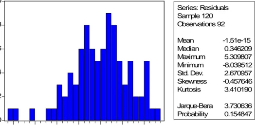
For both of our regression models significant Jarque-Bera statistics were obtained. (see appendix I, tables 7, 8 & 9) We can therefore conclude an acceptance of the null hypothesis, thus the data is normally distributed.
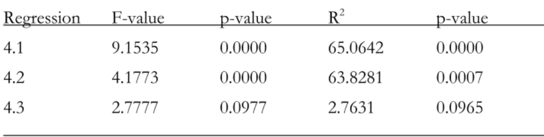
The next vital thing to test is if heteroscedasticity is present in the data. Under the presence of heteroscedasticity the tests will most likely provide inaccurate results due to the fact that the variance of the estimated β will for e.g. become overly large, indicating statistically insignificant coefficient. As a consequence the t-value will be smaller than what is actually true. (Gujarati, 2003) On these grounds White’s General Heteroscedasticity test is performed for all the regressions to assess a possible problem.
H0: No heteroscedasticity
H1: Heteroscedasticity
From the tests we conclude that heteroscedasticity is clearly present in regressions 4.1 and 4.2 by looking at the p-values obtained from the F- and R2 -statistics.
Table 1 – White’s General Heteroscedasticity test
Regression F-value p-value R2 p-value
4.1 9.1535 0.0000 65.0642 0.0000
4.2 4.1773 0.0000 63.8281 0.0007
4.3 2.7777 0.0977 2.7631 0.0965
At the five percent significance level the p-values for regressions 4.1 and 4.2 are statistically significant, and therefore the null hypothesis is rejected. However, adjustment for regression 4.3 is not necessary.
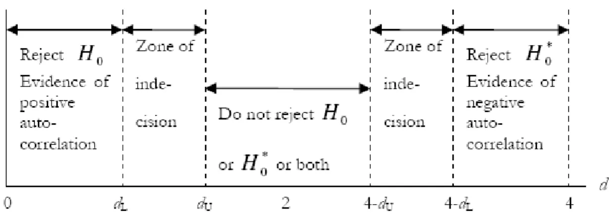
The last problem to check the model for, before obtaining BLUE, is the issue of autocorrelation. If this is the case the usual t and F tests may not be valid. Testing to see if autocorrelation problem exist is done using the Durban-Watson (DW) d test. (Gujarati, 2003) The obtained DW-statistics ends up in the zone of indecision for autocorrelation, for regressions 4.1 and 4.2. On this basis we cannot conclude if there exists autocorrelation in
Empirical Findings
our data or not. (see appendix I for DW-statistics, table 10 and figure 1) Nevertheless, scatter plots of the residuals indicate no problem. (see appendix II, graphs 8 & 9) Therefore we assume that no adjustment is needed for these two regressions. However, 4.3 ends up in the zone for positive autocorrelation, and must be adjusted.
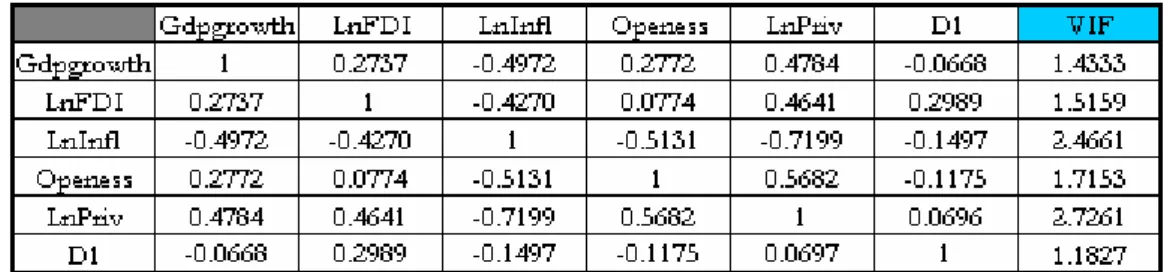
Even though not affecting BLUE, it is also central to rule out multicollineraty as this increase the risk of accepting a false hypothesis, a so called type two error. The problem can be detected by having overall insignificant t-values while at the same time having high R2 or by studying a correlation matrix to see if the independent variables are excessively
correlated against each other. (Gujarati, 2003) Table 2 – Correlation Matrix
From our correlation matrix it is observed that there are some high correlation values between the independent variables, especially for privatization vs. inflation. This indicates multicollinearity, thus further tests is necessary. This can be done by observing the Variance-inflating factor (VIF) were values of 10 indicate severe multicollinearity. However, the VIF statistics for all the variables are significantly lower than 10, indicating that multicollinearity is not a problem in our model.
Since our data suffer from some of the problems that prevent the regressions from being BLUE it is important to interpret the findings in the following section with caution, even though adjustments for heteroscedasticity and autocorrelation will be performed. Hence, if any abnormal results are obtained this might be an indication of distortions in the regressions.
4.4.2 Hypothesis Testing
On the basis of our findings in the previous section (4.4.1), the regressions presented here are all adjusted for either heteroscedasticity and autocorrelation, or both. The adjustment is done through White Heteroskedasticity-Consistent Standard Errors and the Newey-West HAC Standard Errors & covariance for correcting the OLS standard errors (Gujarati, 2003).
Please note before viewing the coefficients that lin-log models are present in regression 4.1 and 4.2. Thus, the interpretation of the results in these two cases will be as stated in equation 4.4, in section 4.4.1.
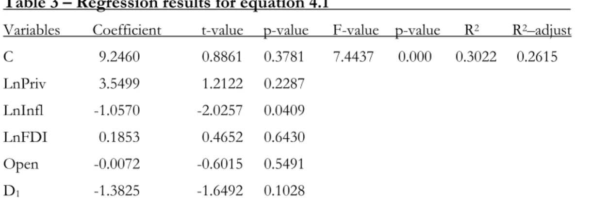
The first equation to test is our main regression model (4.1) to see if there is a statistical difference in the choice of policy and the GDP development
Empirical Findings
From the given equation the following results were extracted. Table 3 – Regression results for equation 4.1
Variables Coefficient t-value p-value F-value p-value R2 R2–adjust
C 9.2460 0.8861 0.3781 7.4437 0.000 0.3022 0.2615 LnPriv 3.5499 1.2122 0.2287 LnInfl -1.0570 -2.0257 0.0409 LnFDI 0.1853 0.4652 0.6430 Open -0.0072 -0.6015 0.5491 D1 -1.3825 -1.6492 0.1028
Dependent Variable: ∆GDP/cap Method: Ordinary Least Squares
Adjusted for heteroscedasticity: White Heteroskedasticity-Consistent Standard Errors & Covariance Included observations: 92 after adjustments
When testing our regression at the five percent significance level the results indicate that policy has no effect on the development of GDP. The reason is that the dummy variable (D1) shows an insignificant value and hence supports an acceptance of our null hypothesis.
Even though the β-coefficient indicate that the shock therapy countries on average have slightly more negative GDP per capita growth than the gradualist countries, this difference is not at all significant. In addition, all variables except for inflation show insignificant values. Thus, this limits us from drawing further conclusions from the obtained results. However, even though all but one variable indicate insignificant values, the F-statistics is significant and hence the variables are significant for the regression. Moreover, it is essential to test how well the model fits the data. This is done by studying the R2 values, the
coefficient of determination, were 1 represents a perfect fit. (Gujarati, 2003) The coefficient of determination in the regression is fairly low, R2 = 0.3022. However, a low R2
does not necessarily imply clear evidence against the model. The theory that rests behind the model is of more importance. Since GDP is a variable that take many things into consideration the independent variables chosen here might not be a fair measurement overall. However, the limitations made were necessary to match the theory and to stress the implications that the two different policies had on GDP per capita growth. (Gujarati, 2003) Given that our dummy variable signal that policy is of no significance in the transition process as a whole we found it is necessary to test the hypothesis on a deeper level. Hence, adding the policy dummy for each of the independent variables as clarified from the regression equation 4.2:
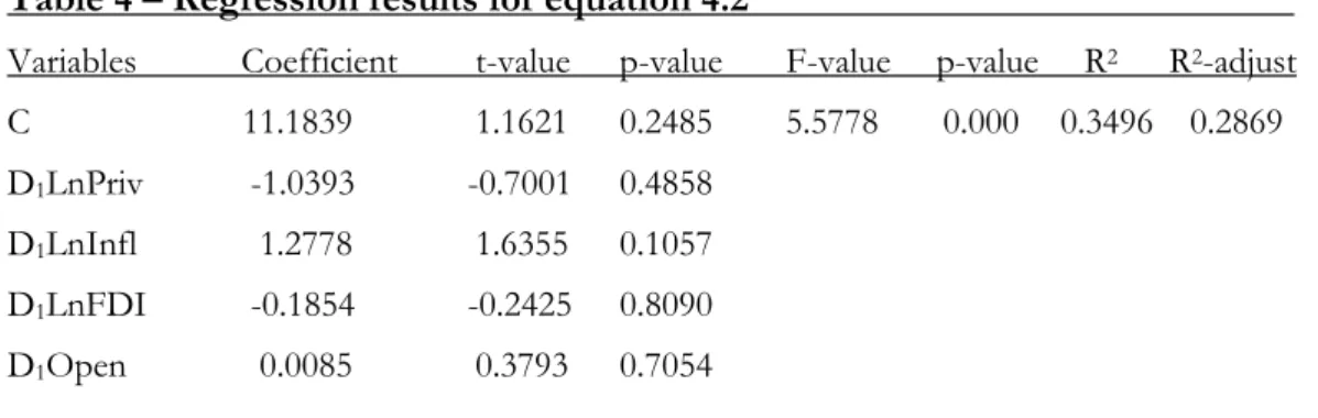
∆Y/Y= β0 + β1 D1 lnP1 + β2 D1γ2 + β3 D1lnπ3 + β4 D1lnλ4 + ε (4.2)
Empirical Findings
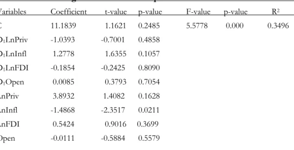
Table 4 – Regression results for equation 4.2
Variables Coefficient t-value p-value F-value p-value R2 R2-adjust
C 11.1839 1.1621 0.2485 5.5778 0.000 0.3496 0.2869 D1LnPriv -1.0393 -0.7001 0.4858
D1LnInfl 1.2778 1.6355 0.1057
D1LnFDI -0.1854 -0.2425 0.8090
D1Open 0.0085 0.3793 0.7054
Dependent Variable: ∆GDP/cap Method: Ordinary Least Squares
Adjusted for heteroscedasticity: White Heteroskedasticity-Consistent Standard Errors & Covariance Included observations: 92 after adjustments
The result that was obtained from equation 4.1 is enhanced through this regression. All of our dummy variables indicate that policy choice has no impact on GDP per capita growth since the p-values are all statistically insignificant at the five percent significance level. Thus, once again the null hypothesis is accepted. All the variables show insignificant values, but the F-statistics is on the other hand significant (for the whole regression result, see appendix I, table 11). Additionally, we have obtained a slightly higher R2- and adjusted R2
values, however this is explained by the inclusion of additional variables.
Since we have obtained two indications to accept the null hypothesis we find it interesting to test if there is a difference between our CEEC and the reference countries in the percentage GDP per capita growth. Hence, the following regression was tested.
∆Y/Y= β0+ β1 D2 + ε (4.3)
Table 5 - Regression results for equation 4.3
Variable Coefficient t-value p-value F-value p-value
C 2.1227 6.3018 0.0000 22.0670 0.0000
D2 1.6935 4.0427 0.0001
Dependent variable: ∆GDP/cap Method: Ordinary Least Squares
Adjusted for Autocorrelation: Newey-West HAC Standard Errors & Covariance Included observations: 147 after adjustments
The results attained show that there is a statistically significant difference between the CEEC and the reference countries. Thus, we have evidence that the average GDP per capita growth is higher for the CEEC than for the reference countries.
This is in line with what one could expect after studying the Solow-Swan growth model, a neoclassical growth model. The stated growth model describes that the capital-output ratio is precisely the adjusting variable that would lead a system back to its steady-state growth path. Hence, the Solow-Swan model describes absolute convergence between countries with different initial standard of living levels if they have access to the same technology, and experience the same savings rates and population growth. (Dornbusch, Fischer & Startz, 2004)
Empirical Findings
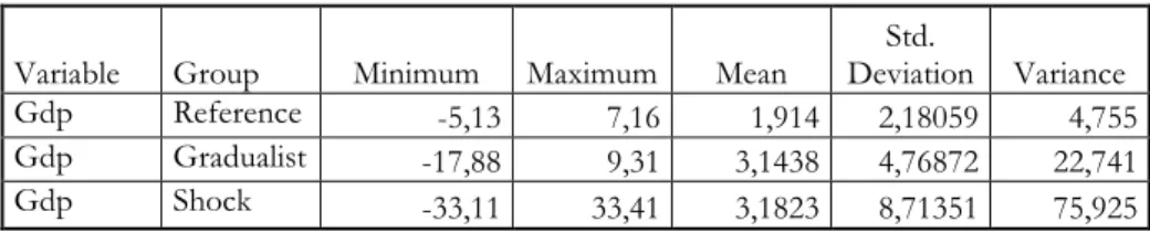
These results are strengthen further by looking at table 6 where the mean value for GDP reveal that there is a small difference between our two transition models, but a high deviation between the CEEC and the reference countries.
Table 6 – Descriptive statistics of GDP between the groups
Variable Group Minimum Maximum Mean
Std.
Deviation Variance Gdp Reference -5,13 7,16 1,914 2,18059 4,755 Gdp Gradualist -17,88 9,31 3,1438 4,76872 22,741 Gdp Shock -33,11 33,41 3,1823 8,71351 75,925
To conclude this section the following findings have been made:
The chosen policy in itself does not have an overall effect on GDP per capita growth. This is based on the acceptance of our main null hypothesis from regression 4.1, where the policy dummy variable gave an insignificant value. However, in relation to the acceptance of the null hypothesis, the independent variables were all estimated with the policy dummy added in regressions 4.2. The findings obtained concur with the findings obtained from regression 4.1. On this basis we have clear evidence pointing in the direction that the chosen transformation policy itself does not have an impact on GDP per capita growth. Nevertheless, when testing if there exist a difference in the GDP per capita development between all of the chosen CEEC and the reference countries, the findings were significant. Hence, the CEEC has experienced a more rapid GDP growth during the 12 year period. Lastly, since both regression 4.1 and 4.2 support each other and indicate an acceptance of our hypothesis and no other abnormal result have been found, the risk that the regressions have been distorted due to any problem mentioned in section 4.4.1 is low.
Analysis
5
Analysis
The following section analyses the results that were presented in the previous sections in an attempt to tie the given results to the thesis’s theoretical framework.
Through the acceptance of the null hypothesis we are concluding that the choice of transition policy have no impact on the GDP per capita growth for the CEEC. Thus, it seems like there are other factors which affect the possible success or failure of the transition. By studying the graphical analysis section (4.1) we see that there especially within the macro-economic stabilization area, measured in the form of inflation, exist vastly different preconditions between the two groups when entering the transition process. The significance of inflation is further enhanced by the empirical finding were regression 4.1 indicated only one significant variable; the inflation rate. Consequently, the inflation variable is highly significant for the GDP development in these transition economies Economist, such as Jeffrey Sachs (1997a) and John Marangos (2005) believe that fighting inflation fast was of the greatest importance for these countries. Correspondingly, the CEEC managed to do so fairly fast regardless of what policy that was used. This is supported by insignificant result for the inflation policy dummy in regression 4.2. Hence, it seems like preconditions of the economy prior to the transition seem to have played a greater part in how these countries GDP per capita growth rate have been affected.
When then studying the results of the insignificant independent variables it can first be concluded that FDI have increased significantly in the CEEC during the measured 12 year period (see graph 4, in section 3.1). In recent years this has especially been noticeable in the shock therapy countries, much due to their sell-out of domestic companies during the privatization process to foreign investors. The empirical findings indicate a positive contribution of FDI upon GDP growth, however as just stated above this finding is insignificant. On this basis no further conclusion can be drawn for this variable.
However, the empirical results indicate the possible downside of too high levels of FDI in a country. Many times high levels of FDI cause a negative relation to the trade sector in relation to GDP. Leading to the fact that the trade balance will be negative, with a surplus of imports. Therefore, the openness variable will have a negative relation to GDP. This is what the regression’s insignificant result for equation 4.1 and 4.2 indicate. However, there is still no significant difference between the two groups. The last independent variable in our regression model is privatization. The graphical analysis from section 3.1, table 7 illustrates that there is no difference between the two policies. The graphical illustration is further supported by the regression results of 4.2, that show that policy choice have no affect on this variable either.
To combine our findings with earlier conducted studies we would first like to once again inform you that there are researchers that have given support to all three angles of this problem. Sachs (1997 a & b) claim that the shock therapy model is the best way to undergo the transformation while Blanchard (Aghion & Blanchard, 1994) states the gradualist policy is the best model. However, there is also a third group of advocates; those that claim that the choice of policy has no impact on GDP per capita growth. Thus, on the basis of our empirical findings and the acceptance of the null hypothesis we agree with the third group of researchers. Among these scholars is, Jürgen Beyer (2001) from the Max Planck Institute in Cologne. Beyer (ibid) claim on the basis of his conducted empirical research that the policy choice when transforming an economy into a market economy is of little