Cyclical consumption and the aggregate stock market: Evidence from the Nordic countries

(1)

Cyclical consumption and the aggregate

stock market:

Evidence from the Nordic countries

MASTER THESIS WITHIN: Business Administration NUMBER OF CREDITS: 15 Credits

PROGRAMME OF STUDY: International Financial Analysis

AUTHOR: Sasu Elmeri Huttunen and Govert Mattheus Looije

(2)

Master Thesis in Business Administration

Title: Cyclical consumption and the aggregate stock market: Evidence from the Nordic countries

Authors: S.E. Huttunen and G.M. Looije

Tutor: D. Schäfer

Date: 2021-05-24

Key terms: Cyclical consumption, Aggregate stock market, Nordic countries, Out-of-Sample Predictability

Abstract

Researchers have dedicated considerable work to explaining components to excess stock market returns. Recently, Atanasov et al. (2020) managed to explain some of this variance in the US stock markets with a cyclical consumption variable. We have applied their model into the Nordic countries and compared it to a second model containing additional control variables. From the analysis, we find that cyclical consumption is able to explain excess stock market returns across five different h-quarter ahead excess returns. However, results are not consistent across countries. The extended model improves the explanatory capabilities of the model only up to two-year ahead excess returns. The cyclical consumption measure is also able to predict excess returns better than an historical average model. The findings in this paper are robust to out-of-sample predictability analysis and to a different measure of consumption and returns.

(3)

List of tables

Figure 1 - Measuring cyclical consumption (Atanasov et al., 2020) ... 8

Figure 2 - Regression model for stock return predictability (Atanasov et al., 2020) ... 8

(5)

Figure 4: Cyclical Consumption Nordic Countries ... 21

Table 1 - Sample period for each country ... 25

Table 2 - Descriptive statistics ... 27

Table 3 - Correlation matrices ... 29

Table 4 - Regressions Denmark ... 33

Table 5 - Regressions Finland... 35

Table 6 - Regressions Norway ... 37

Table 7 - Regressions Sweden ... 39

Table 8 - Likelihood Ratio test ... 41

Table 9 - Wald test ... 42

Table 10 - Out of Sample regressions ... 45

Table 11 - Alternative return measure ... 48

Table 12 - Alternative consumption measure ... 49

(6)

1. Introduction

Over the years researchers have made a considerable effort into finding explanations for e.g., changes in stock prices, predictability in stock prices or the high equity premium. However, regardless of these efforts, the findings are still somewhat unclear. For example, as briefly mentioned in Guo (2006), several macroeconomic variables have been shown to determine excess returns in the market. However, Guo (2006) notes the beforementioned relationship between macroeconomic variables and excess stock returns are not as strong in the out-of-sample data. One of the more prominent studies in this field is Fama and French (1989), who find that the risk premium (i.e., excess return) follows the same trend as the business cycle. They conclude that the expected returns of stocks are negatively related to the economic environment. This conclusion is relevant for this research project since it shows that relatively straightforward explanations such as e.g., firm size are not the only relevant explanations. The focus of our research is on consumption, or more specifically, the relationship between the newly developed cyclical consumption measure introduced by Atanasov, Møller and Priestley (2020) and excess stock market returns. As mentioned before several studies have been dedicated to find the effects of macroeconomic shocks on excepted stock returns. Fama and French (1989) find that excess returns are negatively related to macroeconomic variables (i.e., economic environment). Ang and Bekaert (2007) find that dividend yields predict excess returns on stocks when analysed on the short time horizon. Guo (2004) uses a consumption-based model that can be used to explain the equity premium that is generally found in research. Lettau and Ludvigson (2001) find that the consumption-wealth ratio is positively related to future stock returns and excess returns. However, one criticism as outlined by e.g., Bossaerts and Hillion (1999) is that the out-of-sample predictability of most of these macroeconomic variables is negligible1.

Aggregate consumption in an economy can be linked to two broad states of the overall economy: the good state (i.e., expansion) and the bad state (i.e., recession). A recession is traditionally seen as a state where economic activity is declining. Indicators for this decline are e.g., production, employment and real income. An increase in these same factors in an indication of a state of expansion (Berge and Jorda, 2011). Atanasov et al. (2020) showed that

1_{Where out-of-sample analysis refers to the method of comparing actual data with data predicted with the}

(7)

cyclical consumption can be used as a predictor for future aggregate stock returns. The authors explain this finding with the change in the marginal utility for consumption. When the aggregate consumption within a market falls, the future expected stock returns rise due to enhanced marginal utility for consumption. The authors were able to show that this works inversely as well: when aggregate consumption rises, the marginal utility for consumption decreases and therefore, the future expected aggregate stock returns fall.

The purpose of this paper is to find out whether the cyclical consumption model of Atanasov et al. (2020) has predictive power over excess stock market returns when applied to the Nordic countries and whether the model can be improved by adding additional macroeconomic predictor variables. We test this by performing two different regressions. After these regressions, we conduct a Likelihood Ratio test and a Wald test to see if the addition of the control variables improves the model. Results from the base regression model indicate that cyclical consumption is able to predict excess stock market returns at least one-quarter ahead for all countries. However, if the prediction horizon increases, the results become less consistent across countries (i.e., some countries display an insignificant relationship). These results contradict the conclusions made by Atanasov et al. (2020), who find a significant relationship consistently (i.e., for every prediction horizon) for the US market. For the extended model we find that cyclical consumption is still able to predict excess stock market returns one-quarter ahead, but it is rarely able to predict excess returns at longer prediction horizons. The results of the base model are robust to testing for their out-of-sample predictability, to a different measure of returns and to a different measure of consumption.

Movements in the stock markets are considered arbitrary or ambiguous at the least. The causal relationships leading to the stock market movements are one of the most studied subjects within finance, yet results are still not conclusive. Since Atanasov et al. (2020) managed to show the value of cyclical consumption in predicting excess stock market returns, a task which has been unsuccessfully tried numerous times, it is essential for future studies related to the financial markets to see if this relationship holds outside the United States. Additionally, since the cyclical consumption variable is newly developed, it has not yet been studied extensively. This thesis will add to the limited academic literature that uses this new variable.

This paper is divided into several different sections. Chapter two provides a literature review, firstly looking at the Atanasov et al. (2020) paper in more detail and summarize their findings and methodology. It will be followed with a section on the problems related to the use of single

(8)

variable models. In the last section of the literature review, we will review the literature on the additional variables that are to be added into our model. Chapter three goes over the methodology (i.e., presenting the regression model) used in this research, which includes variable definitions and calculations. Following the variable definition, we present the data sources and the final sample period for each country. Chapter four presents the results of the two regressions for each country. Chapter five and six present the results of the out-of-sample analysis and additional tests, respectively. Chapter seven provides a conclusion and possible avenues for future research.

2. Literature Review

In this section of the paper, we firstly review the recent paper by Atanasov et al. (2020) in which the cyclical consumption variable is introduced. Secondly, we present some of the issues that are related to single-variable regression models. Finally, we go through literature on the additional variables we have chosen to include in the following order: oil prices, GDP growth, government bonds and inflation.

2.1 Cyclical Consumption and Stock Returns

Past research has mainly focused on the effect of aggregate consumption on the predictability of stock returns, which is discussed in more detail later. Atanasov et al. (2020) use a method proposed by Hamilton (2018) to extract that cyclical component of consumption. This procedure produces, among other things, a variable that captures macroeconomic trends and fluctuations. One of the general theoretical explanation for the time-variance in the stock returns is external habit formation by the agents in the market. Several papers have found that habits follow the same trend as consumption. The Atanasov et al. (2020) paper provides us with several interesting findings which might improve future research of consumption. The effect of macroeconomic shocks on the expected stock returns has been extensively studied. The general finding is that there is a negative relationship between consumption and future stock returns (e.g., an increase in consumption leads to a decrease in stock returns). The

(9)

exact mechanism between these two variables will be explained in a later paragraph. However, this previous research generally finds that the macroeconomic shocks (i.e., macroeconomic predictors) are only able to predict stock returns in good times. This is where the cyclical consumption variable can play an important role. Atanasov et al. (2020) argue that the cyclical consumption variable can be used to extrapolate whether an economy is experiencing good or bad times. They propose a negative relationship between the cyclical component of consumption and future stock returns. However, this result should be present in both good and bad times, contrary to the negative relationship between aggregate consumption and stock returns that is generally only found in good times.

Atanasov et al. (2020) use a linear projection method, which was introduced by Hamilton (2018). The cyclical consumption variable is found by taking the error term of the following equation:

Figure 1 - Measuring cyclical consumption (Atanasov et al., 2020)

The use of lagged consumption variables, as shown by 𝑐_𝑡−𝑘, allows us to extrapolate a variable that is actually related to economic fluctuations (i.e., consumption changes over time, depending on the economic state). This is the cyclical consumption variable, which is equal to the value of 𝜔_𝑡 in Figure 1. Although out of the scope of this thesis, Atanasov et al. (2020) provide a graph which shows the trend of the cyclical consumption variable in the US along with the ‘official dates’ of recessions and this graph indeed shows that the cyclical consumption drops in the recession years and rises after said recessions, thus providing evidence that this variable follows the real economic situation.

To test the predictive power of this new variable on future stock returns, they use the following model:

(10)

where 𝑐𝑐_𝑡 corresponds to the 𝜔_𝑡 from Figure 1 (i.e., 𝑐𝑐_𝑡 is the residual from the regression in Figure 1). They run this regression of excess returns for several different values of h (i.e., quarters in the future) and find that the cyclical consumption negatively predicts future stock returns at a significant level, and this is seen for every value of h. To outline one specific finding, they find that a one standard deviation decrease in cyclical consumption leads to an increase of around five or six percentage point in the annual return. These results show that the beforementioned expected effect of economic downturn on future stock returns (i.e., an increase in returns) is also found when using the cyclical consumption variable. This relationship holds over several different time horizons.

Previous studies that look at the predictability of future stock returns have had one common problem that relates to the effect of crises, namely, asset pricing models are generally only able to find a relationship between popular predictor variables and future stock returns during bad times (i.e., a recession) and not during good times (i.e., business cycle expansion). The cyclical consumption variable is supposedly able to tackle this problem. To test whether this is indeed the case, Atanasov et al. (2020) add a state indicating variable, which is used to define a recession (or expansion). For robustness, they use several different ways of defining a recession (e.g., GDP growth). Using this state variable, they are able to test the effect of the cyclical consumption on future stock returns in both good and bad times. They manage to confirm that the cyclical consumption variable is able to predict future stock returns in both good and bad times, regardless of the time horizon. This implies that this new variable is an improvement on previously studied macroeconomic predictor variables.

To conclude this discussion, we will summarize several of the different points made in the paper that were outside the scope of this thesis and the conclusion provided by Atanasov et al. (2020). They perform several robustness tests to find out whether their findings hold in several different situations. Firstly, they test the out-of-sample predictive power of the newly developed measure. Secondly, they construct the cyclical component from several different consumption expenditures (e.g., non-durable goods consumption) and test their predictive power. Thirdly, they test the relationship between cyclical consumption and stock returns in an international setting (i.e., they measure returns by looking at the MSCI World and other local indices). Fourthly, and finally, they compare the out-of-sample R-squared of 19 popular predictor variables for future stock returns. The main conclusion of the paper is that the newly developed variable can predict future stock returns in both good and bad times. The ability to have predictive power in both good and bad times is an improvement on the most popular

(11)

predictive variables commonly used in research. Their findings are in line with rational asset pricing theory (i.e., agents take the business cycle conditions into account). Additionally, the robustness tests mentioned before, provide evidence that the cyclical consumption variable is better able to predict future stock returns compared to other commonly used measures. Although not mentioned in their paper, the relationship outlined by Atanasov et al. (2020) is related to a mechanism found by Yogo (2006), who attributed cross-sectional variation in stock returns and countercyclical variation in equity risk premium to consumption. He argued that durable consumption falls during recessions, which leads to consumption utility rising. As marginal utility for consumption rises, stock returns are low. Therefore, investors require high expected returns to hold the stocks. Durable consumption is defined as the purchase of goods and services that provide service flows and utility for more than one period. Similarly, nondurable goods are exhausted at the moment of purchase. This supports the theory that a decline in aggregate consumption leads to higher utility of consumption and future expected stock returns (Atanasov et al., 2020).

Based on earlier research, consumption is generally believed to follow the concept of habit formation. Habit formation, as described by Campbell and Cochrane (1999), implies that if an agent (i.e., the consumer) is exposed to a certain stimulus for a continuous amount of time, the effect of said stimulus deteriorates over time. They note that the level of habit of an agent depends on the aggregate consumption in the market, not its own individual level of consumption (i.e., external habit formation). Using this external habit formation concept, they apply it to certain stock market effects. The main finding in their paper, which is also the core of the relationships at hand, is that their consumption-based model is able to capture certain behaviour shown by the stock market. For example, they find that expected returns, and volatility of these returns, are high when the aggregate consumption falls. They posit that this is due to (1) economic growth, and fluctuations therein, are associated with certain welfare costs (i.e., higher welfare costs lead to consumers requiring higher returns) and (2) the concept of precautionary savings effect, i.e., the theory that agents save more and consume less to prepare for an expected economic downturn (Skinner, 1988), which is able to offset the intertemporal substitution effect. These two points are important to acknowledge, since this directly ties to the risk-aversion of the individuals, i.e., people are afraid of an economic downturn, which is the risk, they will save more and consume less. Campbell and Cochrane (1999) also note that in general, when the surplus consumption ratio is low, an individual experiences high levels of risk aversion. These findings provide us with the mechanism that

(12)

drives the relationship between consumption and stock returns. Low consumption generally indicates a high level of risk-aversion which makes investors to require high returns. Additionally, the stock market has to offer sufficient returns to prevent consumers from making precautionary savings. The explanation of risk-aversion and other investor biases have been shown to be some of the drivers behind the equity premium puzzle (e.g., Ang, Bakaert and Liu, 2005 & Fielding and Stracca, 2007).

2.2 Concern over single variable regression models

Rapach, Strauss and Zhou (2009) explored equity premium predictions by expanding on the previous work by Welch and Goyal (2008), who showed that individual economic variables do not deliver predictive power to equity premium in both the sample period and the out-of-sample period. This was done with a simple regression model as seen below, where 𝑟𝑡+1 is the excess return on the markets and 𝑥_𝑖,𝑡 represents a vector of individual economic variables (e.g., yield spread and inflation).

Figure 3 - Standard regression model for equity premia (Rapach, Strauss and Zhou, 2009)

Rapach et al. (2009) expanded on the work of Welch and Goyal (2008) by combining some of the individual regressors into the same multivariate regression model. The results show that these combined economic predictor variable models significantly reduce the volatility in the expected equity premium forecasts, both for the sample and the out-of-sample periods. The new models were also able to work better during extreme economic conditions, especially in the downturns. Furthermore, some important observations are made. Firstly, required risk premia increase during economic recessions. Secondly, the same multivariate models used to predict equity premium can also be used to forecast some macroeconomic variables such as real GDP growth or real earnings growth. In conclusion, using these so-called combination models gives better predictions for both expected equity premiums and macroeconomic conditions than the regression models relying on a single variable, which tend to be highly volatile. Furthermore, for many sample periods, the combination models were better at predicting excess returns than the historical average, which presents a strong case for the

(13)

discussion of predicting equity premiums. These conclusions raise doubts on the efficiency of the cyclical consumption model by Atanasov et al. (2020), who use only one explanatory variable. According to the findings of this paper, the single regression model could potentially gain explanatory and predictive power when other explanatory variables are added to the model.

2.3 Additional Control Variables

In their paper, Atanasov et al. (2020) tested various alternative predictor variables to see how the cyclical consumption variable matches against some of the more traditional predictor variables. We have chosen to add some of these other variables into our extended model to see if it improves the predictive power of the model. In this section of the paper, we will go through several variables generally found in literature to be able to explain and/or predict excess returns, namely: an oil price variable, a GDP growth variable, a risk-free rate variable, a long-term interest variable and an inflation variable. We subsequently summarize some of the previous findings on the usefulness of the aforementioned variables in predicting asset returns.

2.3.1 Oil Prices

Wang, Wu and Yang (2013) describe the relationship between oil prices and stock markets to be of great interest among economists. In their research, they divide the data sample into oil exporting and oil importing countries. For each country, the index of their respective stock markets is used to observe the effects of oil price changes. Oil prices were based on the West Texas Intermediate crude oil, which is a commonly used proxy for oil prices. The authors find a linear relationship between oil prices and stock market returns. Furthermore, it is established that the difference between being an oil importing or oil exporting country affects the extent, duration and the direction of the relationship between oil prices and stock market returns. The research yields many implications as to the effects of oil prices on the stock market. Firstly, linear models manage to show a relationship between changes in oil prices and stock market returns. Secondly, the effects on the stock markets are dependent on whether the sample country is mainly an oil importer or exporter. Furthermore, the predictive power of oil price change variable is greater for oil-exporting countries and depends on the importance of oil for the respective country. Thirdly, the increases in demand for oil leads to enhanced covariance

(14)

between oil prices and stock market returns. Based on this research we believe that adding oil price index variable into our model is likely to improve the predictive power compared to the base model.

Driesprong et al. (2008) provide us with further confidence on adding an oil price variable in the model. The authors studied the predictability of stock market returns using changes in oil prices, both in developed and emerging markets. They used monthly data spanning from 1973 to 2003 for 48 countries. For the crude oil prices, they use three proxies: Brent, West Texas Intermediate and Dubai. Some spot and future crude oil prices were also utilized. The paper manages to confirm that changes in oil prices contain predictive power on stock returns and this relationship is stronger in developed countries than emerging markets. Increases in oil prices result in lower stock returns and decreases in oil prices lead to higher stock returns in the following month. Furthermore, the authors find evidence for underreaction by the investors; on average it takes six trading days before the changes in oil prices are captured in the stock prices. This is attributed to gradual information diffusion hypothesis, stating that when assessing the impact of oil price changes into the stock markets is difficult for investors, they may underreact or do so at varying time points. Supporting this argument, the authors find that when introducing lags in the model, the model becomes stronger. This phenomenon is even stronger in market sectors where it is harder to interpret the effects of oil price changes. This paper gives us further confidence in adding oil price variable into the base model.

2.3.2 GDP growth

Vassalou (2003) created a model that used expected GDP growth variable to predict cross-sectional equity returns. Previously, research has commonly used either the CAPM or the Fama-French model when attempting to predict asset returns. Fama-French model considers market factors high-minus-low (HML), which measures the book-to-market ratio and small-minus-big (SMB), which measures the size factor. These factors proxy some of the undiversifiable risk in the markets, such as the default risk. However, the factors are believed to capture information on equity returns besides the default risk. The author suggests that they may contain information on risks connected to macroeconomic variables. The research seeks to discover the driving forces behind HML and SMB. The author uses news related to the future GDP growth as a proxy for expected GDP growth. The sample data used in the was quarterly equity portfolio data and 30-day T-bill rates spanning from 1/1952 to 12/1998. It is found that

(15)

the new variable is able to predict some of the variation in cross-sectional asset returns. When adding the variable into the CAPM, the predictive power was significantly enhanced. Furthermore, when adding the variable into the Fama-French model, the SMB and HML factors become obsolete. Based on this, we find adding some form of expected GDP growth variable to our model to be worthwhile. However, their sample time period is very different from ours, so the predictive power might not be as significant. Lastly, their sample country was the US, which contains different economic characteristics compared to the Nordic countries in our sample.

Following the findings of Vassalou (2003), Nguyen et al. (2009) studied whether using the future GDP growth factor variable makes the SMB and HML factors of the Fama-French model obsolete in their sample country Australia. Since Australia possesses a considerably stronger connection between the SML and HML factors to asset returns than the US, this study gives indication on whether the findings of Vassalou (2003) are generalizable. The authors follow the methods of the base paper: they create a mimicking portfolio to catch the news about expected GDP growth. They use the monthly data from the Australian Securities Exchange for time period 1990 to 2005. Then they attempt to see whether the expected GDP growth variable covers some of the equity returns. The variable is then added to the Fama-French model to see if there are improvements and if the Fama-French factors lose their ability to bring more predictive power. The authors find that the expected GDP factor does not contain explanatory power over equity returns. Furthermore, they confirm that in their sample, adding the GDP growth factor did not reduce the significance of the SML and HML factors when added into the Fama-French model. These results indicate that the Fama-French variables do not proxy the market risk related to future GDP growth. The authors believe that this is due to Australia presenting a weak correlation between GDP and Fama-French factors. Based on these findings, we question whether adding the expected GDP growth variable is able to bring more value to our model than simply using Fama-French model instead. However. since we do not know the correlation between SML and HML to GDP in our sample countries we believe it to be worthwhile to add GDP growth to our model.

2.3.3 Risk-Free Rate (short and long-term government bonds)

The capital asset pricing model (henceforth CAPM) is a widely used model to evaluate stock returns. It contains a variable we think would improve our model: the risk-free rate. Its

(16)

relationship with stock returns has been studied extensively (Andersson et al, 2017; Shiller and Beltratti, 1992; Konstantinov and Rusev, 2020). Mukherji (2011) wrote about the market risk and the inflation risk of Treasure bills with different maturities, as they are commonly used as a proxy for the risk-free rate. The time to maturity on the government bonds determines the yield for the investor, meaning that in general, long-term bonds with the same default risk as the short-term bonds provide a higher yield. However, it has been previously established that long-term Treasury bonds contain positive market betas, exposing them to some market risk. To compare the difference in the effect on the CAPM model of long and short-term Treasury bonds, the author uses monthly return data from 1926 to 2007 for short, intermediate and long-term Treasury bonds. He uses the S&P 500 as a proxy for the market portfolio. The paper shows that volatility, real returns, inflation and market risk increase along with the time to maturity of the bond. For one and five-year bonds, the market risk is very low and while all bonds, regardless of their maturity terms, contain inflation risk with it being the lowest for one-year T-bills. Based on these results, we are compelled to add short-term Treasury bonds to our list of predictor variables as a proxy for the risk-free rate. Following the findings of Ang and Bekaert (2007), we expect to find a negative relationship between the short-term interest rates and market excess returns.

Shiller and Beltratti (1992) assumed there exists a negative relationship between changes in stock prices and changes in long-term bond yields. The authors reason that, if the expected yields on long-term bonds increase, the bonds become a relatively more competitive asset, and lead to a decrease in stock prices. The authors test the existence of the hypothesised relationship using data from both the US and the United Kingdom over an extensive time period. Their results indicate that there is in fact a significant negative relationship in both sample countries, in which the UK showed a more distinct negative relationship. Although the paper does not show which market affects which (i.e., the direction of causality), the findings suggest an overreaction from the stock markets over changes in the bond markets. While the authors are unable to rule out the possibility of this negative relationship being the product of the inflation expectations of investors, they are able rule out that it is caused by actual. They find that in both sample countries, the relationship between changes in bond yields and changes in actual inflation is not very strong. There are a few considerable reasons why we are not yet convinced to add a variable capturing changes in long-term interest rates into our predictive model. Firstly, the sample countries are culturally and economically different from our respective sample

(17)

countries. Secondly, although the time period considered in the paper is extensive, it is somewhat outdated, as the latest observation in their dataset comes from the year 1989. Using the long-term interest rate in our model may not be as straightforward as implied since studies have shown that the relationship between stock and bond prices is not constant (Capiello et al., 2006; Connolly et al., 2005) and in some cases, may even change sign to negative (Gulko, 2002). Andersson et al. (2008) studied the causalities of this time-varying relationship. One of the considered influencers is inflation; since the increases in expected inflation will raise the discount rates, bond prices should go down. The other considered explanatory variable is perceived market uncertainty; if the investors find the markets to be in a volatile state, they will require a higher risk premium to hold on to their stocks, compared to less risky assets such as bonds. Furthermore, the investors might lean towards bond markets to reduce their portfolio volatility.

Connolly, Stivers and Sun (2005) studied the daily covariance between stock and Treasury bond returns. The authors were especially interested in further explaining the occurrence of periods where the relationship between the two asset types turns negative from its usual positive relationship. In particular, they investigated whether stock market uncertainty could be behind the change in stock-bond return relationship. They use US data of the stock and Treasury bond returns within the time period 1986-2000. Based on past literature, they choose implied volatility and abnormal stock turnover as the proxies for stock market uncertainty. Implied volatility is meant to reflect uncertainty about the future stock volatility and abnormal stock turnover is expected to mirror changes in the investment opportunity set. The authors establish some implications on the stock-bond return relationship. Firstly, there is indeed a negative correlation between the two uncertainty proxies and stock-bond return relationship. This means that when stock market uncertainty increases, there is subsequently a higher chance of observing a negative stock-bond relationship during the following month. Secondly, bond returns tend to be high, relative to stocks, when implied volatility of the stocks increases and vice versa. Based on this research we would assume that as the market uncertainty increases due to e.g., recession, Treasury bonds can be used to predict the negative change in the stock returns, which potentially improves our model.

(18)

2.3.4 Inflation

The connection between inflation and stock market returns is a well-researched topic. Fama and Schwert (1977) wrote a paper on asset returns and inflation. They used the Consumer Price Index (CPI) to measure the rate of inflation, for a sample period from 1953 to 1971. A variety of assets were used to compare CPI to the returns. The authors used New York Stock Exchange for common stocks, T-Bills with 1-6 months maturity for short-term bond asset returns, US government bonds with 1-5 years maturity time for long-term bond asset returns and finally, Home Price Index to measure the real estate asset returns. It is found that out of all the assets considered in the research, only the real estate asset proxy provides hedge against the two types of inflation: expected and unexpected. This practically means that the nominal real estate returns move tightly together with the inflation rate. In their sample, short- and long-term government bond returns move together only with the expected component of the inflation rate. Furthermore, it is found that returns for common stocks have negative relationship with unexpected inflation rate that changes to a positive sign when it comes to expected inflation rate. As our own paper attempts to provide explanatory model for common stocks, based on this paper, adding inflation variable might be risky. However, as we have already chosen to include Government Bonds as a predictor variable, based on this paper, it might already be captured by the expected rate of inflation.

As to more recent literature on the use of inflation in predicting stock market returns, Engsted and Tanggaard (2002) studied the relation between asset returns and inflation for short- and long-term time periods. The authors investigate aforementioned relation with both US and Danish data. To overcome non-stationarity problem, they apply a VAR model for individual time periods to receive stationary multi-period data. For the US, S&Ps Composite Stock Price Index is used for stock returns and long-term government bonds measure the bond returns. Inflation is measured from the Consumer Price Index, for the sample period 1926-1997. For Denmark, Danish stock market data is used for stock returns and long-term bond returns for bond returns. Inflation is measured from the GDP deflator. The time period for the data is 1922-1996. The previous theories on the relationship lean towards the Fisher hypothesis, according to which the expected nominal asset returns should have covariance of around one with expected inflation. Following this theory, real returns on assets such as stocks should work as a hedge against unexpected inflation and on the contrary, nominal returns, such as coupons on a bond, do not offer such hedge. This theory has been disputed by past research, which has claimed that short-term nominal returns are uncorrelated to inflation. The authors find that for

(19)

the US stocks, the correlation between expected inflation and expected stock returns diminishes when the time horizon is increased, going against the Fisher hypothesis. For US bonds, the correlation with expected inflation is high, but only with long time horizons. For Denmark, the stock return-inflation relationship strengthens with longer time horizons. Expected bond returns have a weak correlation with inflation, and it continues to weaken when moving to longer time horizons. Based on this research, we are expecting that adding an expected inflation variable to our model will bring some predictive power, especially as we consider longer time horizons.

Barnes et. Al (1999) studied whether there exists an inverse relationship between inflation and asset returns, both real and nominal. Previously it has been implied that high inflation is precedes lower real asset returns. This has been hypothesized to be due to informational asymmetries in credit markets, which has subsequent effects into capital structures and financial markets. The authors test the inflation-asset return relationship using data sample of 25 countries for the time period 1957-1996. Firstly, the authors find that the nominal return on equity is negatively correlated with inflation for most of the countries in the sample. The few countries that exhibit a statistically significant positive inflation-nominal asset return relationship are also the countries with highest inflation rates. This is explained to be due to the fact that increases in inflation have diminishing marginal effects on asset returns. Relating to our own research, we observe that Finland, Norway and Sweden are included into the sample and that all of them exhibit the negative coefficient associated with the inflation-equity return relationship. We assume that to be the case for the rest of our sample countries, since they display similar rates of inflation, because a positive relationship is more uncommon and because of similar macroeconomic conditions. In conclusion, we expect that adding an inflation variable will show a slight negative relationship with the stock market returns when we run our tests.

2.3.5 Summary of previous literature

Atanasov et al. (2020) applied a new linear projection method to test whether cyclical consumption can be used in order to predict excess stock market returns. They manage to confirm a countercyclical relationship between cyclical consumption and the excess returns. They improved from the past research by managing to establish a countercyclical relationship which holds both in economic expansions and recessions. However, Rapach et al. (2009) show

(20)

that single variable regression models have some inherent shortcomings. They find that, when multiple variables are combined into a model, the volatility is reduced both for sample and out-of-sample periods. Furthermore, the method of combining several models has been shown to predict excess returns better. We argue that the regression model, as used by Atanasov et al. (2020), can therefore be expanded and possibly improved by adding some additional predictor variables commonly found in literature. These variables include GDP growth, oil price growth, inflation, risk free rates (i.e., short-term government bonds) and long-term government bonds. Literature on GDP growth is somewhat mixed. The variable has potential to predict excess returns, but it might become obsolete when other variables, such as the Fama-French factors are included. The literature on the oil price variable shows us that changes in oil prices are captured in stock prices and that the effect is stronger for countries more dependent on oil (e.g., oil importing vs. oil exporting countries). Literature on inflation says that, in some of the Nordic countries (e.g., Finland and Norway), there is a negative relationship between inflation and equity returns. The short-term government bonds are said to be a suitable proxy for the risk-free rate. Additionally, we included the long-term bonds into our list of variables. It is said that the stock-bond return relationship is usually positive but can turn to negative due to market uncertainty. This argument holds for both short- and long-term government bonds.

Overall, we expect that the addition of the additional predictor variables will improve the model. However, since the regressions performed in this thesis are related to several different quarter-ahead excess returns, we can5not make predictions for the longer quarter-ahead excess returns.

3. Methodology

We start by going through the mechanics of the basic regression model followed by outlining the development of the cyclical consumption variable and excess returns. Secondly, we provide explanation on the development of the control variables, including the expected sign of each control variable. Finally, we summarize the steps needed to obtain the final sample size.

(21)

3.1 Basic regression model

In order to test the relationship between the newly developed cyclical consumption measure and the aggregate stock market returns, we follow the regression model as proposed by Atanasov et al. (2020). However, in order to pin down the effect of cyclical consumption on the aggregate stock market excess returns in the presence of other macroeconomic variables we add to their base model with the macroeconomic control variables outlined in the literature review. The final regression model, with the addition of the control variables, looks as follows:

𝑟𝑡,𝑡+ℎ= 𝛼 + 𝛽1𝑐𝑐𝑡+ 𝛽2𝑉𝑡+ 𝜀𝑡,𝑡+ℎ

where rt,t+h is the aggregate stock market continuously compounded excess return h-quarters in the future, cct is the measure of cyclical consumption lagged one-quarter and Vt is a collection term for all of the control variables included in the model. The exact construction of each of these variables is outlined in the following paragraphs.

3.2 Cyclical consumption

The construction of the consumption measure of focus in this paper is obtained following the Atanasov et al. (2020) paper. They apply a linear projection method by Hamilton (2018) which allows us to extract the cyclical component of a variable (i.e., in this case consumption). For the consumption measure 𝑐_𝑡 we use the log of per capita household consumption of non-durable goods and services, which are seasonally adjusted and at fixed values (i.e., linked to a certain reference year).

In order to obtain the cyclical component, we perform the regression outlined below, where the 𝜔_𝑡 (i.e., the error term) is equal to the cyclical consumption variable (i.e., 𝑐𝑐_𝑡 used in equation (1)). The current per capita log of consumption is regressed on a constant and several lags of the per capita log consumption.

c𝑡 = 𝑏0+ 𝑏1𝑐𝑡−𝑘+ 𝑏2𝑐𝑡−𝑘−1+ 𝑏3𝑐𝑡−𝑘−2+ 𝑏4𝑐𝑡−𝑘−3+ 𝜔𝑡

(1)

(22)

where k refers to number of quarters in the past. Hamilton (2018) posits that a two-year time horizon is an appropriate horizon as the benchmark. However, in accordance with Atanasov et al. (2020), we follow a k of six years (i.e., 24 quarters). Figure 4 presents the time series of the cyclical consumption variable for each of the sample countries.

Figure 4: Cyclical Consumption Nordic Countries

As noted by Atanasov et al. (2020) and Hamilton (2018), the result from the detrending method is assumed to be stationary. In Appendix 1, we perform an Augmented Dickey Fuller test to see if this was indeed the case. We find that the cyclical consumption variable is stationary for all the sample countries, except for Denmark. Moreover, Atanasov et al. (2020) state that the cyclical consumption variable roughly follows the business cycles, including economic recessions.

We see that all countries roughly follow the same trend, with all countries for example showing a decline in cyclical consumption starting around 2008/2009, which we all know to be because of the worldwide economic crisis. All countries experienced the negative effects of this

(23)

recessions which persisted until around 2015. More recently, the world experienced a new crisis in the form of COVID-19, resulting in e.g., businesses closing down. This COVID-19 crisis subsequently caused the world economy to be affected, which we see in the graphs as well. All countries display a stark decline in cyclical consumption originating at the start of 2020.

3.3 Aggregate market excess returns

The dependent variable used in this model is the aggregate stock market continuously compounded excess return. The exact construction of this variable follows Atansov et al. (2020). In order to obtain this variable, we first calculate the log of the continuously compounded aggregate market return. We do this for several different quarters in the future (i.e., h in the regression model). Although h=1 is the focus of this paper we will perform the same calculation for a range of other values of h. Secondly, we obtain the accompanying log of the continuously compounded three-month treasury bill rate. Finally, the values for the dependent variable are obtained by subtracting the three-month treasury bill rate from the aggregate market return.

3.4 Control variables definition

This section defines and specifies the calculations of the different control variables included in the regression model. The control variables included are GDP growth, inflation, oil prices, short-term interest and long-term interest. The relevance of these variables is outlined in the literature review.

GDP growth is measured following Van Nieuwerburgh et al. (2006) and Chen et al. (1986). It is calculated by taking the log growth in GDP. For example, Paye (2012) find that GDP growth influences stock market volatility countercyclically, which means that an increase in GDP growth decreases the volatility of the stock market. This corresponds to a negative relationship between GDP growth and stock market returns i.e., an increase in GDP growth causes volatility to decrease which in turn causes returns to decrease. Alternatively, Jorgensen, Li and Sadka (2012) find a positive relationship between GDP and aggregate stock market returns. Therefore, we cannot make a concrete expectation about the sign of this variable.

(24)

The inflation rate is calculated in accordance with Schmeling (2009), who takes the annual growth in the CPI. In order to standardize this, we take the log of these growth rates. We employ the same calculation but with quarterly data. The expected effect of inflation on stock returns is negative (Fama and Schwert, 1977). However, as mentioned by Al-Hajj et al. (2018), the effect of inflation on stock prices is disputed. This is also outlined by Knif, Kolari and Pynnönen (2008), who find that the exact effect of inflation on stock returns depends on the economic state which the country in question is in. We therefore do not make predictions about the direction of the relationship.

The oil price variable is measured following Thorbecke (2019). He calculates this variable by taking the daily changes in the log oil prices in US dollars. We apply this to our data as well, but in our case, we have the oil prices in the respective currency of each country, and we check quarterly growth rates instead of daily changes. In his paper he finds that the supply driven oil price increases cause US stock market returns to decrease. However, he finds this to only be the case before the so-called shale oil revolution and not after this revolution. Regardless of this observation, he posits that oil prices are priced by the market in multi-factor models. This leads us to expect a positive sign for our oil price variable.

For the risk-free rate, we use the short-term interest rate. As outlined in the literature review, a proxy for the risk-free rate is the one-month Treasury bill rates. However, due to a lack of data availability, we use the three-month Treasury bill rates, which is also in line with Ang and Bekaert (2007). The calculation of the short-term interest rate follows this same paper, and it uses the continuously compounded Treasury rates. In accordance with Ang and Bekaert (2007) and several others, we expect a negative relationship between the short-term interest rate and aggregate market excess returns.

The final control variable to include in our model is the long-term interest rate. Following e.g., Humpe and Macmillan (2009), Ekundayo and Joenväärä (2015) and Farroukh (2016), we proxy the long-term interest rate by the 10-year government bond interest rates for each respective country. Among others, Humpe and Macmillan (2009) find that there is negative relationship between long-term interest rates and the stock prices. As mentioned before, a decrease in stock prices leads to an increase in future expected returns. We thus expect the sign of our long-term interest variable being positive.

After calculation of the control variables, we check for stationarity for said variables and the main independent and dependent variable. Only the short- and long-term interest variables are

(25)

non-stationary, which we solve by taking the first difference (i.e., make the time series integrated at order 1). After this transformation, we perform a final test of stationarity by performing an Augmented Dickey-Fuller test, with the null hypothesis being that the variable has a unit root (i.e., non-stationary). The results, with accompanying conclusions, are found in Table 13 in Appendix 1.

3.5 Sample and data selection

The Nordic countries of interest included in this research are Denmark, Finland, Norway and Sweden. Below we show which databases we used to obtain the relevant variables.

Aggregate stock market returns are obtained from the Thomson Reuter Datastream database. The stock returns are the quarterly percentage returns for the main stock market in each of the countries. The markets in question are: OMX Copenhagen (Denmark), OMX Helsinki (Finland), Oslo Stock Exchange Equity Index (Norway) and OMX Stockholm (Sweden). Oil price data are also obtained from the Thomson Reuter Datastream database. The data contains the quarterly closing oil price per barrel from Brent Crude, in the respective currency of each country (i.e., DKK, NOK, SEK and EUR).

Consumption data is collected from the statistical database of each respective country, i.e., Statistics Norway, Statistics Denmark, Statistics Finland and Statistics Sweden. Data contains the quarterly seasonally adjusted household consumption of non-durable goods and services at fixed values (i.e., linked to a certain reference year). Since our analysis requires per capita consumption, we also obtain the quarterly population count for each country from these same databases.

Quarterly short- and long-term interest rates are obtained from the databases of the national banks of each country, i.e., Danmarks Nationalbank, Suomen Pankki, Sveriges Riksbank and Norges Bank. We proxy the short- and long-term interest rates by the quarterly three-month treasury bill and 10-year government bond yield respectively.

For the remaining control variables, excluding oil prices, short-term interest and long-term interest, we obtained data from the statistical database of each respective country. GDP data contains the seasonally adjusted gross domestic product at current prices of each country, in the respective currency of said country. CPI data is not available in quarterly format, we

(26)

therefore take the three-month average of the seasonally adjusted CPI in order to obtain the quarterly data.

After we collected the data for each country, we calculate all variables as described in the previous section. Table 1 presents the sample period of the data for each country. It is important to note that this is for the base model (i.e., k = 24 and h = 1).

Table 1 - Sample period for each country

Country Start End

Denmark 2001Q3 2020Q4

Finland 2001Q3 2020Q4

Norway 2004Q4 2020Q4

Sweden 2007Q1 2020Q4

4. Results

In this section of the paper, we will first give an overview of the descriptive statistics obtained from our data. It will be followed by the correlation results. Then, regression results will be reviewed individually for each country. It is followed by a comparison of the performance of the two competing models. Finally, some concluding remarks will be provided. It is important to note that the descriptive statistics and correlations are based on the one-quarter ahead excess returns (i.e., excess returns are for h=1).

4.1 Descriptive statistics

This section focuses on the descriptive statistics of the variables included in the model for each country. We compare cross-country differences for all the variables.

(27)

For the mean excess return, we see that Norway ranks the highest (0.022) followed by Sweden (0.020), Denmark (0.017) and Finland (-0.007). Finland shows the highest standard deviation (0.177). This high standard deviation for Finland could be an explanation for the negative mean value of excess returns found in Finland.

With the cyclical consumption variable, we see that Finland possesses the highest mean (0.00599) followed by Denmark, Sweden and Norway. The highest standard deviation for the variable is found in Denmark (0.026). Based on these values, we may expect cyclical consumption variable to have the largest effect to excess returns in Finland, ceteris paribus. We argue that this expectation is also grounded in the fact that Finland has the highest standard deviation in excess returns.

We find the mean of the oil price variable to be the highest for Norway (0.0054) followed by Finland, Denmark and Sweden. The highest standard deviation is found in Sweden (0.235). As expected, Norway has the highest mean value for the oil price variable, which we argue to be because of the given importance of oil exports to the county.

The mean of the GDP growth variable is found to be the highest in Norway (0.010) followed by Sweden (0.008), Denmark (0.0069) and Finland (0.0064). The highest standard deviation is observed in Norway with a value of 0.0264. As Norway displays biggest GDP growth variable, the variable may also have more noticeable effect in the extended regression model. However, this may not hold in the presence of the other control variables.

We find the average of the inflation variable to be the highest in Norway (0.0051) followed by Denmark (0.0036), Finland (0.0032) and Sweden (0.0029). Overall, all of the countries are somewhat close to each other despite Sweden, Denmark and Norway not belonging to the European monetary union. The highest standard deviation is found in Sweden (0.0057). The highest average of the short-term interest variable is found in Finland (-0.00064) followed by Denmark (-0.00063), Sweden (-0.00053) and Norway (-0.00027). The means are similar for the countries, apart from Norway. The highest standard deviation is found in Sweden (0.0039). The first difference was taken to achieve stationarity, hence the negative values.

The highest average for the long-term interest rate is found in Denmark (-0.00078) followed by Finland (-0.00071), Sweden (-0.00064) and Norway (-0.00053). The highest standard deviation is found in Finland (0.0032). The first difference was taken also with this variable, resulting in the negative values. The means appear to be roughly similar for all countries.

(28)

Table 2 - Descriptive statistics

Panel A: Denmark 2001Q3 – 2020Q4 (Observations = 78)

Mean Stand. dev. Minimum Maximum

Excess Returns 0.017418 0.1654543 -0.5874482 0.3565727 Cyclical Consumption 0.0038065 0.026403 -0.0526792 0.0543588 Oil Prices 0.0041068 0.2241297 -1.050113 0.5733194 GDP growth 0.0069984 0.0141928 -0.0658611 0.0607493 Inflation 0.0035964 0.004665 -0.0044907 0.0139441 Short-Term Interest -0.0006334 0.0033912 -0.0210237 0.004742 Long-Term Interest -0.000718 0.0027206 -0.0064877 0.0049081

Panel B: Finland 2001Q3 – 2020Q4 (Observations = 78)

Excess Returns -0.0077446 0.1775267 -0.5045018 0.3326753 Cyclical Consumption 0.0059909 0.0236256 -0.0793501 0.048983 Oil Prices 0.0041481 0.2239059 -1.049251 0.5749463 GDP growth 0.0064596 0.0125049 -0.0484683 0.031086 Inflation 0.003175 0.0044468 -0.0057143 0.0161373 Short-Term Interest -0.0006424 0.0032977 -0.0216793 0.0040924 Long-Term Interest -0.0007114 0.0032179 -0.0091994 0.0076176

Panel C: Norway 2004Q4 – 2020Q4 (Observations = 65)

Excess Returns 0.0226447 0.1678484 -0.7087476 0.3692766

Cyclical Consumption 0.0004687 0.0200545 -0.1047117 0.0309676

Oil Prices 0.0054852 0.2073929 -0.8959931 0.5146071

(29)

(continued)

GDP growth 0.0102236 0.0264666 -0.0995593 0.0658166

Inflation 0.0050931 0.0053806 -0.0110411 0.0203211

Short-Term Interest -0.0002754 0.0037739 -0.0177493 0.0047227

Long-Term Interest -0.0005311 0.0027314 -0.0078536 0.0065026

Panel D: Sweden 2007Q1 – 2020Q4 (Observations = 56)

Excess Returns 0.020617 0.1510246 -0.3609288 0.3632642 Cyclical Consumption 0.0005624 0.0152352 -0.0619473 0.0231107 Oil Prices 0.0003784 0.2354641 -1.011878 0.5348222 GDP growth 0.0081957 0.0167327 -0.0820956 0.0513942 Inflation 0.0029516 0.0057452 -0.0144045 0.0174922 Short-Term Interest -0.0005319 0.0039006 -0.020481 0.0061076 Long-Term Interest -0.0006444 0.0029371 -0.0088266 0.0055005 4.2 Correlation Matrices

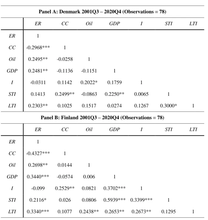
From the correlation tables above, we see that excess returns are significantly negatively correlated to cyclical consumption for all the countries at the 5% level. This could be interpreted as elementary evidence for the countercyclical relationship hypothesised for the two variables. In the 10% significance level, cyclical consumption also possesses negative correlation to the GDP growth variable in all of the countries except Finland. When it comes to excess returns correlation to the other variables, from the tables we see that besides cyclical consumption, GDP growth and long-term interest rates are significantly positively correlated in all the sample countries. Through the entire correlation matrix, for each country, we do not find any values close to one. This gives us confidence that we do not have any multicollinearity issues. Although not presented in this thesis, we perform VIF tests to provide a definitive answer to whether there is a multicollinearity issue. We find that the VIF scores are generally

(30)

below two, with only a few being slightly above two. This implies that we do not have a multicollinearity issue in our data.

Table 3 - Correlation matrices

Panel A: Denmark 2001Q3 – 2020Q4 (Observations = 78)

ER CC Oil GDP I STI LTI

ER 1 CC -0.2968*** 1 Oil 0.2495** -0.0258 1 GDP 0.2481** -0.1136 -0.1151 1 I -0.0311 0.1142 0.2022* 0.1759 1 STI 0.1413 0.2499** -0.0863 0.2250** 0.0065 1 LTI 0.2303** 0.1025 0.1517 0.0274 0.1267 0.3000* 1

Panel B: Finland 2001Q3 – 2020Q4 (Observations = 78)

ER 1 CC -0.4327*** 1 Oil 0.2698** 0.0144 1 GDP 0.3440*** -0.0574 0.006 1 I -0.099 0.2529** 0.0821 0.3702*** 1 STI 0.2116* 0.026 0.0806 0.5939*** 0.3399*** 1 LTI 0.3340*** 0.1077 0.2438** 0.2653** 0.2673** 0.1295 1 (continued)

(31)

(continued)

Panel C: Norway 2004Q4 – 2020Q3 (Observations = 64)

ER 1 CC -0.2633** 1 Oil 0.4263*** -0.1139 1 GDP 0.4846*** -0.2352* 0.1827 1 I -0.0118 0.0622 0.0626 0.2403* 1 STI 0.4555*** 0.0872 0.1208 0.6205*** 0.0562 1 LTI 0.4772*** 0.0241 0.2028 0.4449*** 0.0828 0.3890*** 1

Panel D: Sweden 2007Q1 – 2020Q4 (Observations = 56)

ER 1 CC -0.2793** 1 Oil 0.1929 -0.011 1 GDP 0.2958** -0.2445* -0.166 1 I -0.0213 0.2420* 0.3225** 0.1363 1 STI 0.2528* 0.2267* 0.1166 0.3064** 0.4525*** 1 LTI 0.3447*** 0.004 0.2755** 0.1075 0.1697 0.3918*** 1

*, **, *** denotes significance of 10%, 5% and 1% respectively.

4.3 Regression outcomes

This section outlines the two different regressions for each of the countries included in the sample. First, Panel A in each of the respective tables, shows the regression outcomes from the base model regression as used by Atanasov et al. (2020). We do this in order to see if the cyclical consumption variable has explanatory value on its own. Second, Panel B in each of

(32)

the respective tables, provides the regression outcomes of the extended regression model as outlined in the methodology section. Using these two regressions we compare the coefficients of the cyclical consumption variable to see if the sign or significance of said coefficient changes when the control variables are added into the model. In the next section, we perform two tests (i.e., Likelihood Ratio test and Wald test) to see if the addition of the control variables fits the data better than the base model.

Before we start of the analysis of the outcomes, it is important to note that we do not use the standard t-statistic which is often used in research. In accordance with Atanasov et al. (2020) we employ the Newey-West corrected t-statistic. This alternative test statistics has the benefit that it is robust to possible autocorrelation and heteroskedasticity problems. In order to obtain this statistic, we have to establish a certain number of lags, which we set equal to the value of

h of the particular regression.

Each table presents the coefficient value for the cyclical consumption measure (and additional control variables) for the base regression model (see Atanasov et al. (2020)) and the extended regression model. Both regression models are presented with their accompanying Newey-West corrected t-statistic (in brackets) and its significance level2_{. Additionally, we added the adjusted} R-squared values (with significance levels) for each regression.

Each regression model was performed for five different values of h-quarter ahead excess return as the independent variable. Important to note is the fact that, due to the multiplication effect, excess return values for later values of h are non-stationary. To counter this issue, we decided to take the first difference (i.e., integrated at order 1) of excess returns for the values of h greater than 1. Doing this provides us with stationary dependent variables in each of the regressions. Since the main focus of this paper is h=1, the analysis mainly aims at explaining those coefficients. For the different values of h, the interpretation is very similar and is mainly let to the discretion of the reader.

4.3.1 Results Denmark

Table 4 presents both regressions for Denmark. From the base regression model, we see that the cyclical consumption coefficient significantly (i.e., at various significance levels)

(33)

negatively affects excess returns for all values of h, except for excess returns twelve quarters (i.e., three years in the future). Denmark shows a coefficient of -1.8598, which is significant at 5%. In other words, if cyclical consumption decreases by one percent, the excess returns increase with around 1.86 percent. This implies that, as found by Atanasov et al. (2020), the relationship between cyclical consumption and excess returns is countercyclical. This means that, if consumption is lower compared to its historical values, the marginal utility of consumption increases. Due to this increase in marginal utility of consumption, investors are more inclined to consume instead of investing and therefore require higher stock returns in order to forgo on consumption. Additionally, we find an adjusted R-squared of 0.0761 (i.e., 7.61%) which is significant at 1%. This means that this base model is able to explain around 7.61% of variation in the excess returns. Contrary to Atanasov et al. (2020) we do not find that the explanatory value of cyclical consumption on excess returns for larger values of h increases in size. However, we do find, for most quarters in the future, that cyclical consumption is able to explain excess returns. One possible explanation for this difference with Atanasov et al. (2020) is that we took the first difference of excess returns in order to get stationary time series for those excess returns.

For the full model we see that the cyclical consumption coefficient is still negative and significant in most of the hquarter ahead regressions. At h=1 we see that the coefficient is -1.896272, which is almost identical to the coefficient of the base model. Which seems to imply that the addition of the control variables does not add much value to the explanatory power of cyclical consumption. However, it does provide more evidence to the robustness of this measure, because it is still significant at 5% i.e., it is able to explain excess stock market returns even in the presence of other explanatory variables. For the control variables, we only find that oil prices are consistently able to explain excess returns, for almost every quarter ahead excess returns. We also see that the adjusted R-squared for the full model decreases with the number of quarters ahead, which indicates that the other control variables may not be able to explain excess returns that much in the future. Furthermore, this is clear from the fact that the difference between the adjusted R-squared of the base regression model and full regression model decreases with the number of quarters ahead.

(34)

Table 4 - Regressions Denmark

Panel A: Denmark 2001Q3 – 2020Q4 – Base model

h = 1 h = 4 h = 8 h = 12 h = 16 Coefficient (t-statistic) [Adj. R-sqr.] Coefficient (t-statistic) [Adj. R-sqr.] Coefficient (t-statistic) [Adj. R-sqr.] Coefficient (t-statistic) [Adj. R-sqr.] Coefficient (t-statistic) [Adj. R-sqr.] Cyclical Consumption -1.8598 (-2.05**) [0.0761***] -1.1833 (-1.68*) [0.0338*] -1.52594 (-2.08**) [0.0615**] -1.4318 (-1.57) [0.0586**] -1.7402 (-2.56**) [0.0793**]

Panel B: Denmark 2001Q3 – 2020Q4 – Full model

h = 1 h = 4 h = 8 h = 12 h = 16 Coefficient (t-statistic) Coefficient (t-statistic) Coefficient (t-statistic) Coefficient (t-statistic) Coefficient (t-statistic) Intercept 0.0322878 (1.37) 0.0210029 (1.13) 0.0192166 (0.86) 0.0108601 (0.49) 0.0446713 (1.76) Cyclical Consumption -1.896272 (-2.28**) -0.6628446 (-0.97) -1.489875 (-2.17**) -1.239678 (-1.46) -1.839265 (-3.25**) Oil Prices 0.2029589 (1.9*) 0.1281022 (1.66) 0.2091254 (3.64***) 0.1266219 (1.96*) 0.1473902 (2.16**) GDP growth 2.692241 (1.95*) 1.123943 (1.3) 0.5855288 (0.43) 1.065679 (0.79) -1.366359 (-1.05) Inflation -4.168545 (-1.1) -4.417401 (-1.13) 0.6476036 (0.15) 0.0165554 (0) -2.637617 (-0.84) (continued)

Cyclical consumption and the aggregate stock market: Evidence from the Nordic countries