Political Economy of Infrastructure Investment Allocation : Evidence from a Panel of Large German Cities

FS IV 00 – 03

Political Economy of Infrastructure

Investment Allocation: Evidence from

a Panel of Large German Cities

Achim Kemmerling*

Andreas Stephan**

*

Wissenschaftszentrum Berlin für Sozialforschung

**

Deutsches Institut für Wirtschaftsforschung

February 2000

ISSN Nr. 0722 - 6748

Forschungsschwerpunkt

Marktprozeß und

Unter-nehmensentwicklung

Research Area

Market Processes and

Corporate Development

Achim Kemmerling, Andreas Stephan, Political Economy of Infra-structure Investment Allocation: Evidence from a Panel of Large German Cities, Discussion Paper FS IV 00-03, Wissenschaftszentrum Berlin, 2000.

Wissenschaftszentrum Berlin für Sozialforschung gGmbH, Reichpietschufer 50, 10785 Berlin, Tel. (030) 2 54 91 - 0

Political Economy of Infrastructure Investment Allocation: Evidence from a Panel

of Large German Cities

by Achim Kemmerling and Andreas Stephan

This paper proposes a simultaneous-equation approach to the estimation of the

contri-bution of infrastructure accumulation to private production. A political-economy model

for the allocation of public infrastructure investment grants is formulated. Our empirical

findings, using a panel of large German cities for the years 1980, 1986, and 1988,

sug-gest that cities ruled by a council sharing the State (‘Bundesland’) government's current

political affiliation were particularly successful in attracting infrastructure investment

grants. With regard to the contribution of infrastructure accumulation to growth, we find

that public capital is a significant factor for private production. Moreover, at least for the

sample studied, we find that simultaneity between output and public capital is weak;

thus, feedback effects from output to infrastructure are negligible.

ZUSAMMENFASSUNG

Politische Ökonomie der Allokation von Infrastrukturinvestitionen: Empirische

Evidenz von einem Paneldatensatz großer deutscher Städte

Dieses Papier verwendet ein simultanes Gleichungssystem zur Schätzung des Beitrags

von Infrastrukturinvestitionen zu regionalem Wachstum. Ein polit-ökonomisches

Mo-dell der Allokation von Finanzzuweisungen für öffentliche Investitionen in Infrastruktur

wird formuliert. Unsere empirischen Ergebnisse basierend auf einem Paneldatensatz für

große deutsche Städte in den Jahren 1980, 1986 und 1988 deuten darauf hin, dass

Städ-te, deren Mehrheit im Stadtrat die selbe politische „Couleur“ wie die Landesregierung

hatte, erfolgreicher bei der Zuteilung von Finanzzuweisungen waren. Im Hinblick auf

den Beitrag der Infrastrukturakkumulation auf das Wachstum finden wir, dass

öffentli-ches Kapital ein wichtiger Faktor für die private Produktion ist. Weiterhin, zumindest

für den untersuchten Zeitraum, finden wir, dass die Simultanität zwischen Output und

öffentlichem Kapital gering ist; daher sind Feedback-Effekte von Output zur

Infra-struktur vernachlässigbar.

1. Introduction

This paper examines the role of public capital in private production and provides

a political-economy model of the allocation of public infrastructure investment

grants. From this perspective, our study links the literature on the productivity

effects of infrastructure with the literature on the political-economy of

policy-making.

Since Aschauer published an influential series of papers (1988, 1989a, 1989b,

1989c) about the effects of public infrastructure investment for long-run growth

and productivity in the U. S. and other major countries, there has been an

on-going debate about the role of public infrastructure in generating national

wel-fare. Aschauer (1989a), for example, using a production function approach with

aggregate time-series data for the U. S. from 1949 to 1985, found that the elasticity

of output with respect to a broad measure of public infrastructure was

signifi-cant and of a remarkable magnitude. At a time of widespread concern about the

slowdown of U. S. productivity growth in the 1970’s and 1980’s this finding

sug-gested that the general decline in public infrastructure spending in the U. S. since

the 1970’s could at least partly explain the observed slowdown in productivity

growth.

However, the magnitude of the estimated elasticity of infrastructure capital

in Aschauer (1989a, 1989b, 1995) and other studies (Garcia-Mila and McGuire,

1992; Munnell, 1990a; Munnell, 1990b; Munnell, 1992; Munnell, 1993) is still a

matter of discussion. The main focus of the so-called ‘infrastructure’ debate is

on the interpretation of results and on the appropriate empirical methodology

(Aaron, 1990; Gramlich, 1994; Holtz-Eakin, 1994). For example, it is argued that

the direction of causation is unclear, i.e., whether causality runs from

infrastruc-ture to growth or from growth to infrastrucinfrastruc-ture (Tatom, 1991; Tatom, 1993). In

order to address the problem of causality econometrically several studies have

suggested simultaneous-equation-approaches with public infrastructure

invest-ment as an endogenous variable (e.g., Cadot et al., 1999; Duffy-Deno and Eberts,

1991; de Frutos and Pereira, 1993).

In this paper we adopt the simultaneous equation approach of Cadot et al.

(1999). This not only allows us to address the issue of endogeneity of

infrastruc-ture investments, but also to test whether the German case gives comparable

results to the French ‘pork-barrel politics’ of investment decisions or whether

the peculiarities of the political system in Germany make a different way of

po-litical decisions about the allocation of public infrastructure investments more

plausible.

Previous studies on the role of fiscal federalism for infrastructure policy have

mainly focussed on optimal rules for the provision of infrastructure at different

levels of government (e.g., Hulten and Schwab, 1997). However, it remains an

open question whether infrastructure policies are in reality designed according

to such efficiency considerations. Therefore, the main contribution of our paper

is that we empirically shed light on other potential determinants of infrastructure

policies. What we suppose to be other potential determinants of infrastructure

policy are (i) ‘pork-barrel’ politics due to the influence of firms on the allocation

of investments or (ii) distortions in allocation due to the political affiliation of

governments at different levels. These influences may give rise to results that

might depart substantially from optimal allocation as a result of maximizing

social welfare.

In Cadot et al. (1999) a political-economy model is applied to explain the

regional allocation of public infrastructure investment. Here, we use a similar

model. One difference is, however, that the study by Cadot et al. (1999) focusses

on the allocation of infrastructure investment at the regional level in France,

whereas our study examines the allocation of infrastructure investment grants

at the level of large German cities. Specifically, we derive an econometric model

from a ‘menu auction game’ that was originally developed by Bernheim and

Whinston (1986a, 1986b) and has also been applied by Grossman and Helpman

(1994). This model is based on a very general framework for political-economy

analysis which views economic policy decisions as being a result of the

maxi-mization of objective functions by incumbent politicians under constraints that

are primarily political (see also Dixit, 1996).

Cadot et al. (1999) test their model using a panel data set of French regions and

find a significant relationship between the number of large firms in a region as an

indicator of lobbying strength and the infrastructure investment allocation.

More-over, they also find that political affiliation plays an important role in channelling

public infrastructure towards regions that share the same ‘colour of government’.

The results of Cadot et al. (1999) are perfectly comparable with the political

sci-ence literature referring to the French system of decision-making (Frere, 1998).

High centralization and top-down administration – leaving comparatively little

space for local autonomy – make this system particularly vulnerable to lobbying

by large firms.

In contrast, as a result of federalism the German decision making system is

deeply nested and intertwined. The spheres of competence and control as well as

the financing of investment are not as separated as it is in the case of France or

the U. S. but they are overlapping and mutually dependent (Scharpf, 1988). This

makes an extension of the basic model inevitable.

Investment in municipal infrastructure usually consists of two parts:

auto-nomous investment and investment grants. Whereas the former is a matter of

decision for municipal councils the latter is predominantly provided by the

fed-eral States (‘Bundesl¨ander’). Because of the increasing role of investment grants

since the 1970’s we assume that these financial resources are heavily contested

among manufacturing firms. With fiscal federalism diluting political

accountabil-ity and channels of interest management, these firms might find it difficult to

divert infrastructure investment to their regions. This is a result of what we call

the logic of ’intertwined politics’. A possible exception might exist if local council

members could short-cut the bargaining process by means of vertical political

alignments.

With our empirical model we can test these two ideas – pork-barrel vs.

in-tertwined politics – on a panel data set consisting of 91 German cities for the

years 1980, 1986 and 1988. As in Cadot et al. (1999) we use a

simultaneous-equa-tions approach to estimate the relasimultaneous-equa-tionship between infrastructure investments,

output, policy and lobbying variables. One of our main findings is that political

affiliation, measured by the coincidence of party colour between state and local

government, is decisive in explaining the distribution of investment grants.

The remainder of this paper is organized as follows: In section 2, we discuss the

political lobbying framework, which Cadot et al. (1999) applied to the regional

allocation of infrastructure investments in France. In this section, we also deal

explicitly with two peculiarities of the German case in comparison to France:

investment grant policy and fiscal federalism. Section 3 motivates our model of

the allocation of infrastructure investment grants across cities. In section 4 we

de-scribe the panel data used in the analysis and present the results of our empirical

estimations. Section 5 provides conclusions.

2. Modelling endogenous infrastructure investment decisions in Germany

2.1. THE ORIGINAL FRAMEWORK OF POLITICAL LOBBYING FOR

In Cadot et al. (1999) a political-economy model is applied to explain the regional

allocation of public infrastructure investment. This model is based on a general

framework for political-economy analysis that views economic policy decisions

as a result of the maximization of objective functions by incumbent politicians

under constraints that are primarily political.

The starting point of this framework is the assumption that firms offer

cam-paign contributions to incumbent politicians in return for additional spending.

These contributions reflect the firms’ marginal willingness to pay for additional

infrastructure. Therefore, they reflect infrastructure’s marginal contribution to

firm value, both on the supply side, through the infrastructure’s contribution to

productivity in all sectors, and on the demand side for the construction industry

itself.

In the context of infrastructure investment the motivation for lobbying is the

following: Firms have vested interests in the quality of the infrastructure in those

municipalities where they have high sunk investment, which is usually the

loca-tion of producloca-tion. The authors argue that large firms will lobby harder because

these firms produce, on average, for more distant markets and therefore use

pub-lic infrastructure more intensively than others. Moreover, large firms have two

strategic advantages. They are able to overcome problems of collective action

more easily than small enterprises and their form of lobbying – personal contacts

between big business and high politics – may be more efficient than the lobbying

activities of small firms.

The underlying model of the political decision making system is quite simple:

Local politicians act as contribution collectors, providing their affiliated parties’

headquarters with locally generated campaign contributions. Furthermore,

lo-cal politicians propose public infrastructure projects – on behalf of the voters –

that are approved by central government. In contrast to Grossman and Helpman

(1994), Cadot et al. (1999) thus allow for two different levels in the decision

mak-ing process of infrastructure policy. Pointmak-ing to the high level of centralization the

authors argue that the basic model holds for the French case. Therefore, there is

no principal agent problem between local and central policy makers.

However, the assumption of a simple representative democracy, where all

de-cisions are made at the highest government level and than implemented by

obe-dient lower administrative officials is not valid for the German federal system as a

broad array of studies show (Garlichs, 1986; Scharpf, 1988; Scharpf, 1999).

There-fore, we will have to look with greater accuracy at the way German infrastructure

investment is financed.

2.2. THE SIGNIFICANCE OF

GERMAN INVESTMENT GRANT POLICY

Infrastructure investment projects in Germany are usually financed from the

re-sources of two or more levels of governments. Here, we consider two different

financial sources for infrastructure investment: autonomous investment by

mu-nicipalities and investment grants

_{provided by other institutions, e.g. the central}

government (‘Bund’), the federal States (‘Bundesl¨ander’) the European

Recov-ery Program (ERP) or horizontal fiscal exchange mechanisms. In our context the

‘Bundesl¨ander’ are of particular interest because they provide the major part of

these grants (Pohlan, 1997). The procedure for starting a new infrastructure

in-vestment project is a complex arrangement between the local government, which

makes a proposal in the first stage of project planning, and the ‘L¨ander’ or ‘Bund’

administration that grants an investment subsidy. Because of the growing fiscal

tension in the local budgets (Pohlan, 1997), the role of investment subsidies has

risen through the 1980’s. In 1980 the ratio between investment subsidies from

‘Bund’, ‘Bundesl¨ander’ and the ERP to total investment in road infrastructure

was about 24 percent, whereas in 1988 this ratio rose to 46 percent. The

munici-palities’ dependency on investment grants also makes it difficult for them to plan

investment projects autonomously. One reason for this is the overall increase of

insecurity in the planning process, as local decision makers cannot anticipate the

correct amount of future transfer payments (Bundesamt, 1986: 913).

Second, mixed financing of infrastructure projects undermines local political

autonomy. An example may illustrate this point: Schmals (1982) cites a case study

about public transportation in Munich at the end of the 1970’s. Two alternative

plans to improve public transport existed. The first plan proposed the

construc-tion of a network of underground railways to alleviate inner-city traffic. The

majority of city council members favoured this project. The second proposal, the

construction and improvement of a municipal railway system, was backed by the

Bavarian government. Because the Bavarian ‘Bundesland’ linked an investment

grant to the realization of the second project, the city council had to give in. Thus,

in this case investment grant prospects had a decisive impact on the bargaining

power between the two governmental levels.

The amount of investment subsidies granted to local infrastructure projects

formally depends on such external factors as car density, length of the road

net-work, etc. But as Garlichs (1986) shows in the case of infrastructure funds for

highways, the actual amount of money is a matter of intense bargaining between

lower level governments and the higher level. As for highways, the authorities

involved are the ‘Bund’ and the ‘Bundesl¨ander’ governments. But this also

ap-plies in the case of local infrastructure projects (Garlichs, 1986: 136). Frequently,

the result of the bargaining process is a quota system that reflects the traditional

or even legally settled principle of unanimity.

The increasing importance of investment grants for the realization of

invest-ment projects led us to model both sources (grants and autonomous investinvest-ment)

separately in our simultaneous equation approach (see section 3 below). In order

to describe this simultaneous determination properly, our model has two

equa-tions: one which describes the autonomous investment decisions of the cities and

one which describes the level of investment grants the cities receive from higher

level governments. Furthermore, autonomous investment enters the grants

equa-tion and vice versa.

From this model it is also possible to answer the question of whether the

re-lationship of autonomous investments and investment grants is complementary,

substitutional or neutral. But the existence of two mutually dependent levels of

government that both intervene in the decision making process of infrastructure

policy has even broader implications for the lobbying framework.

2.3. INFRASTRUCTURE POLICY AND THE

‘LOGIC OF INTERTWINED POLITICS’

GERMANY

The underlying assumption of a simple (Westminster) representative democracy

seems to be severely violated in the German case. One of the reasons for this is the

peculiar nature of German federalism which has been characterized in literature

as a ‘unitary federal state’ (‘Verbundf ¨oderalismus’ or ‘f ¨oderativer Bundesstaat’).

In Germany, spheres of competence and control, as well as the financing of

investment, are not as separated as for example in the case of U. S. federalism.

Rather it is overlapping and mutually dependent. Therefore, although the states

(’Bundesl¨ander’) and the municipalities (‘Kommunen’) are exclusively

respon-sible for the main part of public infrastructure in a formal sense, investment

decisions also depend on the amount of public subsidies which come from either

the federal state, the federal states or from the European Union.

Moreover, German federalism is constitutionally obliged to balance local

au-tonomy and the uniformity of living conditions throughout German territory.

Humplick and Moini-Araghi (1996) show that this often results in a less efficient

provision of public infrastructure. Germany has a high standard of road

infras-tructure but its construction costs are higher than in other OECD countries. As

Humplick and Moini-Araghi (1996: 32) put it ‘the equity objective overrides the

efficiency objective’. These obligations in German federalism create the need for

a network of horizontal and vertical bargaining institutions that coordinate the

interests of the several governmental levels.

In our case it is difficult to specify the exact locus of decision making power for

road infrastructure investment. Abstracting from the federal state or relationships

with the E. U. , we have two important levels in the German political system, each

with its own interests: ‘Bundesl¨ander’ and local governments. ‘Bundesl¨ander’

governments want – among other things – to maximize the welfare of their

terri-tory and try to balance diverging regional developments. The local governments

try to get as many investment grants as possible (pork-barrel politics). Both levels

are forced to bargain as the ‘Bundesl¨ander’ government wants to intervene but

lacks information about where to do so whereas the local governments compete

with each other for scarce resources.

This phenomenon is easily visible in all policy areas that bind different

Ger-man government levels together, and it is often cited as ‘intertwined politics’

(‘Politikverflechtung’). In our context it describes the pathological situation when

municipalities and the States lack the autonomy to make their own decisions,

whereas the ‘Bundesland’ simultaneously lacks information to control the other

governmental levels, so that neither of the two governmental levels is able (and

inclined) to provide investment allocation efficiently. Moreover, political

account-ability is diluted because there is no single agent that bears all the

responsibil-ity for a single policy. There are many studies that show the negative effects of

‘intertwined politics’ in Germany (Scharpf et al., 1976; Scharpf, 1988; Scharpf,

1999)

This might produce perilous effects for pluralistic lobbying such as in U. S.

interest mediation: a complex and closed system of decision making could be a

serious problem even for powerful lobbies.

In other words, large firms will find

it extremely difficult to divert infrastructure investments to their region if there

is no way of short-cutting the bargaining process by means of vertical political

alignments.

In our political-economy framework we are especially interested in political

variables that influence the allocation of investment subsidies. We argue that

because of the complex federal system as described above by the notion of

‘in-tertwined politics’ those local governments whose political ‘colour’ corresponds

to that of the ‘L¨ander’-government get more investment subsidies, because this

lowers the transaction costs of information transmission between governments.

The identity of political colour shortcuts this bargaining process and favours

certain municipalities by means of party loyalty.

Whether German infrastructure policy follows the logic of the lobbying

frame-work, that of ‘intertwined politics’ or both is the fundamental question for the

empirical estimation. But let us first summarize the structure of our model with

the whole set of hypotheses.

3. Structure of the model

Our model is based on 3 equations, which we label as (i) production function, (ii)

city i

s lobbying function and (iii) city i

s infrastructure investment function.

3.1. PRODUCTION FUNCTION

To begin with, we assume that the production Q

of the manufacturing sector can

be described as

Q

=

f

(

t, K

, L

, G

)

,

i

=

1 . . . N,

t

=

1 . . . T,

(1)

where t denotes time, Q

output, K

private capital, L

labour input and G

de-notes the infrastructure stock in city i. In addition, city i’s infrastructure stock G

is defined as

G

= (

1

− γ)

G

+

INV

+

GRANTS

,

(2)

where

γ

denotes the depreciation rate of public capital, INV

denotes

infrastruc-ture investment, and GRANT

denotes infrastructure investment grants given to

city i from the State (‘Bundesland’) government. Therefore, total infrastructure

investment in city i is defined as INV

+

GRANT

.

Assuming a Cobb-Douglas functional form for the manufacturing sector’s

pro-duction function in city i at time t we get

Q

=

A0

exp

(α

t

)

L

K

G

,

(3)

where

α

denotes the elasticity of output Q with respect to input X, and X

∈

{

t, L, K, G

}

. Dividing by L

, (3) becomes

q

=

A0

exp

(α

t

)

k

g

L

˜ αL

it

,

(4)

where small capitals denote variables in terms of the labour input L and ˜

α

is

Note that ˜

α

will equal zero if returns to scale are constant with respect to all

inputs, i.e., L, K and G; and ˜

α

−α

will equal zero if returns to scale are constant

with respect to private inputs L and K.

3.2. CITY

i

City i

s lobbying function for state investment grants can be described as follows

GRANT

=

f

(

Q

, INV

, policy variables, lobbying variables

)

.

(5)

Thus, we assume that GRANT

depends on investment decisions, i.e., INV

, but

also on a set of policy, ‘lobbying’ and other (exogenous) variables. For instance, we

expect that a city will receive more grants if it has a lower initial income, or a

lower growth of Q

in a previous period relative to other cities. Subsequently, the

‘Bundesland’ government will use its investment grant policy to promote growth

in ‘poorer’ cities. On the other hand, we assume that firms in the manufacturing

sector have sunk investment giving them vested interests in the quality of

in-frastructure in cities where they have establishments and production units. The

reason is that firms of the manufacturing sector quite often produce for more

distant markets than for example firms of the service sector. Therefore, firms in

the manufacturing sector in a given city should be expected to lobby harder than

other firms for the maintenance and upgrading of that city’s infrastructure.

The form of lobbying we suppose is fairly simple. Firms offer campaign

contri-bution to local politicians in return for additional infrastructure spending. Local

politicians act as campaign contribution collectors, final decisions about

infras-tructure investment grants are made at the state (‘Bundesland’) level.

The lobbying game can be motivated as follows. Following Bernheim and

Whinston (1986a), and Grossman and Helpman (1994), lobbying activities are

modelled as a ‘menu’ auction, whereby several lobbies bid non-cooperatively

for influence over a policy variable determined by an auctioneer, in our case the

‘Bundesland’ government. The main difference between a menu and a standard

auction is, that in the former bids are functions and not just a non-negative real

number as in the standard auction and all players end up paying something,

whereas in the standard auction only the winner pays.

To formalize this idea, let us assume that there is a set L of principals (lobbies),

in our case the councils of large cities. The auctioneer, in our case the ‘Bundesland’

government, may choose an allocation of public investment grant allocations

grant

= (

grant1t

, ..., grant

)

from a set

X. The set X is bounded so that each

investment grant policy grant

must lie between some minimum grant

i

and some

maximum grant

.

In each period, cities indexed by i

=

1, ..., n simultaneously face the

‘Bundes-land’ government, if it is of the same political affiliation, with monetary

trans-fer oftrans-fers C

(

grant

)

conditioned on the vector grant

. These monetary transfers

can be interpreted in our context as campaign contribution from

manufactur-ing firms which have establishments in a given city. Hence, local politicians act

as contribution collectors. The ‘Bundesland’ government then chooses a value

grant

of the policy vector grant

that maximizes an objective function

G[

grant

,

∑

C

(grant

)]

. Finally, the cities make transfers C

(grant

)

to the ‘Bundesland’

government as promised.

An equilibrium of this game is a set of contribution functions

{

C

(

grant

)}

,

one for each city, such that each one maximizes the welfare of the city given the

schedules set by the other cities and the anticipated political optimization by the

‘Bundesland’ government, and a vector grant

that maximizes the government’s

objective taking the contribution schedules as given (Grossman and Helpman,

1994).

Social welfare will be of concern to the government because voters are more

likely to re-elect a government that has established a high standard of

liv-ing. Suppose the ‘Bundesland’ governments objective function is given as

G =

∑

C

(

grant

) +

aW

(

grant

)

with weight a

≥

0, and W represents aggregate

gross-of-contributions welfare. Thus, the government objective function is given

as a weighted sum of campaign contributions and aggregate welfare.

Aggre-gate gross welfare is defined as W

≡

_∑

w

(grant)

, where w

is the level of

welfare

_{in city i, and w}

i

depends on the level of grants with

∂w

/

∂grant

>

0,

∂

_w

i

/

∂grant

<

0. The equilibrium of this game can be characterized as follows.

LEMMA 1. (B-W, 1986; G-H, 1994)

({

C

}

, grant

)

is a subgame-perfect Nash

(a) C

∈

C

for all i

∈

L,

(b) grant

maximizes

∑

C

(grant) +

aW

(grant

)

on

X,

(c) grant

maximizes W

(

grant

) −

C

(

grant

) +

∑

C

(

grant

) +

aW

(

grant

)

for

ev-ery j

∈

L,

(d) for every j

∈

L there exists a grant

∈

X that maximizes ∑

C

(

grant

) +

aW

(grant

)

such that C

(grant

) =

0.

For a proof of this Lemma see Bernheim and Whinston (1986a), Lemma 2.

Con-dition (a) states that the chosen contribution schedule is among those that are

feasible. Condition (b) states, that given the contribution schedules offered by the

cities, the government sets its policy to maximize its own welfare. Condition (c)

stipulates that for every city i, the equilibrium grant vector must maximize the

joint welfare of that city and of the government, given the contribution schedules

of the other lobbies. Condition (d) states that there is always an optimal action for

each city with zero contribution which the government finds equally attractive as

the equilibrium policy vector grant

.

One appealing characteristic of this game, which is of special relevance for

our problem of grant allocation, is that in equilibrium players announce their

true willingness-to-pay. Thus, a truthful payment function for lobby i rewards the

government for every change in the action with exactly the amount of change in

the lobbies’ welfare. This resembles the so-called Groves-Clarke mechanism in

the context of bidding for public projects (Clarke, 1971; Groves, 1973).

From this model, we expect that (i) the political affiliation of a city’s council,

and (ii) the number of manufacturing firms in a given city will affect the level of

grants which a city receives.

3.3. CITY

i

Finally, we assume that public investment in city i can be described by the

equa-tion

INV

=

f

(

Q

, GRANT

, policy variables, exogenous factors

)

.

(6)

Thus, city i

s investment (net of state grants) depend on investment grants but

also on a set of policy variables. For instance, if the expected productivity effects

of infrastructure in a city are high, the level of investment in this city should

be higher compared to cities where expected productivity effects are lower.

Fur-thermore, we expect that the higher the trade tax income of a city is, the more

infrastructure projects it is able to finance. Similarly, the lower the level of debt

that a city has, the more infrastructure projects the city is able to carry out. Finally,

we expect that the higher the number of cars in a city, the higher will be the

demand for additional road infrastructure projects.

Table I. Variable description and cities

Variable Description

Q Value added, manufacturing sector, million 1980 DM L Hours worked in manufacturing sector, million hours

K Capital stock in manufacturing, million 1980 DM (from Deitmar, 1993 G Public infrastructure stock, million 1980 DM, (from Seitz, 1995) INV Infrastructure investment, million 1980 DM

GRANT Infrastructure investment grants, million 1980 DM DEBT Total debt of city, million 1980 DM

TAX Trade tax (‘Gewerbesteuer’) income of cityi,million 1980 DM CARS Number of registered cars per capita

NFIRMS Number of manufacturing firms in cityi

DMIN ING Dummy variable equal to1when mining industry is present in cityi

PARTISAN Percentage of members in city council with the same political affiliation as the government of ‘Bundesland’

4. Empirical implementation

4.1. DATA

We use a panel data set consisting of 91 German cities and three distinct years.

Table 1 provides a brief overview of the variables used in the analysis.

The data is taken from the ‘Statistical Yearbook of German Cities and

Muni-cipalities’,

_{which contains information about 500 German municipalities and}

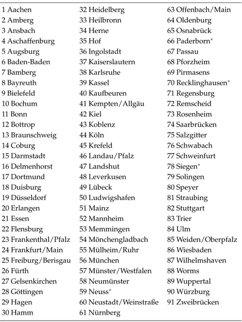
Table II. Cities in panel

Cities in Panel

1 Aachen 32 Heidelberg 63 Offenbach/Main 2 Amberg 33 Heilbronn 64 Oldenburg

3 Ansbach 34 Herne 65 Osnabr ¨uck

4 Aschaffenburg 35 Hof 66 Paderborn∗ 5 Augsburg 36 Ingolstadt 67 Passau 6 Baden-Baden 37 Kaiserslautern 68 Pforzheim 7 Bamberg 38 Karlsruhe 69 Pirmasens 8 Bayreuth 39 Kassel 70 Recklinghausen∗ 9 Bielefeld 40 Kaufbeuren 71 Regensburg 10 Bochum 41 Kempten/Allg¨au 72 Remscheid

11 Bonn 42 Kiel 73 Rosenheim

12 Bottrop 43 Koblenz 74 Saarbr ¨ucken 13 Braunschweig 44 K ¨oln 75 Salzgitter

14 Coburg 45 Krefeld 76 Schwabach

15 Darmstadt 46 Landau/Pfalz 77 Schweinfurt 16 Delmenhorst 47 Landshut 78 Siegen∗ 17 Dortmund 48 Leverkusen 79 Solingen 18 Duisburg 49 L ¨ubeck 80 Speyer 19 D ¨usseldorf 50 Ludwigshafen 81 Straubing 20 Erlangen 51 Mainz 82 Stuttgart

21 Essen 52 Mannheim 83 Trier

22 Flensburg 53 Memmingen 84 Ulm

23 Frankenthal/Pfalz 54 M ¨onchengladbach 85 Weiden/Oberpfalz 24 Frankfurt/Main 55 M ¨ulheim/Ruhr 86 Wiesbaden

25 Freiburg/Berisgau 56 M ¨unchen 87 Wilhelmshaven 26 F ¨urth 57 M ¨unster/Westfalen 88 Worms

27 Gelsenkirchen 58 Neum ¨unster 89 Wuppertal 28 G ¨ottingen 59 Neuss∗ 90 W ¨urzburg 29 Hagen 60 Neustadt/Weinstraße 91 Zweibr ¨ucken 30 Hamm 61 N ¨urnberg

∗_{not included because of missing values for one or more variables}

cities. For reasons of comparability we have selected 91 cities that are

predom-inantly self-administered at the local level (‘kreisfreie St¨adte’). This is of special

importance as part of our model explicitly deals with the political-economy of

these administratively comparable cities. Table 2 displays the names of the cities

in the sample. Note that some cities have been excluded from the estimation due

to missing values for one or more variables.

Table III. Summary statistics

Variable Mean Std.Dev. C.V. Minimum Maximum

Q 2099.1 2500.3 119.1 144.3 15718.8 G 2468.8 2834.5 114.8 302.5 18176.1 K 4087.7 5007.6 122.5 252.0 25714.9 L 30.74 29.08 94.6 2.4 168.2 INV 93.6 123.8 132.3 8.1 1040.4 GRANT 32.8 44.7 136.3 0.8 266.1 DEBT 407.9 509.1 124.8 14.3 3066.7 TAX 135.6 210.4 155.2 7.1 1314.6 CARS 0.459 0.054 11.9 0.347 0.613 NFIRMS 124.0 101.1 81.5 21 637 DMIN ING 0.126 0.333 263.4 0 1 PARTISAN 45.9 8.0 17.5 29.0 68.2

Total number of observations with non-missing values: 261

Output (Q), measured as gross value added of a city’s manufacturing sector,

is taken from a joint publication of several German statistical offices.

_{These data}

are not available for each year, so we could use only the three years 1980, 1986,

and 1988 for our analysis.

The private capital stock (K) of the manufacturing sector is taken from Deitmar

(1993). It is given in 1980 prices and has been also carefully corrected for the

terri-torial reforms that occurred in the 1970’s in Germany.

_{The infrastructure capital}

stock (G), which includes investment both for construction and equipments, is

taken from Seitz (1994) and is also measured in 1980 prices.

Annual investment in infrastructure (INV) has been obtained from the

statisti-cal yearbook mentioned above. From the same source we have also obtained the

following variables: labour input (L), operationalized by the number of working

hours in the manufacturing sector; special grant-in-aids (‘Finanzzuweisungen’)

for investments (GRANTS) from ‘Bundesl¨ander’, ‘Bund’ or ERP; several

mea-sures of the financial situation of a city like the cumulated debt (DEBT) or trade

taxes (TAX) which are levied at the local level of cities, the number of four wheel

vehicles per 1000 inhabitants (CARS), and the number of manufacturing firms

(NFIRMS) in a city.

Furthermore, we constructed a political variable denoted as PART ISAN to

measure the congruence between the local city government and the ‘Bundesland’

government. It gives the percentage of seats in the city council with the same

po-litical affiliation as the ‘Bundesland’ government where the city is located. Thus,

this variable is an indicator of the political ‘lobbying’ strength of a city relative to

the other cities in the same ‘Bundesland’.

Table 3 displays some descriptive statistics of the variables. Note, for instance

that grants are on average about one-third of autonomous investments. Annual

infrastructure investment undertaken by cities is on average about 3.8 percent of

the existing infrastructure capital stock. The mining industry is present in about

13 percent of cities in our sample. The partisan variable is on average 45.9 percent,

with a minimum of 29.0 and a maximum of 68.2 percent.

As described in the previous section, our model contains the following 3

equa-tions:

Production function

ln q

= α

+ α

+ α

ln k

+ α

ln

(

g

+

inv

+

grant

) +

α

˜

ln

(

L

)

+α

DMIN ING

+ ν

,

(7)

Lobbying function

grant

= γ

+ γ

+ γ

inv

+ γ

bq

+ γ

q

+ γ

g

+γ

NFIRMS

+ γ

PART ISAN

+γ

DMIN ING

+ ν

,

(8)

Investment function

inv

= β

+ β

+ β

grant

+ β

bq

+ β

q

+β

g

+ β

α

q

/

g

+ β

debt

+β

tax

+ β

CARS

+ β

DMIN ING

+ ν

,

(9)

where we assume that

ν

, k

=

1, 2, 3, are i.i.d. variables with mean zero and

variance

σ

. Note, that variables with names in lower case are divided by the

We include a dummy variable DMIN ING to all equations indicating whether

or not the mining industry is present in city i. Equation (7) refers to the production

function of the manufacturing sector in city i at time t. Equation (8) describes the

infrastructure investment grants which city i receives, whereas equation (9) refers

to the autonomous infrastructure investments undertaken by city i.

From the Cobb-Douglas production function, marginal productivity of

infras-tructure capital is defined as

∂Q

/

∂G

= α

Q

/

G

. We included this measure of

the expected productivity effects of infrastructure both in the ‘lobbying’ and the

‘investment’ function. Since g

also contains current investment inv

, we replaced

it with its lagged value g

.

Our estimation strategy is as follows: first, we estimate a ‘Between’ regression.

Thus, for each city observations for the years 1980, 1986 and 1988 are averaged.

Then, we estimate a two-way fixed-effects (‘Within’) Panel data model, where

dummy variables for cities and years are included. Finally, a restricted version

of the previous model is estimated, where instead of the whole set of 81 city

dummy variables only a set of 8 ‘Bundesland’ dummy variables is included. The

usual rank and order conditions for the identification of the parameters in the

simultaneous system of equations are satisfied.

Table IV shows the results of the ‘Between’ regression. The estimates of the

‘Be-tween’ regression can be interpreted as ‘long-run’ parameters. Furthermore, the

‘Between’ analysis is appealing in our context since we are interested in the

allo-cation across cities, and this cross-sectional variation is captured by the ‘Between’

variance.

The number of observations for this model is 87. In order to compare the

results for different estimators, the simultaneous system (7)-(9) was estimated

with (1) non-linear OLS, (2) non-linear 2SLS, (3) non-linear 3SLS, and (4) with

non-linear Full-Information Maximum Likelihood (FIML). Dummy variables for

‘Bundesl¨ander’ (denoted ‘BuLa’) have been also included.

It is worth noting that for all 3 equations the fit of regression is remarkably

good. We performed White’s (1980) test for heteroscedasticity, which because of

its generality is also a test for misspecification of the model. None of the tests

is significant at a 10 percent level, thus the null hypothesis of homoscedasticity

is not rejected. The condition numbers are between 82 und 94. Except for the

Table IV. Empirical results for ‘Between’ regression

Nonlinear OLS 2SLS 3SLS FIML

Production function: ln qit

αi BuLa-effects∗∗ BuLa-effects∗∗ BuLa-effects∗∗ BuLa-effects∗∗∗ αK 0.668 (7.78) 0.691 (7.93) 0.685 (7.87) 0.658 (8.26) αG 0.130 (1.70) 0.082 (1.00) 0.086 (1.04) 0.130 (1.82) ˜ αL 0.033 (0.79) 0.020 (0.47) 0.023 (0.55) 0.039 (1.02) α_MINING -0.474 (-4.61) -0.484 (-4.68) -0.483 (-4.68) -0.474 (-4.94) Whiteχ2_{(39) 19.0 18.42 18.52 19.17} R2 _{0.667 0.665 0.665 0.667}

Lobbying function: grantit

γi BuLa-effects∗ BuLa-effects BuLa-effects BuLa-effects∗ γinv 0.162 (2.44) 0.118 (0.68) 0.111 (0.64) 0.157 (1.01) γbq -0.733 (-2.78) -0.799 (-2.62) -0.809 (-2.66) -0.729 (-3.27) γq80 -0.006 (-2.28) -0.008 (-2.06) -0.008 (-2.14) -0.006 (-3.17) γG 0.011 (4.55) 0.013 (2.68) 0.013 (2.75) 0.011 (2.54) γ_PROD 1.616 (0.97) 3.919 (0.74) 3.891 (0.78) 1.586 (1.15) γ_PARTISAN 0.025 (3.18) 0.026 (3.04) 0.026 (3.03) 0.025 (3.57) γ_NFIRMS 0.001 (0.52) 0.001 (0.48) 0.001 (0.62) 0.001 (0.56) γ_DMINING 0.289 (1.39) 0.256 (1.03) 0.253 (1.02) 0.285 (1.26) Whiteχ2_{(85) 86.82 86.78 86.77 86.82} R2 _{0.756 0.753 0.753 0.756}

Investment function: invit

βi BuLa-effects∗∗∗ BuLa-effects∗∗ BuLa-effects∗∗ BuLa-effects∗∗∗

βgrant 0.373 (2.09) -0.221 (-0.40) -0.173 (-0.31) 0.029 (0.06) βbq 0.210 (0.46) 0.056 (0.10) 0.034 (0.06) -0.023 (-0.05) βq80 -0.001 (-0.23) -0.001 (-0.14) -0.003 (-0.39) -0.005 (-1.21) βG 0.028 (6.47) 0.034 (4.16) 0.034 (4.19) 0.033 (4.37) β_PROD -1.170 (-0.51) -4.507 (-0.62) -3.698 (-0.57) -1.324 (-0.68) β_DEBT -0.055 (-3.26) -0.057 (-3.07) -0.057 (-3.08) -0.056 (-3.62) β_TAX 0.013 (0.60) 0.015 (0.63) 0.011 (0.48) 0.015 (0.77) β_CAR 3.032 (1.02) 4.092 (1.23) 4.112 (1.26) 3.544 (1.28) β_DMINING -1.022 (-3.11) -0.764 (-1.78) -0.811 (-1.9) -0.926 (-2.51) Whiteχ2_{(86) 87.0 87.0 87.0 87.0} R2 _{0.834 0.806 0.810 0.823} Condition-Number 82.36 88.34 94.05 89.53 Obs. 87 87 87 87

t-values are given in parentheses. ∗at 10 %,∗∗at 5 %,∗∗∗at 1 % significant. Hausman test statistic 2SLS vs. OLS: 1.484 (χ2_{), 45 df.}

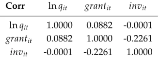
Table V. Correlation of equation resid-uals from OLS estimation, table IV

Corr ln qit grantit invit

ln qit 1.0000 0.0882 -0.0001

grantit 0.0882 1.0000 -0.2261

invit -0.0001 -0.2261 1.0000

parameters of endogenous variables (

α

,

γ

,

γ

,

β

,

β

),

parame-ter estimates turn out to be fairly robust with respect to the applied estimation

methodologies (OLS, 2SLS, 3SLS, FIML). The correlations of equation residuals

from OLS estimation are presented in table V. These correlations are relatively

low, indicating that there will not be much gain in efficiency from the system

estimation methods 3SLS and FIML compared to OLS.

We also performed a Hausman test on the difference of estimates between OLS

and 2SLS estimation. This test statistic is 1.484 with 45 degrees of freedom, which

implies that estimates of OLS and 2SLS do not differ significantly. Hence, due to

lower variance of OLS compared to instrumental variable techniques the former

is the preferred estimation method.

The estimate for private capital is significant at a 1 percent level for all

estima-tions. In contrast to this, the estimate for infrastructure capital is only significant

at a 10 percent level for OLS and FIML estimation. Constant returns to scale are

not rejected for all estimations, which can be concluded from the insignificance

of ˜

α

. The dummy variable DMIN ING, indicating whether the mining industry

is present in city or not, is highly significant with a negative coefficient. Thus,

expected output of the manufacturing sector in cities with mining is lower than

in cities without a mining industry. The ‘Bundesl¨ander’ dummy variables are

significant. Hence, expected output of cities’ manufacturing sectors are different

depending on the ‘Bundesland’ in which they are located.

Turning to the lobbying function, we find for OLS estimation that the level of

(autonomous) investment

γ

is positively related to the level of grants which

city i receives. Thus, grants and investment appear to be complementary to each

other, i.e., there is no indication of a substitution effect of grants on investment.

Furthermore, we find that the lower a city’s initial income q

and the lower

its growth rate

bq of the manufacturing sector in the period 1980-88, the higher

is the expected level of grants a city receives. Hence, policy considerations of

higher level governments to promote growth in ‘poorer’ cities or cities with poor

economic performance seem to be evident.

On the other hand, expected productivity effects (

γ

) of infrastructure

investment appear not to matter for the allocation of investment grants. One

explanation for this finding is given by Seidel and Vesper (1999). They state that

investment grant decisions from the federal government are based on consensus

between all states, so that ‘[...] this approach is prone to produce decisions that

carefully skirt all areas of conflict. In terms of economic efficiency, the solution

will often seem less than optimal, as there can be no guarantee that the money is

being put to its most productive use.’

Furthermore, the higher the infrastructure stock of the city (

γ

), the higher

the expected level of grants it receives. Since the ‘L¨ander’ dummy variables are

significant at a 10 percent level, there is some evidence that there is a systematic

difference between the level of grants cities in the various ‘Bundesl¨ander’ receive.

Lobbying activities of manufacturing firms, as indicated by the coefficient for

the number of firms (NFIRMS

)

, do not appear to be important for

infrastruc-ture investment grant decisions. However, the estimate for the partisan variable

(PART ISAN) is significant, which means that the expected level of grants is

higher if the local city council and the state (‘Bundesland’) government share

the same political affiliation. We interpret this finding as an indication that

short-cutting of the bargaining process between cities and the federal states

govern-ments by means of vertical political aligngovern-ments is indeed important.

Turning to the investment function, from the significance and the positive sign

of

β

in the OLS estimation we conclude, again, that grants and investments

are complementary. In contrast to the lobbying function, policy variables, such

as the initial income q

or the growth rate

bq, are not significant predictors for

expected investment level of city i. Also, the expected return from infrastructure

investments,

β

, is not significant. However, we find that the higher the level

of DEBT, the lower the city’s infrastructure spending, which is a very plausible

finding. This corroborates our initial assumption that the financial room for

ma-noeuvre is decisive for local infrastructure investments. On the other hand, trade

tax income of a city

β

is not significant for its investment decisions. Expected

investments are lower in cities where the mining industry is present. Finally,

the coefficient for the number of cars (

β

) is not a significant determinant for

investment decisions.

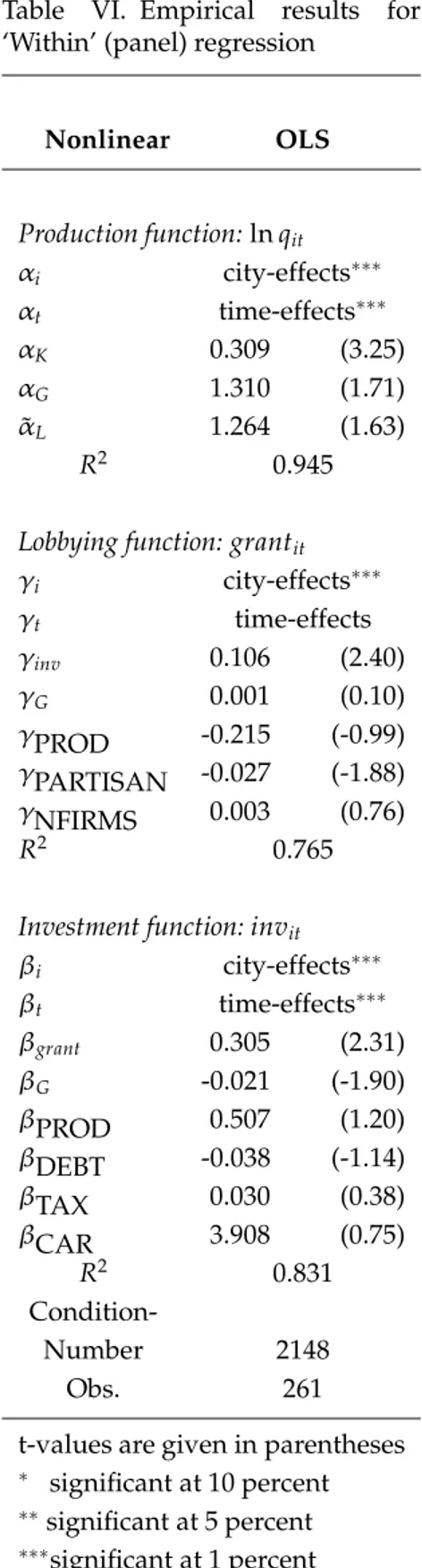
Table VI presents the results for the ‘Within’ (fixed-effects) regression. This

regression is based on the full sample of 261 observations having non-missing

values. Here we have included dummies both for cities as well as for time

peri-ods. Note first that for this model it is not possible to include the variables q

,

bq

and DMIN ING

because these are constant for each city i and hence would be

perfect collinear with the fixed-effects for cities if included.

It turns out that the city effects are highly significant for all equations, whereas

the time-effects are only significant for the production and investment function.

The fit of the production function is fairly high (R

_{is about 0.95) but the}

esti-mated coefficients are not plausible, except that for private capital (

α

). The high

condition number of 2148 indicates that for this model the degree of collinearity

might cause estimation problems. This is due to the high correlation of the fixed

effects with some of the variables (see also Ai and Cassou, 1997). This is

partic-ularly true for variables which do not vary much (i.e. have not enough ‘Within’

variation) over the 3 sample years 1980, 1986, and 1988, e.g. the infrastructure

stock G. In fact, the estimation of the parameter

α

is adversely affected by this

multicollinearity.

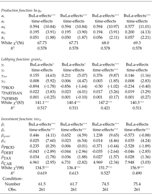
A preferred estimation strategy is therefore to impose some restrictions on the

parameters in order to reduce the degree of collinearity. Table VII gives the results

for a restricted regression. It is again based on 261 observations as in table VI.

However, in table VII we have included ‘Bundesl¨ander’ dummy variables instead

of the city dummy variables. One can construct the 9 ‘Bundesl¨ander’ dummies

from the 87 city dummy variables using 72 restrictions.

Note first, that as expected the condition number for the ‘restricted’ regression

is lower than that of the ‘Within’ regression. However, testing the imposed

restric-tions with a Wald test it turns out that these are rejected on a 1 percent level. In

our case therefore we have to deal with a trade-off between a potential estimation

bias by imposing ‘false’ restrictions on the one hand and reducing collinearity and

thereby gaining precision of estimates on the other hand.

Table VI. Empirical results for ‘Within’ (panel) regression

Nonlinear OLS Production function: ln qit αi city-effects∗∗∗ αt time-effects∗∗∗ αK 0.309 (3.25) αG 1.310 (1.71) ˜ αL 1.264 (1.63) R2 _0.945

Lobbying function: grantit γi city-effects∗∗∗ γt time-effects γinv 0.106 (2.40) γG 0.001 (0.10) γ_PROD -0.215 (-0.99) γ_PARTISAN -0.027 (-1.88) γ_NFIRMS 0.003 (0.76) R2 _0.765

Investment function: invit βi city-effects∗∗∗ βt time-effects∗∗∗ βgrant 0.305 (2.31) βG -0.021 (-1.90) β_PROD 0.507 (1.20) β_DEBT -0.038 (-1.14) β_TAX 0.030 (0.38) β_CAR 3.908 (0.75) R2 _0.831 Condition-Number 2148 Obs. 261

t-values are given in parentheses

∗ _{significant at 10 percent} ∗∗_{significant at 5 percent} ∗∗∗_{significant at 1 percent}

Table VII. Empirical results for restricted (Panel) regression

Nonlinear OLS 2SLS 3SLS FIML

Production function: ln qit

αi BuLa-effects∗∗∗ BuLa-effects∗∗∗ BuLa-effects∗∗∗ BuLa-effects∗∗∗ αt time-effects time-effects time-effects time-effects αK 0.594 (10.84) 0.594 (10.84) 0.594 (10.97) 0.577 (11.01) αG 0.195 (3.91) 0.195 (3.90) 0.194 (3.91) 0.200 (4.13) ˜ αL 0.051 (1.88) 0.050 (1.87) 0.056 (2.11) 0.057 (2.21) Whiteχ2_{(56) 67.73 67.71 68.0 69.3} R2 _{0.578 0.578 0.578 0.578}

Lobbying function: grantit

γi BuLa-effects∗ BuLa-effects∗ BuLa-effects∗∗∗ BuLa-effects γt time-effects time-effects time-effects∗∗∗ time-effects γinv 0.155 (4.63) 0.211 (5.07) 0.376 (9.87) 0.146 (1.16) γG 0.008 (5.92) 0.006 (4.47) 0.003 (1.85) 0.008 (2.83) γ_PROD -0.894 (-1.78) -0.856 (-1.64) -0.50 (-1.02) -0.234 (-0.40) γ_PARTISAN 0.022 (3.83) 0.023 (4.01) 0.017 (3.26) 0.019 (3.29) γ_NFIRMS 0.001 (-0.25) 0.001 (-0.10) 0.001 (0.17) 0.001 (0.27) Whiteχ2_{(83) 141.1}∗∗∗ _140.4∗∗∗ _147.2∗∗∗ _140.3∗∗∗ R2 _{0.517 0.511 0.421 0.511}

Investment function: invit

βi BuLa-effects∗∗∗ BuLa-effects∗∗∗ BuLa-effects∗∗∗ BuLa-effects βt time-effects∗∗∗ time-effects∗∗∗ time-effects∗∗∗ time-effects∗∗∗

βgrant 0.446 (4.11) 0.652 (4.59) 1.238 (9.65) -0.573 (-0.88) βG 0.025 (7.60) 0.023 (6.54) 0.014 (4.46) 0.035 (4.24) β_PROD 0.235 (0.29) 0.006 (0.01) -0.371 (-0.44) -2.528 (-1.89) β_DEBT -0.043 (-2.89) -0.044 (-2.96) -0.035 (-2.64) -0.046 (-2.85) β_TAX 0.034 (1.78) 0.036 (1.88) 0.027 (1.57) 0.028 (1.36) β_CAR 6.961 (2.95) 6.731 (2.82) 4.969 (2.34) 7.948 (3.03) Whiteχ2_{(98) 134.5}∗∗∗ _136.4∗∗∗ _151.7∗∗∗ _156.9∗∗∗ R2 _{0.619 0.613 0.527 0.490} Condition-Number 61.5 61.7 74.5 75.4 Obs. 261 261 261 261

t-values are given in parentheses. ∗at 10 %,∗∗at 5 %,∗∗∗at 1 % significant. Hausman test statistic 2SLS vs. OLS: 16.22 (χ2_{), 44 df.}

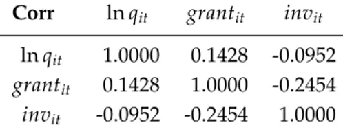
Table VIII. Correlation of equation residuals from OLS estimation, table VII

Corr ln qit grantit invit

ln qit 1.0000 0.1428 -0.0952

grantit 0.1428 1.0000 -0.2454

invit -0.0952 -0.2454 1.0000

With the restricted regression, like a ‘pooled’ regression, we capture both the

‘Within’ and the ‘Between’ variance. We can establish several main results from

table VII. First, we find that public capital is significant in the production

func-tion for all estimafunc-tions, i.e. the public capital expenditure of cities is productive.

Second, it turns out that autonomous investment by cities and grants from higher

level governments are complementary. Third, it appears that if the majority of the

city council’s allegiance is the same as the political affiliation of the ‘Bundesland’

government, the expected level of grants a city receives is higher. Fourth, tax

income has a positive effect on investment decisions, while the level of debts of

a given city has a negative impact. Fifth, the number of cars in a city also turns

out to be a significant determinant for infrastructure investment decisions. Sixth

and finally, in contrast to the findings from Cadot et al. (1999) for France, we do

not find evidence that the number of manufacturing firms in a given city has an

influence on infrastructure investment decisions. Thus, the crucial findings of the

’Between’ regression also hold for the restricted ’Within’ model.

The reported Hausman test statistic again favours the null hypothesis of no

simultaneity between infrastructure capital and output. Hence, feedback effects

from output on infrastructure via the investment equation appear to be weak.

5. Conclusions

In this study we estimated a system of equations comprising of a production

function, an infrastructure investment function and an investment grant function

using a panel data set of large German cities. Several key empirical findings

emerge from these estimates. First, we find that the public capital expenditure

of the cities in our sample are productive, i.e. public infrastructure is positively

linked with output of cities’ manufacturing sectors. Second, it appears that

in-frastructure investment and investment grants are complementary, i.e., there is

no evidence of a crowding out or substitutional effect from grants to cities

au-tonomous investment. Third, we find evidence that it is easier for a city to

ob-tain investment grants if the city council has the same political affiliation as the

higher-tier ‘Bundesland’ (state) government. Therefore, the allocation of grants

may depart substantially from an allocation that would be efficient and socially

optimal.

On the other hand, we do not find evidence that the number of

manufactur-ing firms is a significant determinant for the allocation of grants. This findmanufactur-ing is

in contrast to a previous study on French regions by Cadot et al. (1999). One

potential explanation for this is that in France the politically and socially highly

centralized system makes it easy for large firms to intervene in politics. The

hier-archy in administration mostly prevents the establishment of several autonomous

sub-levels in the decision making process.

The German case diverges from France in several aspects: overlapping

re-sponsibilities of governments, diluted accountability, mixed financing, and

ver-tical and horizontal coordination (Scharpf, 1999), which we summarized in this

study as ‘intertwined politics’. Our empirical estimations show that in those cases

where the local council members share the same political affiliation, they perform

better in attracting investment grants. Thus, political lobbying takes place but

only between different governmental levels. Because of the peculiar nature of the

bargaining process there is not much room for political lobbying by large firms.

Acknowledgements

We would like to thank Helmut Seitz for kindly providing us with parts of the city

panel data we use in this paper. Financial support from the Deutsche

Forschungs-gemeinschaft (DFG) for the project “Auswirkungen regionaler

Infrastrukturun-terschiede auf Produktivit¨at und Marktstruktur: Theorie und Evidenz f ¨ur

Deu-tschland und Frankreich” is gratefully acknowledged.

Notes

1_{These grants or subsidies from higher levels are called ‘Finanzzuweisungen’ (financial}

assign-ments). One major example in the infrastructure context is municipality transport infrastructure funds (‘GVFG’) that were created to promote transport infrastructure investment.

2_{This is not to say that in Germany powerful lobbying is not possible. It just adopts a different}

form. Individual firms which are having difficulties in lobbying for their own interests in a dis-tribution game still can unite to increase the overall investment budget. Therefore, organizations like the German Federation of Industries (BDI) participate vitally in infrastructure affairs. It is the typical form of interest representation in ’corporatist’ democracies (Lehmbruch, 1984).

3_{We assume that w}

iincludes both consumers’ and producers’ welfare. 4_{Original title: ‘Statistisches Jahrbuch der St¨adte und Gemeinden’.} 5_{This includes also the mining industries.}

6_{‘Volkswirtschaftliche Gesamtrechnung der L¨ander, Bruttowertsch ¨opfung der kreisfreien}

St¨ad-te, der Landkreise und der Arbeitsmarktregionen in der Bundesrepublik Deutschland’, Heft 26, Statistisches Landesamt Baden-W ¨urttemberg, 1995.

7_{For further details, see Deitmar (1993).}

8_{We would like to thank Helmut Seitz for kindly providing us with these data.}

References

Aaron, H. J. (1990). Discussion on D. A. Aschauer: Why is infrastructure important? In A. H. Munnell (Ed.), Is there a shortfall in public capital investment? Federal Reserve Bank of Boston, conference series no. 34: 51–63.

Ai, C. and S. P. Cassou (1997). On public capital analysis with state data. Economics Letters 57: 209–212.

Aschauer, D. A. (1988). Government spending and the falling rate of profit. Federal Reserve Bank

of Chicago, Economic Perspectives 12, May / June: 11–17.

Aschauer, D. A. (1989a). Is public expenditure productive? Journal of Monetary Economics 23: 177– 200.

Aschauer, D. A. (1989b). Does public capital crowd out private capital? Journal of Monetary

Economics 24: 178–235.

Aschauer, D. A. (1989c). Public investment and productivity growth in the Group of Seven.