Simulating the future impact of ICT on environmental sustainability: validating and recalibrating a system dynamics model - Background Data

(1)

ISSN: 1654-479X

TRITA-SUS 2014:3

KTH Centre for Sustainable Communications

M O H A M M A D A H M A D I A C H A C H L O U E I

L O R E N Z M . H I L T Y

Centre for Sustainable Communications

KTH, SE-100 44 Stockholm

www.cesc.kth.se

Simulating the future impact of ICT

on environmental sustainability

Working Paper - from the KTH Centre for Sustainable Communications

Stockholm, Sweden 2014

validating and re-calibrating a system dynamics model

- Background Data

(2)

Title: Simulating the future impact of ICT on environmental sustainability: validating and

re-calibrating a system dynamics model - Background Data

Authors:

Mohammad Ahmadi Achachlouei

Lorenz M. Hilty

Working Paper from KTH Centre for Sustainable Communications

ISSN: 1654-479x

TRITA-CSC-SUS Report 2014:3

(3)

2 Centre for Sustainable Communications (CESC)

The Centre for Sustainable Communications was established in 2007 by VINNOVA (The

Swedish Governmental Agency for Innovation Systems). CESC has established a strong

research environment at the KTH Royal Institute of Technology in collaboration with

several business partners, public authorities and civil organizations. As an interdisciplinary

research center CESC engage in innovative research in the field of ICT for sustainable

development that promote transformation of the society toward sustainable development.

Website:

http://cesc.kth.se

Partners 2012-2015

City of Stockholm

Coop

Ericsson

Swedish ICT - Interactive Institute

TeliaSonera

(4)

3

Abstract

This report serves as supplementary material to the book chapter, Modeling the Effects of ICT

on Environmental Sustainability: Revisiting a System Dynamics Model Developed for the

Eu-ropean Commission, published in ICT Innovations for Sustainability (edited by L. M. Hilty &

B. Aebischer. Springer, 2015). The current report was referred to in the book chapter

whenev-er the data to be presented exceeded the space provided for the book chaptwhenev-er.

(5)

4

Introduction

This report serves as supplementary material to the book chapter “Modeling the Effects of ICT on Environmen-tal Sustainability: Revisiting a System Dynamics Model Developed for the European Commission”

(Achachlouei and Hilty 2015)1 published in the book “ICT Innovations for Sustainability” (Hilty and Aebischer 2015)2. This report was referred to in the book chapter whenever the data to be presented exceeded the space provided for this chapter.

Achachlouei and Hilty (2015) revisited the assumptions and the results of a previous study commissioned in 2002 by the European Commission’s Institute for Prospective Technological Studies (IPTS) to explore the cur-rent and future environmental effects of ICT. The aim of that study (here called “the IPTS study”) was to esti-mate positive and negative effects of the ICT on environmental indicators with a time horizon of 20 years. The method applied was to develop future scenarios, build a model based on the SD approach, validate the model and use it to run quantitative simulations of the scenarios.

This report, which provides supplementary material for the book chapter (Achachlouei and Hilty 2015), is orga-nized into four sections:

1. Overview of original and new scenarios 2. New assumptions based on empirical data 3. New simulated trends compared to empirical data 4. New simulation results compared to original results

1_{Achachlouei, M. A., & Hilty, L. M. (2015). Modeling the Effects of ICT on Environmental Sustainability: Revisiting a}

System Dynamics Model Developed for the European Commission. In ICT Innovations for Sustainability (pp. 449-474). Springer International Publishing.

2_{Hilty, L. M., & Aebischer, B. (2015). ICT Innovations for Sustainability. Advances in Intelligent Systems and}

(6)

5

1. Overview of Old and New Scenarios

Original assumptions in 2003: Scenarios A, B, and C

3

The task of the original study was to make a prediction about the future effect of ICT on environmental sustaina-bility. When building the System Dynamics model, it soon became clear that this prediction would depend on conditions that were external to the model, called “external factors,” in particular: the development of the general economic activity level (usually represented by the Gross Domestic Product, GDP), the labor market, energy prices, the climate for innovation, the general attitude of the population toward ICT and toward environmental issues, spatial dispersion, and the speed of some technological developments.

Given the fundamental difficulty to forecast these factors over 20 years, the project team applied a scenario ap-proach to deal with the uncertainty. In expert and stakeholder workshops, three possible futures were developed in the form of scenarios, each of them representing a development that was internally consistent and plausible according to the participants’ assessment. Brief descriptions of the original scenarios are repeated here [4]:

• Scenario A, called “Technocracy,” was characterized by strong economic growth, leading to an in-crease in the workforce which is also reflected in an inin-crease in desk workers due to the service-based nature of the economy. Strong growth also leads to a significant increase in the total number of households and buildings due to increased economic activity. Collusion between government and business in determining the framework for business activity is dominated by large companies, which is reflected in a fall in the number of SMEs.

• Scenario B, called “Government first,” was characterized by weak economic growth which is re-flected in the lack of growth in the number of households, buildings, and desk workers. The total labor force decreases due to stagnating economic growth and the flight of industry from Europe. The settlement pattern becomes more dispersed due to the development and high take-up of envi-ronmental and social applications of technology, for example ITSs, smart homes, and virtual con-ferencing. This also leads to an increase in the percentage of SMEs.

• Scenario C, called “Stakeholder democracy,” was characterized by steady economic growth, lead-ing to an increase in the number of households and desk workers and the total labor force. A reduc-tion in the levels of inequality between the developed and developing worlds and the expansion of the EU to 35 Member States reduce immigration to Europe and, as a result, the expected rise in population does not materialize. The settlement pattern becomes more dispersed due to business in-vestment in applications that can improve virtual conferencing and smart home technologies.

New assumptions in 2014 based on empirical data: Scenario D

The new Scenario D is directly based on empirical data (see Table S-1): For the years 2000-2012, statistical time series were used, and for 2013-2020, the CAGR values drawn from this data (also shown in Table S-1) were used for trend extrapolation.

(7)

6

2. New assumptions based on empirical data

Table S-1 presents more details on the empirical data (more details on Table 1 in Achachlouei and Hilty 2015) for EU-15 over 2000-2012: both time-series values and CAGR4 values (CAGR values were used when the data were missing for some years between 2000 and 2013. They were also used as estimates for 2013-2020). The val-ues in Table S-1 were used as assumptions in the new scenario (D).

Table S-1: Empirical data for EU15 over 2000-2012 used as assumptions in Scenario D No External

variable

Empirical data for EU15 2000-2012 2001 2002 2003 2004 2005 2006 2007 2008 2009 2010 2011 2012 2013 2014 2015 2016 2017 2018 2019 2020 M2 GDP Annual Growth Rate 1.11 % (14.2% increase over 2000-2012) 2.0 1.2 1.3 2.4 2.0 3.2 3.0 0.1 -4.6 2.0 1.5 -0.5 1.11 1.11 1.11 1.11 1.11 1.11 1.11 1.11 M4 Labor Demand Annual Growth Rate 0.67 % (8.3% increase over 2000-2012) 1.47 0.69 1.01 0.86 1.56 1.84 1.75 0.96 -1.76 -0.41 0.40 -0.33 0.67 0.67 0.67 0.67 0.67 0.67 0.67 0.67 M7 Population Annu-al Growth Rate 0.46 % (5.7% increase over 2000-2012) 0.46 0.55 0.61 0.64 0.61 0.58 0.63 0.58 0.44 0.40 0.39 -0.39 0.46 0.46 0.46 0.46 0.46 0.46 0.46 0.46 M9 Number of Households An-nual Growth Rate

1.51 % for 2005-12 (11.1% increase over 2005-2012) 1.51 1.51 1.51 1.51 1.51 2.42 1.03 0.99 3.36 0.94 1.24 0.62 1.51 1.51 1.51 1.51 1.51 1.51 1.51 1.51 M15 Number of SMEs Annual Growth Rate 0.78% for 2005-12 (5.6% increase over 2005-2012) 0.78 0.78 0.78 0.78 0.78 0.78 0.78 0.78 -1.28 3.76 -0.76 -2.20 0.82 3.10 0.78 0.78 0.78 0.78 0.78 0.78 M16 Office Work

De-mand Annual Growth Rate 1.28 % for 2008-2011 1.28 1.28 1.28 1.28 1.28 1.28 1.28 1.28 1.28 1.28 1.28 1.28 1.28 1.28 1.28 1.28 1.28 1.28 1.28 1.28 E400 Fossil Energy

Price Annual Change Rate

2.8 % Automotive gas oil price as

proxy

CAGR over 2000-2012 is about 2.8%

U400 Shift to Energy-Efficient ICT Half-life ~ 7.5 a ~ 7.5 a T400 ICT-Induced Spa-tial Settlement Dispersion 20% increase in average commuting distance over the period 2000-2010 in Finland

as proxy

25% over the period 2000-2020

Since the empirical proxy indicator shows a growth of 20% over the period 2000-2010, we chose to use the assumption made in Scenario B and C, which

was a growth of 25% estimated over the period 2000-2020. E12 D&T Electricity

Use Efficiency Potential ~ 30 a (7.9% increase in efficiency over 9 years 2000-2009 in EU-27) E12=50%, f(t)=E12*(1-(0.5^(t/E13)))

Given 7.9% increase in efficiency over 9 years 2000-2009, f(9)=7.9%, E13 is about 30 years

E13 D&T Electricity Use Efficiency Half-life E17 D&T Electricity

Price Annual Growth Rate 3.9 % (35% increase over 2005-2013) 3.9 3.9 3.9 3.9 5.43 9.83 0.43 4.07 -0.41 5.16 4.21 2.54 3.9 3.9 3.9 3.9 3.9 3.9 3.9 3.9 E19 Electricity Supply

Efficiency

Poten-tial ~ 20 a

(7.1% increase in efficiency over 10 years 2000-2010)

E19=25%, f(t)=E19*(1-(0.5^(t/E20)))

Given 7.1% increase in efficiency over 10 years 2000-2010, f(10)=7.1%, E20 is closer to 20 years (as assumed in Scenario A and C) E20 Electricity Supply

Efficiency Half-life

(8)

7

U201 Average Useful Life of ICT An-nual Change Rate

-7.3% over 8 years 2000-2008 - W31 MSW Recycling Potential _{~ 10 a} (28% recycling rate in 2011) W31=53%, f(t)=W31*(1-(0.5^(t/W32)),

Given 28% for recycling rate in 2011, f(11)=28%, W32 is about 10 years W32 MSW Recycling

(9)

8

3. New simulated trends compared to empirical data

This section provides more comparisons between the simulated trends in the new scenario (D) and the real-world trends observed over 2000-2011. This is related to the following research question addressed in Section 6 in the book chapter (Achachlouei and Hilty 2015):

RQ2: Are the main trends (in energy, transport, etc., as shown in Figures 6-2, 6-3, 6-4, 6-5, 6-6, 6-7, 6-8, and 6-9 in Hilty et al. 2004) that the IPTS model predicts for a realistic scenario consistent with the currently avail-able data?

Since none of the three scenarios dominantly represents the reality over the past years, we defined a new scenar-io (Scenarscenar-io D) based on the empirical data available today. Figures S-1, S-2, S-3, S-4, S-5 and S-6 show select-ed trends in energy, transport, and waste, electricity consumption, greenhouse gas emissions, and modal split in passenger transport, comparing the simulated development in Scenario D with the real world trends.

As shown in Figures S-1, S-2, S-3, S-4, S-5 and S-6, the predictions were roughly plausible, but cannot be taken as precise predictions, which is not surprising because the purpose of the model was not to predict the develop-ment of transport and energy demand and other environdevelop-mental indicators in absolute terms, but the relative im-pact of ICT on these indicators.

Fig. S-1. Comparison of simulated trends (Scenario D, mean sub-scenario) with empirical trends5 of: freight transport per-formance (“F Transp Index”) and passenger transport perper-formance (“P Transp Index”), compared to GDP index. (2000 = 100 %)

5_{European Commission: Statistical pocketbook 2013,}

http://ec.europa.eu/transport/facts-fundings/statistics/pocketbook-2013_en.htm

Simulated trends 2000-2020

Empirical trends 2000-2011

(10)

9

Fig. S-2. Comparison of simulated trends (Scenario D) with empirical trends6 of: energy consumption by the sectors transport, domestic and tertiary, and industry. Abbreviations: PJ: Petajoule; D&T: Domestic and tertiary sector.

Fig. S-3. Comparison of simulated trends (Scenario D) with empirical trends7 of: municipal solid waste (MSW), the recycling rate, and the e-waste fraction in megatonnes (Mt).

6

Eurostat: Supply, transformation, consumption - all products - annual data. Product code: nrg_100a (2013)

7_{Eurostat: EuroStat: Municipal waste. Product code: env_wasmun (2014)}

Eurostat: Waste Electrical and Electronic Equipment (WEEE). Product code: env_waselee (2014)

Simulated trends 2000-2020 Empirical trends 2000-2011 Simulated trends 2000-2020 Empirical trends 2000-2011

(11)

10 Fig. S-4.Comparison of simulated trends (Scenario D) with empirical trends8 of energy consumption

Fig. S-5.Comparison of simulated trends (Scenario D) with empirical trends9_{of total electricity}

Fig. S-6.Comparison of simulated trends (Scenario D) with empirical trends10_{of passenger transport performance by traffic}

mode (Note: empirical trend for air passenger transport is missing). Abbreviations: Gpkm=109 passenger-kilometer, PCar=Privat car, BusC=Bus and Coach, TraM=Tram and Metro.

8_{Eurostat: Supply, transformation, consumption - all products - annual data. Product code: nrg_100a (2013)} 9_REF??? Simulated trends 2000-2020 Empirical trends 2000-2011 Simulated trends 2000-2020 Empirical trends 2000-2011 Simulated trends 2000-2020 Empirical trends 2000-2011

(12)

11

4. New simulation results compared to original results

This section presents quantitative results of the simulation modeling using the new assumptions described in Ta-ble S-1 (Scenario D). Simulation results for Scenario D are compared with the results for the original three sce-narios (A, B, and C).

For each scenario, the results for three sub-scenarios are presented. These sub-scenarios express best-case, worst-case, and mean assumptions about model parameters that were specified with a range of uncertainty. The “mean” sub-scenarios simply used the arithmetic mean of the best- and worst-case values of each (input) parameter. Moreover, for each scenario, the results for two versions of simulation runs are presented: the reference (or regu-lar) run and the “ICT Freeze” run. The reference run simulates the development of ICT as it is predicted over the simulation period. The “ICT Freeze” run “freezes” ICT diffusion and use at the level of the year 2000.

In this section we revisit the results presented

Table 1. Simulated values in Scenario D for environmental indicators divided by GDP in the year 2020, expressed in % of the values of the year 2000. This table provides updated results compared to Table 4 in Hilty et al. (2006) Initial 1.1.2001 D worst 1.1.2021 D mean 1.1.2021 D best 1.1.2021

Energy intensity Reference Run 398.91951 77.6% 71.1% 61.6%

ICT Freeze 82.2% 78.7% 75.3%

GHG intensity Reference Run 33.746827 62.6% 63.2% 51.3%

ICT Freeze 77.4% 71.3% 65.0%

Material intensity Reference Run 1.88 87.0% 74.2% 56.4%

ICT Freeze 77.5% 73.6% 69.3%

Freight transport intensity Reference Run 1 114.6% 105.2% 84.6%

ICT Freeze 115.8% 110.3% 104.0%

Passenger transport intensity Reference Run 1 111.9% 108.6% 103.8%

ICT Freeze 108.3% 103.5% 99.5%

Table 2. Simulated results for Scenario D in energy consumption by the sectors transport, domestic and tertiary, and industry. Compare this with original scenarios in Table 6-1 in Hilty et al (2004).

Initial 1.1.2001 D worst 1.1.2021 D mean 1.1.2021 D best 1.1.2021

Total Energy PJ Reference Run 39892 38642 35408 30654

ICT Freeze 40927 39177 37468

Transport Energy PJ -- Reference Run 12854 15104 14110 12496

ICT Freeze 15425 14486 13677

D&T Energy PJ -- Reference Run 15666 13633 12876 12660

ICT Freeze 14441 14716 14942

Industrial Energy PJ Reference Run 11372 9905 8423 5499

ICT Freeze 11061 9976 8848

(13)

12

Table 3. Simulated results for Scenario D in electricity consumption, total and for ICT. Compare this with original scenarios in Fig 6-3 in Hilty et al (2004).

Total Electricity PJ Reference Run 8020 8501 8608 9014

ICT Freeze 7814 8198 8554

ICT Electricity PJ Reference Run 519 1520 966 623

ICT Freeze 519 519 519

Table 4. Simulated results for Scenario D in energy-related greenhouse gas emissions by the sectors transport, domestic and tertiary, and industry. Compare this with the results of original scenarios in Ta-ble 6-1 in Hilty et al (2004). Initial 1.1.2001 D worst 1.1.2021 D mean 1.1.2021 D best 1.1.2021

Total GHG Mt Reference Run 3375 2638 2663 2162

ICT Freeze 3262 3005 2738

Transport GHG Mt Reference Run 905 1054 996 881

ICT Freeze 1082 1017 958

D&T GHG Mt Reference Run 1507 980 1096 971

ICT Freeze 1319 1269 1196

Industry GHG Mt Reference Run 963 604 571 310

Table 5. Simulated development of freight transport performance (tkm) compared to GDP and passenger transport performance in Scenario D (Compare with Fig 6-8 in Hilty et al 2004).

99 GDP Index Reference Run 100.0 124.8 124.8 124.8

ICT Freeze 124.8 124.8 124.8

01 F Transp Index Reference Run 100.0 143.0 131.3 105.6

ICT Freeze 144.5 137.6 129.8

02 P Transp Index Reference Run 100.0 139.7 135.6 129.6

ICT Freeze 135.1 129.1 124.2

07 MSW not recycled Index Reference Run 100.0 80.2 68.4 52.1

ICT Freeze 71.4 68.7 64.7

08 Materials Index Reference Run 100.0 86.1 79.4 64.1

(14)

13

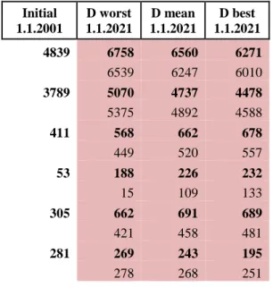
Table 6. Simulated development of passenger transport in 109 passenger km for private car (PCar), bus

and coach (BusC), tram and metro (TraM), train, and air transport in Scenario D. (Compare with Fig 6-6 in Hilty et al 2004). Initial 1.1.2001 D worst 1.1.2021 D mean 1.1.2021 D best 1.1.2021

Total Gpkm Reference Run 4839 6758 6560 6271

ICT Freeze 6539 6247 6010

PCar Gpkm Reference Run 3789 5070 4737 4478

ICT Freeze 5375 4892 4588

BusC Gpkm Reference Run 411 568 662 678

TraM Gpkm Reference Run 53 188 226 232

Train Gpkm Reference Run 305 662 691 689

Air Gpkm Reference Run 281 269 243 195

Table 7. Simulated results of municipal solid waste (MSW), the recycling rate and the e-waste fraction in Mt. in Scenario D. The second table shows the same variables and the GDP for comparison as an index with 100 % in 2000. (Compare with Fig 6-9 in Hilty et al 2004)

Total MSW Mt Reference Run 188.00 204.02 174.09 132.43

ICT Freeze 181.73 172.67 162.63

Recycled MSW Mt Reference Run 38.92 84.47 72.07 54.83

ICT Freeze 75.24 70.28 66.19

E-Waste Mt Reference Run 8.13 56.25 38.57 25.78

ICT Freeze 0.80 0.80 0.80

Waste not recycled Mt Reference Run 149.08 119.56 102.01 77.60

ICT Freeze 106.49 102.39 96.44 Initial 1.1.2001 D worst 1.1.2021 D mean 1.1.2021 D best 1.1.2021

99 GDP Index Reference Run 100 124.8 124.8 124.8

ICT Freeze 124.8 124.8 124.8

16 Total MSW Index Reference Run 100 108.5 92.6 70.4

ICT Freeze 96.7 91.8 86.5

17 Recycled Index Reference Run 100 217.0 185.2 140.9

ICT Freeze 193.3 180.6 170.1

18 E-waste Index Reference Run 100 691.5 474.2 317.0

(15)

14

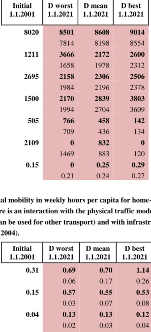
Table 8. Simulated results in Scenario D for the electricity mix. CHP is not included because it is not an energy source, but a way of using the heat that is produced in some modes of power generation (usually natural gas). Compare with Fig 6-5 in Hilty et al (2004).

Electricity PJ Reference Run 8020 8501 8608 9014

ICT Freeze 7814 8198 8554

Renewables PJ Reference Run 1211 3666 2172 2600

ICT Freeze 1658 1978 2312

Nuclear PJ Reference Run 2695 2158 2306 2506

ICT Freeze 1984 2196 2378

Natural Gas PJ Reference Run 1500 2170 2839 3803

ICT Freeze 1994 2704 3609

Oil Products PJ Reference Run 505 766 458 142

Solid Fuels PJ Reference Run 2109 0 832 0

ICT Freeze 1469 883 120

RES share in electricity Reference Run 0.15 0 0.25 0.29

ICT Freeze 0.21 0.24 0.27

Table 9. Simulated results in Scenario D for virtual mobility in weekly hours per capita for home-based telework, teleshopping and virtual meetings. There is an interaction with the physical traffic modes through the time budget constraint (saved time can be used for other transport) and with infrastructure capacity. Compare with Figure 6-7 in Hilty et al (2004).

Telework h Reference Run 0.31 0.69 0.70 1.14

ICT Freeze 0.06 0.17 0.26

Teleshopping h Reference Run 0.15 0.57 0.55 0.53

ICT Freeze 0.03 0.07 0.08

V Meetings h Reference Run 0.04 0.13 0.13 0.12

ICT Freeze 0.02 0.03 0.04

Telework pkmE Reference Run 1.5E+10 3.7E+10 3.8E+10 6.1E+10

ICT Freeze 3.05E+09 9.33E+09 1.37E+10 Teleshopping pkmE Reference Run 5.88E+10 2.4E+11 2.4E+11 2.3E+11

ICT Freeze 1.24E+10 2.88E+10 3.29E+10 V Meetings pkmE Reference Run 1.29E+11 4.1E+11 4E+11 4E+11

ICT Freeze 7.3E+10 9.71E+10 1.19E+11

(16)

15

Hilty, L.M., Arnfalk, P., Erdmann, L., Goodman, J., Lehmann, M., Wäger, P. (2006) The relevance of infor-mation and communication technologies for environmental sustainability—a prospective simulation study. Envi-ron. Modell. Softw. 11(21), 1618–1629.

Hilty, L.M., Wäger, P., Lehmann, M., Hischier, R., Ruddy, T.F., Binswanger, M. (2004). The future impact of ICT on environmental sustainability. Fourth interim report. Refinement and quantification. Institute for Prospec-tive Technological Studies (IPTS), Sevilla.

Achachlouei, M. A., & Hilty, L. M. (2015). Modeling the Effects of ICT on Environmental Sustainability: Re-visiting a System Dynamics Model Developed for the European Commission. In ICT Innovations for Sustaina-bility (pp. 449-474). Springer International Publishing.

Hilty, L. M., & Aebischer, B. (2015). ICT Innovations for Sustainability. Advances in Intelligent Systems and Compu-ting. Springer International Publishing.