Size Optimization of Constructed Wetlands for
Phosphorus Retention in Agricultural Areas
Size Optimization of Constructed Wetlands for Phosphorus
Retention in Agricultural Areas
Anna Ferguson
Supervisor: Pia Geranmayeh, Department of Aquatic Sciences and Assessment, SLU Assistant supervisor: Faruk Djodjic, Department of Aquatic Sciences and Assessment, SLU Examiner: Helena Aronsson, Department of Soil and Environment, SLU
Credits: 30 ECTS Level: Second cycle, A2E
Course title: Master thesis in Soil science, A2E – Agrictulture Programme Soil/Plant Course code: EX0881
Programme/Education: Agriculture programme – Soil and Plant Sciences 270 credits (Agronomprogrammet – mark/växt 270 hp)
Course coordinating department: Soil and Environment Place of publication: Uppsala
Year of publication: 2019
Title of series: Examensarbeten, Institutionen för mark och miljö Number of part of series: 2019:08
Online publication: http://stud.epsilon.slu.se
Abstract
Eutrophication is one of the main threats to the Baltic Sea and Sweden is not expected to reach its environmental target of No Eutrophication by 2020. Phosphorus (P) loss from terrestrial systems is one of the principal causes of eutrophication in water re-cipients and the need to decrease P loss from agricultural land is pressing. One way to reduce P losses from agricultural areas is by constructing wetlands (CW), with sedimentation as the primary process for P reduction. The efficiency of CWs is de-pendent on several factors regarding P load and hydraulic load (HL), which to a high degree is governed by CW area and shape as well as catchment area and land use distribution. Today, the most common method of estimating catchment area is to use low-resolution topography maps. There is an increasing availability of digital eleva-tion models (DEM) and databases that could aid the planning process of CWs by better estimating their catchment size and potential efficiency.
The DEM of 2x2 m has been used to determine catchment areas of 39 CWs, show-ing that catchments are on average 8 % larger compared to earlier estimations based on low-resolution maps. Orthophotographs have been used to calculate current CW areas, to determine the ratio between wetland and catchment area (AW:AC). Using
existing data on P accumulation in 8 previously studied CWs, the relation to several catchment and wetland factors was studied. Modelled runoff data from SMHI was used to calculate annual average, maximum and 95th percentiles of HL. Land use distribution in the associated catchments was determined using data from HELCOMs sixth pollution load compilation (PLC-6) as well as textural soil distributions of ara-ble land from the Digital Araara-ble Soil Map of Sweden (DSMS). The best modelled HL for estimation of P accumulation was long-term annual average (R2 = 0.93; p = 0.0006). However, trends were also found between accumulated P and other catch-ment factors. Multiple regression analyses showed that HL, AW:AC, and share of
ar-able land within the catchment can be used to estimate CW efficiency in terms of potential P accumulated per CW area and year (R2 = 0.77; p = 0.03). However, the multiple regression analysis also showed that it is difficult to determine optimum values of studied parameters as they can compensate for one another. The result of the regression analysis was used to predict the P retention of a total of 39 CWs, show-ing a high variation of potential P accumulation, indicatshow-ing the usefulness of estimat-ing the potential P retention prior to construction to optimize CW size and location.
Sammanfattning
Övergödning är ett av de främsta hoten mot Östersjöns vattenkvalitet och Sverige förväntas inte nå miljömålet Ingen övergödning tills år 2020. Fosfor (P) -förluster från marken är en av de främsta orsakerna till övergödning i vatten och behovet av att minska P-förluster från jordbruksmark ökar. Ett sätt att minska P-förluster från jordbruksområden är att anlägga våtmarker, där sedimentering antas vara den huvud-sakliga processen för P-reduktion. P- och hydraulisk belastning (HL), som i hög grad styrs av våtmarkens storlek och utformning, samt avrinningsområdets storlek och markanvändning, är avgörande för effektiviteten av våtmarker. Idag är den vanligaste metoden för att uppskatta avrinningsområdet att använda topografiska kartor med re-lativt låg upplösning. Det finns en ökad tillgänglighet av digitala höjdmodeller (DEM) och databaser som skulle kunna hjälpa planeringsprocessen av våtmarksan-läggning genom att bättre uppskatta deras avrinningsområden och därmed även po-tentiella effektivitet.
Högupplöst DEM (2x2 m) har använts för att bestämma avrinningsområden för 39 våtmarker, och visade att avrinningsområden i genomsnitt är 8 % större än vad som tidigare uppskattats med hjälp av kartor med lägre upplösning. Ortofoton har använts för att beräkna aktuella våtmarksområden för att bestämma förhållandet mellan våt-mark och avrinningsområde (AW:AC). Genom att använda befintliga data för
P-ack-umulering i 8 tidigare undersökta våtmarker, studerades förhållandet mellan olika faktorer för avrinningsområden och våtmarker. Modellerad avrinning från SMHI an-vändes för att beräkna årsmedel, maximala och 95:e percentiler av HL. Fördelning av markanvändning i avrinningsområden bestämdes med hjälp av data från HELCOMs sjätte Pollution load compilation (PLC-6). Kornstrorleksfördelningar inom jordbruksmark uppskattades med hjälp av den digitala åkermarkskartan (DSMS). Långsiktigt årligt genomsnittlig HL var den bästa av de modellerade HL för uppskatta P-ackumulering (R2 = 0,93; p = 0,0006), men trender kunde också ses mellan ackumulerad P och andra faktorer. Multipla regressionsanalyser visade att HL, AW:AC och andel jordbruksmark i avrinningsområdet kan användas för att
upp-skatta våtmarkseffektiviteten med avseende på potentiell P ackumulering per våt-marksyta och år (R2 = 0,77; p = 0,03). Den multipla regressionsanalysen visade emel-lertid också att det är svårt att bestämma optimala värden av studerade parametrar eftersom de kan kompensera för varandra. Resultatet av analysen användes för att uppskatta P-retentionen av totalt 39 våtmarker. Variationen av potentiell P-ackumu-lation var stor, vilket belyser vikten av att uppskatta den potentiella P-retentionen före anläggning för att optimera våtmarkens storlek och plats.
Övergödning är en process som kan ske när det blir ett tillskott av näringsämnen i vattendrag. Tillskottet leder till tillväxt av bland annat alger, vilket förändrar ekosy-stemet i vattendraget och kan leda till försämrad vattenkvalitet. Östersjön är kraftigt övergödd och flera internationella och nationella insatser arbetar för att minska nä-ringsläckaget från land till vatten. Ett av Sveriges miljömål är Ingen Övergödning, detta förväntas dock inte att uppnås till år 2020. Fosfor (P) -förluster från marken är en av de främsta orsakerna till övergödning. Detta då P är ett av de mest begränsade näringsämnena i akvatiska ekosystem, varpå tillskott möjliggör tillväxt. Totalt sett bidrar mänskliga aktiviteter med ca 34 % av de totala P-förlusterna till Östersjön. Jordbruket är en av de största källorna och står för ungefär 14 % av de totala förlus-terna. Ett sätt att minska P-förluster från jordbruksområden är att anlägga våtmarker i kanten av åkermark och på så vis fånga P innan den försvinner ut i vattnet. Den mesta P är bunden till partiklar, som sjunker till botten (sedimenterar) i våtmarken och därmed hindras från att föras vidare.
Flera faktorer påverkar sedimentationen. Avrinningsområdet till en våtmark, det vill säga området vars vatten rinner ut i våtmarken, påverkar hur väl våtmarken fun-gerar, både genom vad det innefattar och genom sin storlek. Jordbruksmark har ge-nerellt högre P-förluster jämfört med till exempel skog. Även marktyp kan påverka P förluster då mer P kan binda till lera jämfört med exempelvis sandjordar. Storleken på området är avgörande för hur mycket vatten som kommer till våtmarken. Det är nödvändigt att det kommer tillräckligt med vatten till våtmarken för att den ska fun-gera över huvud taget, samtidigt är det viktigt att det inte kommer för mycket, så P i våtmarken har tid att sedimentera. Det är således viktigt att veta avrinningsområdets storlek och vad det innehåller för att kunna designa en våtmark så den effektivt kan ansamla P från området.
Denna studie har undersökt hur digitala höjdmodeller (DEM) med hög upplösning kan användas för att uppskatta avrinningsområden till våtmarker och sett hur upp-skattningarna skiljer sig från tidigare bedömningar gjorda med den vanligare meto-den, topografiska kartor med lägre upplösning. Därefter har studien använt data från tidigare forskning av åtta våtmarker för att se relationer mellan faktorer som påverkar våtmarkernas effektivitet av att ansamla P. Mängden vatten som nått våtmarken be-räknades som modellerad hydraulisk belastning (HL), det vill säga mängden vatten fördelat på våtmarksytan, både vid maximalt- och medelflöde, för att se om det fanns någon skillnad i hur de relaterar till uppsamlad P. Slutligen slogs flera faktorer rö-rande marktyp, markanvändning, utformning av våtmarken samt storleken av både våtmark och avrinningsområde ihop, för att sedan beräkna den potentiella P-uppsam-lingen i befintliga våtmarker.
Det visade sig att DEM-estimerade avrinningsområden var generellt 8 % större än de tidigare uppskattningarna, och att den utökade delen främst bestod av skogspartier
Populärvetenskaplig sammanfattning
eller annan mark än åkermark. Detta kan vara dubbelt så negativt för P-uppsamling eftersom ett större område kommer leda till mer vatten i våtmarken, samtidigt som det finns relativt lägre mängd P i området. En mindre mängd P kommer alltså ha mindre tid att sedimentera i våtmarken. Studien visade att det inte var någon större skillnad i hur maximalt HL och långtidsmedel (1999–2017) HL relaterade till P-upp-samling, varpå det är bäst att använda lång-tidsmedel för att utvärdera mönster mellan P-uppsamling och HL. Däremot är studien baserad på enbart 8 våtmarker och resul-taten är osäkra.
När flera faktorer slogs ihop för att beräkna den potentiella P-uppsamlingen visade sig HL, andelen jordbruksmark i avrinningsområdet samt AW:AC, relationen mellan
storleken på våtmarken och storleken på avrinningsområdet, att vara de viktigaste faktorerna. Den potentiella P-uppsamlingen beräknades för totalt 39 våtmarker. Fem-ton våtmarker beräknades till att inte kunna samla P, på grund av att antingen för lite eller för mycket vatten tillkom. Studien visade att flera faktorer påverkar P-uppsam-ling, både positivt och negativt, vilket gör det svårt att sätta ramverk som skulle kunna hjälpa vid våtmarksanläggning, men vissa mönster kunde urskiljas. Den hydrauliska belastningen bör absolut inte vara lägre än 35 eller över 310 meter per år och AW:AC
bör hållas mellan 0,07–0,35 % för bäst effektivitet, det vill säga mest uppsamlad P per våtmarksyta. Andelen jordbruksmark kan variera men eftersom syftet med våt-markerna är att hindra P-förluster från just jordbruksmark bör andelen i avrinnings-området vara så stor som möjligt.
Informationen som erhållits av studien kan vara till nytta vid våtmarksanläggning då den visar vikten av att noggrant uppskatta avrinningsområdet och vad det innefat-tar, för att kunna veta vart våtmarken bör anläggas samt hur stor våtmarken bör vara för att samla upp P innan det når känsliga vattendrag.
List of tables 7 List of figures 8 Abbreviations 9 1 Introduction 10 1.1 Background 10 1.2 Constructed wetlands 11 1.3 Aims 12
2 Materials and methods 14
2.1 Wetland descriptions 14
2.2 Catchment characteristics 16
2.2.1 Catchment area 16
2.2.2 Wetland area and length to width ratio 17
2.2.3 Soil texture and classification 17
2.2.4 Land use distribution 18
2.3 Modelled loads 18
2.3.1 Hydraulic load 18
2.3.2 Flow accumulation of particles 19
2.4 Software and statistical analysis 19
3 Results 21
3.1 Comparisons of areas estimated using different tools 21
3.1.1 Areas of wetlands and catchments 21
3.1.2 Land use distribution 23
3.2 Phosphorus accumulation 24
3.2.1 Annual versus extreme modelled hydraulic loads 24 3.2.2 Wetland size in relation to catchments and wetland shape 27 3.2.3 Soil texture and particle-size distribution on arable land 28
3.3 Potential P retention 29
4 Discussion 32
4.1 Using different tools to estimate catchment areas 32
4.2 Phosphorus accumulation and hydraulic load 33
4.3 Potential phosphorus retention 35
5 Conclusions 37 6 Future research 38 References 39 Acknowledgements 42 Appendix 1 43 Appendix 2 45 Appendix 3 47 Appendix 4 48
Table 1. Characteristics of 8 previously studied CWs, showing year of construction, estimated areas of CW (AWE) and catchment (ACE), ratio between CW area and catchment area (AW:AC),
length-width ratio (L:W), hydraulic load (HL), sediment accumulation and specific P retention (Kynkäänniemi 2014). 14 Table 2. Comparison between previously determined CW area (AWE), orthophoto determined CW area
(AWO), previously estimated catchment areas (ACE) and DEM determined catchments from
point of inflow (ACDEM) and outflow (ACDout). Minimum and maximum differences are shown
as absolute %. 22
Table 3. Wetland to catchment area ratios of 8 wetlands using previously estimated values only (AWE:ACE), estimated wetland area and DEM determined catchments (AWE:ACDEM) and
orthophoto determined wetland areas and DEM determined catchment (AWO:ACDEM).23
Table 4. Polynomial fit of 8 wetlands P accumulation and modelled hydraulic load (HL) using ACDEM and
AWO, and previously used data of short-term (2-3 years) average HL (Kynkäänniemi, 2014).
Modelled HL-data of mean, maximum and 95th percentile of monthly and annual average
was obtained for the time periods 1999-2017 (long-term), 1999-construction year and construction-2017 (CW life-time) from SMHIs water web (SMHI, 2019). One CW was constructed 1997 and thus not included in some time periods. Max HL and P accumulated is the vertex point of the polynomial fit. 25
Figure 1. Geographical location of the 39 wetlands, situated in the south of Sweden. The eight
previously studied wetlands are marked as triangles. 15
Figure 2. Comparison of DEM determined and estimated catchment area (ha) of 38 wetlands. Color
range indicates absolute difference between the areas (%), the line shows 1:1 relationship. 22
Figure 3. Previously estimated agricultural land (%) versus agricultural land in 22 DEM determined
catchments using land use data from PLC-6 (Widén-Nilsson et al. 2016). Size of markers indicates relative size of DEM catchment. The line represents 1:1 relationship. 24
Figure 4. P accumulation in eight wetlands and hydraulic load (HL) as short-term average used by
Kynkäänniemi (2014) (circle), modelled long-term average (square) and long-term
maximum (cross). 26
Figure 5. Phosphorous accumulation determined by Kynkäänniemi (2014) in 8 wetlands in relation to
hydraulic load (HL) used by Kynkäänniemi (2014) (linear fit, R2 = 0.74, n = 6) and modelled
long-term average (polynomial fit R2 = 0.93, n = 8). Modelled HL is based on catchment
areas determined using DEM and wetland areas determined using orthophotos. 26
Figure 6. Distribution of the modelled long-term average hydraulic loads for 39 wetlands. Striped area
shows the 8 previously studied, solid shows the 31 added wetlands. 27
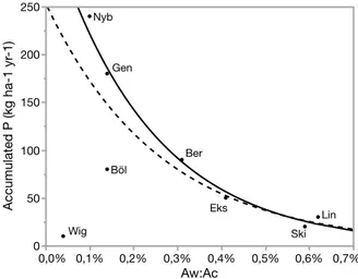
Figure 7. AWO:ACDEM in relation to accumulated phosphorus in the 8 wetlands. Dashed line R2 = 0.83; p
= 0.0027 (excluding Wig). Solid line R2 = 0.96; p= 0.0005 (excluding Wig and Böl).28
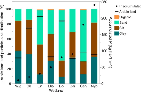
Figure 8. Soil particle-size distribution of the arable land within the catchments of eight wetlands and
their respective accumulated phosphorus. Horizontal lines show arable land (%) within the
catchment. 29
Figure 9. Principal components analysis showing how factors relate to P accumulated (kg P ha-1 yr-1)
and to each other. 30
Figure 10. Potential phosphorus accumulation > -50 kg P ha-1 yr-1. Several CWs were calculated to
have negative P retention, most of which are not shown in this graph. Polynomial fit calculated 4 CWs to be negative, 5- and 3-factor multiple regression (MRA) equations calculated 14 and 15 CWs, respectively, to have a negative P accumulation. 31
ACDEM Catchment delineated using digital elevation model, to point of inflow ACDout Catchment delineated using digital elevation model, to point of outflow ACE Previously estimated catchment area based on lower resolution
topogra-phy maps
AW:AC Ratio between wetland area to catchment area AWE Wetland area previously estimated
AWO Wetland area determined from orthophotograph CW Constructed wetland
DSMS Digital arable soil map of Sweden HL Hydraulic load
L:W Length to width ratio, length from inlet to outlet, divided by average width measured every 10 m.
WRT Water residence time
1.1 Background
Eutrophication is one of the main threats to the water quality of lakes and water-courses around Sweden. As of 2018, nearly the entire Baltic Sea was judged to be in a state of eutrophication (SEPA 2019). Eutrophication is primarily caused by ex-cessive loading of nutrients, leading to a growth burst of algae. During the exex-cessive growth, oligotrophic species are at risk of dying out, with decreasing biodiversity as a result. When the algae bloom is over, the decomposition of the dead organic ma-terial can deplete oxygen from large areas and change the marine conditions even more. Today more than 20 % of the Baltic sea bottom is determined as anoxic and more than 30 % as hypoxic (SEPA 2019).
Both nitrogen and phosphorus (P) can be limiting factors in an aquatic ecosys-tem. In general, P is the more limiting nutrient in fresh and brackish water due to its reactivity to particulates and its lack of gas-phase (making something similar to ni-trogen fixation and denitrification impossible), decreasing its availability to organ-isms (Leonardson 2002). Therefore, if there is an increase of P, primary production is likely to increase, leading to eutrophication.
There are several national and international efforts being made to reduce the nu-trient load to aquatic systems. The Baltic Marine Environment Protection Commis-sion - Helsinki CommisCommis-sion (HELCOM), is an intergovernmental cooperation be-tween countries surrounding the Baltic Sea, monitoring its ecological status and making policies to improve its health. Sweden is close to be within the agreed limits when it comes to nitrogen, but needs to put more effort into reducing P loads (HaV 2019). Sweden is not predicted to reach the national environmental target No Eu-trophication by 2020 (SEPA 2019).
HELCOM:s sixth pollution load compilation (PLC-6) estimated Sweden’s P load to the Baltic Sea to 3 226 tons (HELCOM 2018). Background losses from for-ests, P-deposition etc. contributes about 66 % of the total P load. Anthropogenic
sources are responsible for the remaining P load of which agriculture stands for ap-proximately 460 tons (32 % of the anthropogenic share; 14 % of the total load). Reductions of total P from Swedish land to the Baltic Sea have been seen in the past, decreasing from 4219 tons in 1995 to 3226 tons 2014 (HELCOM 2018). Ejhed et al. (2011) addressed the gross P decreases (9 %) in the agricultural sector between 2006-2009 to be from a decrease in agricultural areas rather than from any imple-mented environmental actions. Diffuse sources of nutrient losses such as agricul-ture, can be difficult to mitigate. Nitrogen losses are more closely related to the agriculture’s intensity whereas P losses are more governed by the environmental factors such as soil type, erosion susceptibility and precipitation (Ejhed et al. 2016). Several practices can be done in field to mitigate P losses such as liming, leaving untilled buffer strips and adjusting fertilization timing and amounts to the crops needs (Jordbruksverket 2008). If in-field practices are insufficient however, wetland construction is one of the countermeasures to reduce P losses from field edges, to retain P in agricultural areas before it reaches the sensitive aquatic ecosystems.
1.2 Constructed wetlands
Most of the P losses, about 80 %, originate from only 20 % of the catchment area, known as the 80:20 rule (Sharpley et al. 2009). Some of these hotspots can be iden-tified due to their high hydrological connectivity and by being more erosion-prone than other areas. In general, the soil texture has been shown to affect potential mo-bilization of particles and particle bound P (PP) (Djodjic et al. 2018). Furthermore, P losses mostly occurs during high flow events during autumn and snowmelt as soil particles and attached P is mobilized, resulting in PP being the dominating form entering CWs (Koskiaho et al. 2003; Kynkäänniemi et al. 2013; Johannesson et al. 2015). Thus, sedimentation of soil particles and associated P is considered the main retention process of P in agricultural wetlands, compared to chemical binding and biological uptake.
Hydraulic load (HL), the amount of water that reaches the CW, has been shown to be one of the primary factors for P retention (Braskerud et al. 2005; Kynkään-niemi 2014; Land et al. 2016). KynkäänKynkään-niemi (2014) showed that HL is positively correlated with accumulated P. However CWs with HL >300 m yr-1 had low P ac-cumulation, indicating that there is a threshold point where too much water in a CW will have a negative effect on P retention. Geranmayeh et al. (2018) found a negative correlation between sediment accumulation and fast flow index, suggesting that events of high water discharge could flush out particles and P. There is a general negative relationship between HL and the ratio of CW area to catchment area (AW:AC).
Generally, water retention time (WRT) is longer the larger the CW, assuming the shape of the CW is efficient (Koskiaho et al. 2003). A higher length to width ratio (L:W), meaning longer rather than wider CW, generally gives a longer WRT and a higher hydraulic efficiency (spread of incoming water across the area). L:W is, though less influential than HL, is therefore positively correlated to P accumula-tion (Kynkäänniemi 2014). At the same time, higher L:W can potentially also lead to a higher water velocity which could disrupt the sedimentation process (Braskerud 2001).
In Sweden, it is possible to get financial aid from the government for environ-mental improvements such as constructing a wetland. The financial support ranges from 50-100 % of the costs depending on location and expected efficiency (Jordbruksverket 2019). A study that conducted interviews with farmers regarding their willingness to construct CWs on their land found that farmers were positive only if the land had low yields (Hansson et al. 2010). However, as has been de-scribed above, there are several factors influencing the CW efficiency. It is of im-portance that CWs are carefully located and designed with regards to HL, P load, size and shape, both for the environmental benefit as well as using the financial aid to its best effect. Today, catchments of a planned CW are usually estimated by using lower resolution topography maps and taking available information of local drain-age into account. However, the low precision of using low-resolution maps when estimating catchment area can lead to both over- and underestimation of parameters affecting the potential P retention. There is an increasing amount of available data regarding high-resolution (2 m) elevation data, land use and soil texture distribution, which might be used for better estimations of catchment areas and expected effi-ciency of CWs.
1.3 Aims
This thesis aims to investigate the possibilities of using high-resolution digital ele-vation models (DEM) to determine catchment areas of wetlands. Additionally, catchment characteristics, wetland areas and factors affecting the efficiency of CWs will be studied to identify possibilities to optimize proper location, size and design of CWs.
Research questions are the following:
I. Is high-resolution DEM a useful tool to delineate catchments when plan-ning wetlands?
II. How does extreme HL influence the relation to P accumulation com-pared to annual HL?
III. Does the average clay content in the catchment area determined from the Digital arable soil map of Sweden (DSMS) relate to P accumulation? IV. What is the potential of already existing wetlands to retain P, provided
2.1 Wetland descriptions
In total, 39 CWs were included in this study (Appendix 1). Thirty of them were constructed for the specific purpose of retaining P. Measurements of P- and sedi-ment accumulation was available for eight of the CWs (Ber, Böl, Eks, Gen, Lin, Nyb, Ski and Wig), which have previously been studied with regards to shape and size (Table 1) (Anderson 2011; Senior 2011; Kynkäänniemi 2014; Johannesson et al. 2015). Regarding the HL, Nyb, Ber and Ski were measured by Geranmayeh et al. (2018). Böl and Gen were measured by Weisner (2012) and Wedding (2004). The HL of Wig was modelled (Geranmayeh et al. 2018) as were Lin and Eks (Johannesson et al. 2015). These eight CWs have been used as references when an-alyzing modelled data for the other 31 CWs.
Table 1. Characteristics of 8 previously studied CWs, showing year of construction, estimated areas
of CW (AWE) and catchment (ACE), ratio between CW area and catchment area (AW:AC), length-width
ratio (L:W), hydraulic load (HL), sediment accumulation and specific P retention (Kynkäänniemi 2014). CW year AWE (ha) ACE (ha) AW:AC (%) L:W HL
(m yr-1) Sediment accumu-lation (t ha-1 yr-1) P retention (kg ha-1 yr-1)
Ber 2009 0.080 26 0.31 14 70 a 61 91 Böl 2002 0.220 244 0.09 15 240a 71 84 Eks 2009 0.690 160 0.43 1 44b 53 52 Gen 1997 0.630 263 0.24 12 80a 108 175 Lin 2008 0.270 32 0.84 1 22b 35 29 Nyb 2011 0.100 43 0.23 7 119a 230 240 Ski 2002 0.080 22 0.36 2 66 a 20 25 Wig 2009 0.050 125 0.04 7 398b 13 11 a. HL measured b. HL modelled
Apart from Böl and Gen which have been studied previously, all CWs are in the south east of Sweden (Figure 1), selected for this study for being situated within agricultural areas with predominately clay soils. More information regarding areas and land use distribution is given in Appendix 1.
Figure 1. Geographical location of the 39 wetlands, situated in the south of Sweden. The eight
2.2 Catchment characteristics
2.2.1 Catchment area
The delineation of the catchments for each CW was based on flow direction and flow accumulation data. This data was calculated using a digital elevation model (DEM) raster in a 2 m grid based on Light detection and Ranging (LiDAR) data (Djodjic & Markensten 2018). Using the software PCRaster, Djodjic and Marken-sten (2018) determined the flow direction based on the maximum change in eleva-tion from each cell in relaeleva-tion to its neighbor cells, to consequently calculate the accumulated flow accounting for the flow in each cell, plus the flow from any cell upstream that point.
The files received for flow direction needed processing in ArcMap prior deter-mining the catchment. Firstly, rasters were clipped using the Clip tool (Data man-agement toolbox) to exclude cells on the edge of the raster. This meant that every cell that was processed had eight neighboring cells and flow direction was more reliable. Secondly, the rasters were imported as floating points and needed to be recalculated to integers using the Int tool (Spatial Analyst toolbox).
Pour points, marking the most downstream point of a catchment area, were placed at each in- and outflow point of the CW and categorized as either in or out. It should be noted that the pour points require a placement intersecting with flow accumulation lines and might not always match with the actual in- or outflow of the CW. Available information regarding tile drainage of arable land was considered by placing pour points to either include or exclude those areas from the CW catchment. Additionally, underground culverts were taken into consideration by using maps from the Swedish Mapping, Cadastral and Land Registration Authority (Lantmäteriet (LM)) of waterways to see if pour points should be placed to include lines of accumulated flow that DEM had diverted from entering the CW. The Snap Pour Point tool was subsequently used to snap each point to the nearest cell with the highest flow, creating a raster of the pour points.
The Watershed tool was used thereafter, to calculate the catchment boundaries based on the snapped pour points and the flow direction. The calculated catchments were then converted into polygons. In some cases, there were areas not included in the catchment that reasonably should be part of it. This was often the case when the accumulated flow did not match with the actual topography (elevation data was older than the CW, for example), thus excluding areas adjacent to the CW. In these cases (Pad, Lin, Boll, Sta and Hus) the areas were added manually to get a more realistic area of the catchment for further spatial analysis.
2.2.2 Wetland area and length to width ratio
Orthophotos, aerial photographs that have been geometrically corrected, were used in this study to determine the area representing the current size of the wetlands. Areas estimated prior to this study were occasionally based on original CW plans and not updated since construction, or, as wetland size can change through natural events, the current area could differ from what was originally designed. In one case (Lif) there was no estimate of the CW area.
Orthophotos were used to create shape-files (polygons) of the CW water surface. Aerial photographs that were used in ArcMap were obtained from LM through The Swedish University of Agricultural Sciences (SLU) map service. If necessary, the images were compared with other orthophotos from LM’s Geolex service showing the most recent aerial images, as well as with Google Earth’s captures showing a time series of satellite images. In some orthophotos shrubs or shadows blocked the view of the CW shape. In these cases, shapefiles were created to the best ability looking at elevation data and if available, CW plans.
The orthophotos were also used to measure L:W. The length from inlet(s) to the outlet was measured and divided by the average width, measured at every 10 m. If a CW did not exist in orthophotos from LM, images from Google Earth were used (Sal & Hus). If also these were lacking, LM’s Geolex service was used (Kar). In cases where the CW was not present in any photos, the estimated values given in construction plans of both CW area and L:W were assumed to be true (Gus 1, Gus 2 & Gus 3).
2.2.3 Soil texture and classification
The Digital Arable Soil Map of Sweden (DSMS) was produced as a collaboration between SLU and The Geological Survey of Sweden (SGU) (Söderström & Piikki 2016). The map is based on areas that were registered as arable land at the Swedish Board of Agriculture 2013. Through digital soil mapping, several available analyses and datasets were combined to model soil characteristics, producing several 50x50 m rasters of agricultural land in the south of Sweden. Map coverage is approxi-mately 3 million ha, reaching about 92 % of the arable land at the time of the survey. The DSMS has modelled clay and sand content in the top soil and thereafter calcu-lated silt from the modelled values, producing map layers of each particle-size dis-tribution. Mean values of soil fractions of arable land within the catchments were determined using the Zonal Statistics as Table tool in ArcMap, giving an average particle distribution within the catchment. During analysis, addition of means of DSMS soil particle distributions in some cases exceeded 100 %. In these situations, silt was slightly reduced as this is the more uncertain modelled value. Additionally,
the distribution within the catchment areas of the soil textural classes according to Food and Agriculture Organization of the United Nations (FAO) were determined in ArcMap using DSMS and the Tabulate Area tool.
2.2.4 Land use distribution
Sweden has, as part of assessing the pollution load to the Baltic Sea for PLC-6 (HELCOM 2014), developed a map of land use. Background data was assembled by Svenska MiljöEmissionsData (SMED) using data regarding land use distribution from 2014 or earlier (Widén-Nilsson et al. 2016). Data was collected from relevant agencies such as LM, Statistics Sweden and The Swedish Board of Agriculture. There were ten categories for land use: urban areas, forest, open land, water, ocean, mire, arable land, harvested forest, wetlands and unknown land, and pasture. For this project, the data was converted from shapefile (polygons) to raster format in order to determine distribution of land use categories in ArcMap using the Tabulate Area tool. The PLC-6 map includes registered arable land of 2014 whereas DSMS was based on arable land of 2013 at which PLC-6 areas of arable land were used for analysis.
2.3 Modelled loads
2.3.1 Hydraulic load
Hydrological data was downloaded from The Swedish Meteorological- and Hydro-logical Institute (SMHI) Water Web (SMHI 2019). The data obtained was produced with SMHI’s S-HYPE model 2016 version 2.0.0, modelling parameters for larger river basins in the country. The downloaded data was of sub-catchments (1000-135 100 ha) of the river basins in which the wetlands and their respective catchments were located.
Yearly and monthly average modelled runoff (unadjusted), as well as maximum and 95th percentile (inclusive), were calculated for the following time periods: (i) 1999-2017 (long-term), (ii) 1999-year of construction, and (iii) from the year of construction-2017 (CW life time). All years’ data was assumed to start in January and end in December. Runoff (m3 s-1) was converted into HL (m yr-1) by first con-verting the data to mm yr-1 (equation 1), then calculated to inflow (m3 yr-1) to CW (equation 2) and finally to HL (m yr-1) (equation 3). All areas were converted and calculated as m2. It was assumed that specific runoff is the same throughout each catchment.
runoff (()*+,) ∗ 1000 ∗ 3600 ∗ 24 ∗ 365 basin area (; = (( =>+, (1.) (( =>+,∗ catchment area ((;) 1000 = inflow (()=>+,) (2.) inflow (()=>+,) CW area ((;) = hydraulic load (( =>+,) (3.)
2.3.2 Flow accumulation of particles
The modelled data regarding particle accumulation, based on a model created by Djodjic & Markensten (2018), was received for the 8 wetlands. The results of this modelling were based on a worst-case scenario erosion risk with calculations con-sidering slope intensity and form, soil texture and extreme water discharge, where a sum of water discharge for February-April was assumed to be an extreme monthly discharge. The received data was in the form of rasters, mapping the accumulated flow of particles. Each point along the line of accumulated flow showed the load of particles accumulated until that point (log kg particles month-1). All lines entering a CW were added to calculate the total amount of modelled accumulated particles.
2.4 Software and statistical analysis
The cartography software used in this project was ArcMap 10.6.1, using coordinate system SWEREF99. ArcMap was used in the ways described above to calculate areas of DEM delineated catchments as well as CW areas based on orthophotos.
Several previous studies have analyzed the 8 CWs, providing data regarding P and sediment accumulation, HL, L:W and other factors (Olli et al. 2009; Kynkään-niemi et al. 2013; KynkäänKynkään-niemi 2014; Johannesson et al. 2015). Previously esti-mated areas for the 31 additional CWs and their catchments as well as estiesti-mated land use distribution (n = 22) were provided at the start of the study (Appendix 1). Basic analysis such as differences (%), mean, median and range were calculated using Excel 2016.
JMP Pro 14 was used to compare and analyze data more thoroughly. Firstly, by using the Fit Y by X function it was possible to see if there were correlations between P accumulation and various factors. In some cases, CWs were excluded from the regression. For example, the CW Nyb was excluded from soil textural analysis due
to ditch work during sediment accumulation measurements, leading to an abnor-mally high accumulation. For each case, it is stated in the text if CWs have been excluded. Lines of fit were added to the regressions to show possible correlations in terms of R2 (adjusted) and p-values (ANOVA prob > F). The line of fit was linear unless otherwise stated in the text, for example polynomial fit for HL versus P ac-cumulation. In a few cases, the data was log-transposed for a better fit, such as when looking at long-term average HL versus AWO:ACDEM. Secondly, the Student’s T:
paired function was used for t-tests, to see the difference and potential significance of the difference between two sets of matching data, primarily when comparing ar-eas and land use distribution between delineated and previously estimated catch-ments. Thirdly, a principal components analysis (PCA) was performed to study how parameters related to accumulated P and to one another. Based on the PCA as well as the background information from previous studies on the subject, five parameters (HL, AW:AC, L:W, clay content and share arable land) were finally included in a multiple regression analysis (Fit model, personality: Stepwise) including all 8 CWs, to see the significance of each parameter in relation to one another and to provide an equation that could be used to predict potential P accumulation of the wetlands.
3.1 Comparisons of areas estimated using different tools
The CW areas previously estimated (AWE) were compared with areas determined from orthophotos (AWO) to firstly, study possible differences between previous or planned and current state of the CWs and secondly, to make sure the appropriate CW areas were used for analysis in the study. Similarly, catchment areas previously estimated using low-resolution topography maps (ACE) were compared with areas determined using high-resolution DEM (ACDEM) and put in relation to AW to deter-mine AW:AC ratios. Land use distribution was estimated using PLC-6 data and com-pared with previous estimates, especially with regards to arable land.
3.1.1 Areas of wetlands and catchments
Estimated and determined area comparisons are summarized separately for the 8 previously studied CWs and for all 39 CWs included in this study (Table 2). Differ-ences (%) were calculated for each catchment and are shown as mean, median, ab-solute minimum and maximum (i.e. not as difference of mean). There was no sig-nificant relationship between absolute difference and size of wetland. For areas con-cerning each CW, see Appendix 2.
For the 8 CWs, AWE-AWO differed up to 37 % (Ski), where five CWs were smaller on orthophotos than previously estimated, and three were larger, giving a mean dif-ference of -1 %. When looking at all 39 CWs, CW areas were generally smaller on orthophotos than estimated with a median of -4 %. However, the variation was large; three CWs (Hus, Kan and Säne) differed -200 % or more. A paired t-test determined the mean difference to be 0.038 ha (p = 0.008; n = 39).
Catchments determined using DEM were made both to the point of inflow (A C-DEM) and to the point of outflow (ACDout). However, only ACDEM were used for com-parison with ACE due to lack of information on design, for example if there is inflow at the edges of CW or if it is drained. Regarding the 8 CWs, the difference between ACDEM and ACDout was at most 3 %. ACDEM were generally larger than ACE with a mean difference of 8 %, differing at most with 43 % (Nyb). Only in one case, Böl, was ACDEM smaller than estimated. Similarly, when considering 38 CWs, ACDEM were generally larger than ACE with a median of 8 %. One CW, Hus, differed 154 % (Figure 2). A paired t-test showed ACDEM were on average 31 ha larger than those previously estimated (p = 0.022; n = 38). If Tor was excluded, mean difference was 21 ha (p = 0.017; n = 37).
Table 2. Comparison between previously determined CW area (AWE), orthophoto determined CW area
(AWO), previously estimated catchment areas (ACE) and DEM determined catchments from point of
inflow (ACDEM) and outflow (ACDout). Minimum and maximum differences are shown as absolute %.
AWO (ha) AWE (ha) Diff AWO-AWE (%) ACE (ha) ACDEM (ha) ACDout (ha) (n=36) Diff ACDout- ACDEM (%) Diff ACDEM -ACE (%) n = 8 Mean 0.26 0.27 -1 115 130 145b 2 8 Median 0.17 0.16 4 85 110 145b 2 6 Min (abs) 0.06 0.05 3 22 22 22b 1 2 Max (abs) 0.71 0.69 37 263 390 392b 3 43 Total 2.07 2.12 916 1038 1017b n = 39 Mean 0.38 0.42 -31 173a 199 214c 5 8 Median 0.18 0.21 -4 60a 65 74c 8 8 Min (abs) 0.01 0.01 1 10a 4 7c 0,2 1 Max (abs) 1.62 1.78 431 1500a 1517 1525c 52 154 Total 14.79 16.28 6581a 7772 7686c
a. n = 38, no estimated catchment area for LiF b. n = 7, no ACDout for Lin
c. n = 36, no ACDout for Lin, Gra, Hed
Figure 2. Comparison of DEM determined and estimated catchment area (ha) of 38 wetlands.
Color range indicates absolute difference between the areas (%), the line shows 1:1 relationship.
Catchment inflow (ha), DEM
determined 0 250 500 750 1000 1250 1500 0 250 500 750 1000 1250 1500 Catchment (ha), estimated
0 25 50 75 100 125 150 ABS Difference (%)
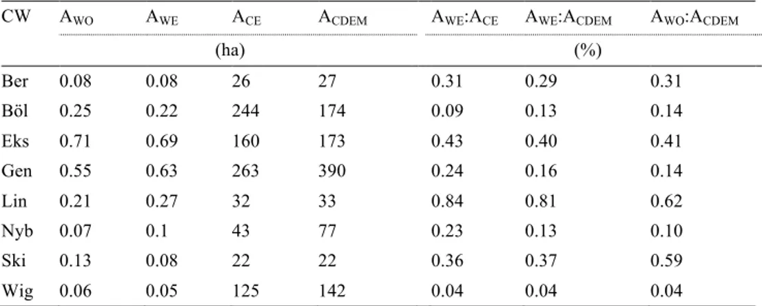
The different estimations of sizes of a CW and its associated catchment affects the AW:AC ratio. Three versions of the ratio were calculated (Table 3) (Appendix 2). AWE:ACE are the previously estimated ratios, AWE:ACDEM are the ratios using esti-mated CW areas and DEM catchments, and AWO:ACDEM are the ratios as they appear currently, using orthophoto determined CW areas and DEM delineated catchments. Estimated mean AWE:ACE was 0.32 % whilst AWO:ACDEM was on average 0.29 %. When looking at all 39 CWs, mean AW:AC and AWO:ACDEM were 0.65 and 0.41 % respectively, excluding Lif that did not have ACE and had AWO:ACDEM at 18 %.
Table 3. Wetland to catchment area ratios of 8 wetlands using previously estimated values only
(AWE:ACE), estimated wetland area and DEM determined catchments (AWE:ACDEM) and orthophoto
de-termined wetland areas and DEM dede-termined catchment (AWO:ACDEM).
CW AWO AWE ACE ACDEM AWE:ACE AWE:ACDEM AWO:ACDEM
(ha) (%) Ber 0.08 0.08 26 27 0.31 0.29 0.31 Böl 0.25 0.22 244 174 0.09 0.13 0.14 Eks 0.71 0.69 160 173 0.43 0.40 0.41 Gen 0.55 0.63 263 390 0.24 0.16 0.14 Lin 0.21 0.27 32 33 0.84 0.81 0.62 Nyb 0.07 0.1 43 77 0.23 0.13 0.10 Ski 0.13 0.08 22 22 0.36 0.37 0.59 Wig 0.06 0.05 125 142 0.04 0.04 0.04
3.1.2 Land use distribution
Only 22 CWs had available information on estimated land use distribution in the catchment areas, with an average of 54 % agricultural land. Land use analysis of DEM catchments using data from PLC-6 showed generally lower share arable land with a mean of only 37 % for the 22 catchments (paired t-test p=0.0002) (Figure 3). There was no significant correlation between size of catchment and percent differ-ence in agricultural land. Other than arable land, main categories of land use within DEM catchments were forest (22 %), open land (13 %) and pasture (7 %). The av-erage share of arable land including all 39 catchments was 45 % arable land, fol-lowed by 38 % forest, 11 % open land and 7 % pasture.
3.2 Phosphorus accumulation
Accumulated P from Kynkäänniemi (2014) was put in relation to new estimations of wetland and catchment factors. Correlations between modelled hydraulic loads, L:W, AW:AC, share arable land and DSMS clay content were studied. After a per-forming a PCA, multiple regressions were modelled to calculate the potential P ac-cumulation for the 39 CWs.
3.2.1 Annual versus extreme modelled hydraulic loads
All modelled HL were calculated using ACDEM and AWO initially, with the intention to predict P accumulation for the 31 new CWs using their current CW area and DEM determined catchments. However, AWE for the 8 CWs were true for the time P ac-cumulation was measured and therefore modelled HL calculated using AWE was also tested. The analysis showed a polynomial fit of yearly long-term average HL to give the strongest correlation with P accumulation (R2 = 0.84, p = 0.0045; equation 4).
y = 101.26932 + 0.568528M − 0.0042062 ∗ (M − 178.026); (4.)
Figure 3. Previously estimated agricultural land (%) versus agricultural land
in 22 DEM determined catchments using land use data from PLC-6 (Widén-Nilsson et al. 2016). Size of markers indicates relative size of DEM catch-ment. The line represents 1:1 relationship.
Agricultural land, DEM & PLC determined 0%
20% 40% 60% 80% 100%
DEM determined catchment (ha)
0% 20% 40% 60% 80% 100%
The 95th percentile of long term annual average was the 5th best fit (R2 = 0.82, p = 0.0062) (Appendix 3). All further analysis of HL was performed using ACDEM and AWO.
Using ACDEM and AWO for the 8 CWs, all different HL calculations were plotted against P accumulation (Kynkäänniemi 2014) and thereafter a line of best fit was calculated (Table 4). Polynomial (squared) line was shown to be the best fit. All 8 CWs were included (Kynkäänniemi (2014) excluded two small CWs with very high HL). As the fits were so similar, further analysis was only made on annual long-term average of HL (Equation 5), since this is potentially the most easily available data.
y = 122.30318 + 0.4628089 ∗ x − 0.0054018 ∗ (x − 171.729); (5.)
Table 4. Polynomial fit of 8 wetlands P accumulation and modelled hydraulic load (HL) using ACDEM
and AWO, and previously used data of short-term (2-3 years) average HL (Kynkäänniemi, 2014).
Mod-elled HL-data of mean, maximum and 95th percentile of monthly and annual average was obtained for
the time periods 1999-2017 (long-term), 1999-construction year and construction-2017 (CW life-time) from SMHIs water web (SMHI, 2019). One CW was constructed 1997 and thus not included in some time periods. Max HL and P accumulated is the vertex point of the polynomial fit.
HL
(m yr-1) Time period n R
2 P-value Max HL
(m yr-1) Max P acc (kg ha-1 yr-1)
monthly average 99-construction 7 0.965 0.0005* 214 238 annual average 99-construction 7 0.965 0.0005* 214 238 monthly average CW life-time 8 0.933 0.0005* 215 211 annual 95th% CW life-time 8 0.932 0.0005* 282 211 annual average CW life-time 8 0.932 0.0005* 214 211 monthly average long-term 8 0.931 0.0005* 215 211
annual 95th% long-term 8 0.931 0.0005* 281 210
annual average long-term 8 0.930 0.0006* 215 212
annual max long-term 8 0.930 0.0006* 303 208
annual max 99-construction 7 0.926 0.0025* 276 229
average* short-term 8 0.262 0.2018 196 176
* All eight wetlands were included in the polynomial fit.
A paired t-test of the 8 CWs previously determined HL and the modelled annual long-term average HL showed the mean difference to be 29 % but not statistically significant. There was a large variation between the modelled long-term average and the previously determined short-term average (Figure 4). Ski, Lin, Eks and Ber were similar comparing the two averages whilst Böl, Gen and Nyb differed with more than 100 m yr-1 between the short-term average and the modelled long-term HL average. In three cases (Ski, Eks and Ber) the short-term average HL exceeded the modelled long-term average and in Ski the short-term average HL was higher
than long-term maximum. Böl and Wig, the CWs with the highest HL, were ex-cluded in Kynkäänniemi’s (2014) line of regression.
The polynomial fit for accumulated P in relation to yearly long-term average HL (R2 = 0.93) has a vertex point of HL 215 m yr-1 (Figure 5). Note that the modelled HL is based on ACDEM and AWO, different from the CW and catchment areas used
Figure 5. Phosphorous accumulation determined by Kynkäänniemi (2014) in 8 wetlands in relation
to hydraulic load (HL) used by Kynkäänniemi (2014) (linear fit, R2 = 0.74, n = 6) and modelled
long-term average (polynomial fit R2 = 0.93, n = 8). Modelled HL is based on catchment areas
determined using DEM and wetland areas determined using orthophotos.
Accumulated P (kg ha-1 yr -1) 0 50 100 150 200 250 0 50 100 150 200 250 300 350 400 450 Hydraulic load (m yr-1)
Modelled long-term average, polynomial fit Kynkäänniemi (2014), linear fit
Ber Böl Eks Gen Lin Nyb Ski Wig
HL Modelled long-term average HL Kynkäänniemi (2014)
Figure 4. P accumulation in eight wetlands and hydraulic load (HL) as short-term average
used by Kynkäänniemi (2014) (circle), modelled long-term average (square) and long-term maximum (cross). Hydraulic load (m yr -1) 0 100 200 300 400 500 600 0 50 100 150 200 250 P accumulated (kg ha-1 yr -1)
Wig Ski Lin Eks Böl Ber Gen Nyb
Wetland
P accumulated HL Kynkäänniemi (2014) HL modelled long-term average HL modelled long-term max
by Kynkäänniemi (2014), as well as that the values for Wig and Böl that Kynkään-niemi (2014) excluded are not presented. Plotting modelled long-term maximum HL versus accumulated P showed a very similar pattern, only transposed towards higher HL. It did not describe the relationship to accumulated P better than the mod-elled average HL.
The distribution of the modelled long-term annual average tended towards lower HL (Figure 6). Fourteen of the CWs have HL lower than 50 m yr-1. The range of HL studied by Kynkäänniemi (2014) was approximately 20-120 m yr-1, excluding Böl and Wig. When calculating the modelled long-term annual average HL for the 39 wetlands, 15 were within this range (20-121 m yr-1). Including Böl and Wig, the previously studied range is approximately 20-400 m yr-1, where 32 of the modelled HL are within the range. Ten CWs had modelled HL in the range 145-255 m yr-1, around the vertex of the polynomial fit.
3.2.2 Wetland size in relation to catchments and wetland shape
Hydraulic load and the AW:AC ratio are generally negatively correlated, the smaller the ratio the larger the HL, since a larger catchment would drain into a relatively smaller wetland. For example, in Figure 6, the CW Ska had HL of 691 m yr-1 due to a very low AW:AC (0.03 %). Plotting long-term average HL versus AWO:ACDEM gave a log-transposed regression with R2 = 0.80 and p = 0.002. Of the three AW:AC (Table 3), only AWO:ACDEM, the ratio of the determined current areas in this study, showed significant correlation to accumulated P. The logarithmic function of P ac-cumulation and AWO:ACDEM, Wig excluded, gives R2 = 0.83; p = 0.003; also exclud-ing Böl gives R2 = 0.96; p = 0.0005 (Figure 7). There was no correlation between AWE:ACE and P accumulation (R2 = 0.2; p = 0.2), nor between AWE:ACD and accu-mulated P (R2 = 0.4; p = 0.07). For all three versions of the ratio, there appears to
Figure 6. Distribution of the modelled long-term average hydraulic loads
for 39 wetlands. Striped area shows the 8 previously studied, solid shows the 31 added wetlands.
Count 2 4 6 8 10 12 14 0 50 100 150 200 250 300 350 400 450 500 550 600 650
be a break point just under 0.1 % as both Wig (0.04 % in all ratios) and Böl (AWE:ACE 0.09 %) showed much lower P accumulation than Nyb (0.1 %).
The length to width ratio (L:W), orthophoto estimated, did not show any strong correlation but a positive trend could be seen in relation to P accumulation (R2 = 0.04; p = 0.3).
3.2.3 Soil texture and particle-size distribution on arable land
There was no statistically significant correlation between Kynkäänniemi’s (2014) accumulated P and share arable land estimated using PLC-6 data (R2 = 0.12, p = 0.39, n = 8). When studying estimations of soil particle-size distribution in relation to arable land (Share PLC-6 determined arable land*DSMS soil fraction) there were negative but not statistically significant trends between accumulated P and clay con-tent (R2 = 0.29; p = 0.12) and silt content (R2 = 0.23; p = 0.15) (Nyb excluded), (Figure 8). Sand content in relation to arable land showed no trend. Böl, Eks, Gen and Lin each had 1 % organic soils in the catchment, the others none. Regarding particle-size distribution, unrelated to the share of arable land, only silt showed a correlation with accumulated P (negative correlation R2 = 0.75; p =0.007). There was a positive trend between accumulated P and sand (Nyb excluded, R2 0.47; p = 0.052) and a negative trend between accumulated P and clay (Nyb excluded, R2 0.15; p = 0.21), but none of the trends were statistically significant.
There was no correlation between the distribution of soil textural classes within arable land and accumulated P except for loamy sand which had a positive correla-tion (Nyb excluded, R2 = 0.82; p = 0.003).
Figure 7. AWO:ACDEM in relation to accumulated phosphorus in the
8 wetlands. Dashed line R2 = 0.83; p = 0.0027 (excluding Wig). Solid line R2 = 0.96; p= 0.0005 (excluding Wig and Böl).
0 50 100 150 200 250 Accumulated P (kg ha-1 yr -1) Wig Nyb Böl Gen Ber Eks Ski Lin 0,0% 0,1% 0,2% 0,3% 0,4% 0,5% 0,6% 0,7% Aw:Ac
Modelled particle load to the CWs was tested using the model results from Djodjic & Markensten (2018). However, only weak trends could be seen between accumulated P and modelled particle load. Generally, the higher silt and clay con-tent, the more accumulated particles were modelled to enter the CW, and the more sand the less accumulated particles entered the CW.
3.3 Potential P retention
It has been shown that primarily modelled annual average HL and AW:AC affect P accumulation in a wetland, but there are also some trends between L:W and soil fractions. A principal component analysis (PCA) was made including the expected influencing factors (Figure 9). Based on the PCA, multiple regression analyses (MRA) were made using the factors HL, AWO:ACDEM, L:W, clay content from DSMS analysis and arable land determined using PLC-6 (Table 5). Including 5 factors showed a high statistical significance (R2 = 0.9985; p = 0.0011), however, it was possible to exclude both clay content and L:W and still show a statistical signifi-cance using the three factors HL, AW:AC and share arable land (R2 = 0.765; p= 0.0322). Excluding any other factor made the MRA not statistically significant.
Figure 8. Soil particle-size distribution of the arable land within the catchments of eight
wet-lands and their respective accumulated phosphorus. Horizontal lines show arable land (%) within the catchment.
Arble land and particle-size distribution (%)
0 20 40 60 80 100 0 50 100 150 200 250 Accumulated P (kg ha-1 yr -1)
Wig Ski Lin Eks Böl Ber Gen Nyb
Wetland Clay Silt Sand Organic Arable land P accumulated
Table 5. Multiple regression analysis (MRA) including five and three factors (n=8), explaining potential accumulated P (kg ha-1 yr-1).
5-factor MRA 3-factor MRA
Factor Estimate p-value Estimate p-value
Intercept 579.31236 0.0003 463.04137 0.0047
AWO:ACD (%) -190925.8 0.0004 -118152.7 0.0096
HL modelled long-term annual
average (m yr-1) -1.955426 0.0004 -1.325183 0.0134
Arable land (share) 733.94213 0.0006 366.50747 0.0383
L:W orthophoto -6.209997 0.0023
DSMS clay (%) 2.3678276 0.0039
R2 0.9985 0.765279
p-value 0.0011 0.0322
Figure 9. Principal components analysis showing how factors relate to P accumulated
(kg P ha-1 yr-1) and to each other.
-1,0 -0,5 0,0 0,5 1,0 Component 2 (25,7 %) AWO:ACDEM DSMS silt % DSMS clay % PLC arable share AWO P accumulated
HL long-term annual average
L:W ortho
ACDEM
-1,0 -0,5 0,0 0,5 1,0
Potential P accumulation was calculated for the 39 CWs using the equations from both MRAs as well as the polynomial fit of modelled long-term annual average HL, (Appendix 4). These three different methods of calculating potential P accumulation produced varying results (Figure 10). The 5-factor MRA showed both the highest and the lowest potential P accumulation (568 and -34744 m yr-1, respectively), with a wider range of potential P accumulation given the same modelled HL compared to the other two calculations. The threshold point of when HL starts to affect poten-tial P accumulation negatively appeared higher when using the polynomial fit, with the most potential P accumulation occurring in a CW with 211 m yr-1, compared to 184 m yr-1 for both MRAs.
Some CWs were calculated to have a negative potential P accumulation, i.e. net P release. For the polynomial fit, four CWs with modelled HL<16 or >690 m yr-1 showed negative potential P accumulation. For the 5-factor MRA calculations, 14 of the CWs showed net P release. Out of these, 10 had modelled HL <35 m yr-1, the other 4 had modelled HL ≥350 m yr-1. A
W:AC was ≤0.05 or >0.5, the other three factors had a high variation. For the 3-factor MRA, 15 of the CWs showed net P release, with the same parameter-ranges for HL and AW:AC as the 5-factor MRA, with a high variation of share arable land.
Figure 10. Potential phosphorus accumulation > -50 kg P ha-1 yr-1. Several CWs were calculated
to have negative P retention, most of which are not shown in this graph. Polynomial fit calculated 4 CWs to be negative, 5- and 3-factor multiple regression (MRA) equations calculated 14 and 15 CWs, respectively, to have a negative P accumulation.
Potential P accumulation (kg ha-1 yr
-1) 0 100 200 300 400 500 600 0 100 200 300 400
Hudraulic load, modelled long-term average (m yr-1)
Polynomial fit 5-factor MRA 3-factor MRA
4.1 Using different tools to estimate catchment areas
A systematic review has shown the P retention efficiency of a CW is highly affected by both P load and HL (Land et al. 2016). Therefore, it is essential that a CW is constructed to an optimal size and in a well selected location in relation to its catch-ment. To determine an efficient size of the wetland it is necessary to make accurate estimations of the catchment area to be able to reliably determine land use and par-ticle size distribution i.e. to better estimate P load and HL. There are different meth-ods of estimating catchment areas, giving varying results. This study has shown that using DEM to delineate catchment boundaries leads to 8 % larger areas compared to the currently most common method of using low resolution topography maps.
The share of arable land was often lower using ACDEM and PLC-6 data compared to previously estimated areas and land use distribution (Figure 3). As the DEM de-lineated catchments were larger than the originally estimated, and the share arable land lower, most of the areas added by DEM delineation were not arable land. Esti-mated areas of other land uses within ACE was mostly lacking, but as arable land stands for most of the P-load, with approximately 10 to 20 times higher area-specific loads compared to open land and forest (Nilsson et al. 2016), it would mean that a larger catchment area with less arable land gives a higher HL with a lower concen-tration of P. As P load has been proven positively correlated with area specific P retention (kg P per wetland and year) (Weisner et al. 2016), even though the differ-ence between the estimated and the DEM delineated catchment areas not always of arable land, they should not be disregarded as they will affect HL and thereby the potential P retention. Once the area of arable land is determined, the DSMS can be used to estimate particle-size distribution as also this can influence P load.
There are several sources of error when using DEM to delineate catchments. Information on tile drainage of arable land within the catchments was lacking in this
study and could affect the catchment areas, either by including or excluding artifi-cially drained fields. In some cases, it was possible to see on orthophotos if fields were drained at which point they were added or removed from the DEM catchment, but the uncertainty should be acknowledged.
As the efficiency of a CW is dependent on both P load and HL, it is of high importance to make accurate estimations of the catchment area. It is recommended to use DEM or another similarly detailed tool in combination with information on tile drainage to delineate the catchment and thereafter assess the potential P load and HL prior to construction.
4.2 Phosphorus accumulation and hydraulic load
Hydraulic load is significantly correlated to P accumulation and should be consid-ered when constructing a CW (Braskerud et al. 2005; Kynkäänniemi 2014). There is an interest in finding out the threshold point of when HL starts to negatively affect P accumulation to design more effective wetlands for nutrient retention. Kynkään-niemi (2014) found a strong positive correlation between HL <250 and P accumu-lation, and a detrimental effect on P accumulation when HL was 300 to 400 m yr-1. As the main P retention process in wetlands is sedimentation of particles, high flows indicated by high HL can wash out settled particles and thus affect the overall P retention. It was therefore expected to see a better explanation of the P accumulation using extreme HL compared to average HL. However, contrary to expectations, the ten best fits of modelled HL all show similarly significant relationships to P accu-mulation (Table 4). An explanation for the similarities could be that no extreme flows occurred during the time of P accumulation measurements, thus not reflecting the effects of extreme flows in this study. In other words, modelling HL as it has been calculated in this thesis, modelled maximum HL does not describe the pattern of the measured P accumulation better than the modelled annual average HL.
Kynkäänniemi (2014) excluded Wig and Böl, two small CWs with very high HL, exposing a linear fit between measured HL lower than 250 m yr-1 and accumu-lated P. In this thesis, all 8 CWs were included with a polynomial fit of the modelled annual long-term HL. Using a polynomial fit can allow for an estimation of where the optimal HL is in relation to P accumulation. It should be noted that the uncer-tainty is high with so few data points, particularly around the vertex. Especially so since Nyb had a high P accumulation due to ditch work during the time of sampling. However, assuming the HL calculations were reliable, and only regarding HL as influential to P accumulation, modelled long-term average HL can be used to predict P accumulation, with the threshold-point at 215 m yr-1 (Figure 5).
Data from SMHI’s S-HYPE model is easily accessible but may not always give an accurate estimation of HL in smaller catchments. Johannesson et al. (2015) found that modelled HL differed from measured HL values with 11-56 % when downscal-ing similar data for 7 of the 8 CWs. However, modelled HL in this study has been shown useful when estimating potential P retention, despite discrepancies between modelled data and measured values. Furthermore, the practicality of using modelled HL compared to measuring each time a wetland is to be constructed should not go unnoticed.
Wetlands are ever-changing ecosystems due to for instance processes of erosion and vegetation growth. Even though maintenance is supposed to retain the original size of the wetland, the estimated areas have in some cases been made even before construction. Occasionally, adjustments of the original plan are necessary during construction, meaning that the finished CW area differed slightly from the area orig-inally planned. Orthophotos can give an idea of the state of a CW, but they represent a snapshot of the specific time when the photograph was taken. AWO was used for analysis of the 8 CWs, and not the estimated areas. However, the modelled long-term average HL was also the best fit to accumulated P when using AWE, though the fit showed a maximum HL of 225 m yr-1, higher than when using AWO (215 m yr-1). Thus, even though there may be an error with using AWO instead of AWE, the error is both small and on the conservative side of the vertex point. Therefore, for this study orthophotos were considered sufficient in determining the current area of each CW as well as L:W. The difference in wetland size can however be decisive for different relations to other parameters, for example AW:AC. For higher accuracy in future studies, each CW could be visited and measured with proper instruments.
There is an uncertainty of estimates outside the measured range. When looking at modelled yearly average, 27 of the 39 wetlands were outside of the 8 CWs previ-ously studied HL range when excluding Böl and Wig. If all 8 CWs are included, only three CWs had modelled HL outside of the range. Some of the wetlands were calculated to have negative P retention, suggesting more P leaves the CW than what enters it, for example through internal erosion. However, most these CWs have modelled HL outside of the range, making the assumption that P loss is happening highly uncertain. Thus, the equations developed here should not be used outside the data range represented by the 8 measured CWs, and it is of utter importance to get additional measurements regarding P retention to further validate observed correla-tions.
Conclusively regarding HL and P accumulation, modelled long-term average is easily accessible, relatively stable, includes events of extreme flow, and can be used to describe potential P accumulation. There are however high uncertainties with only 8 data points as well as other factors other than HL that affects the overall P retention.
4.3 Potential phosphorus retention
Previous studies have found the assessed wetland and catchment factors included in this study to be correlated to P retention (Koskiaho et al. 2003; Senior 2011; Kyn-käänniemi 2014; Land et al. 2016). However, in this study only modelled HL and AW:AC were statistically significant when studying them as independent variables in relation to the 8 CWs P accumulation. The other factors, clay content, land use distribution and L:W showed trends, but were not significantly correlated to accu-mulated P. All five factors were however shown as statistically significant in the multiple regression analysis, with HL, AW:AC and share arable land as the most sig-nificant. All factors are dependent on AW and AC, which further highlights the im-portance of making accurate estimations of both catchment and CW areas.
The influence of clay content on P retention can be varying. Firstly, being the smallest particle, with a large specific surface, clay particles can bind large amounts of P. Secondly, clay particles can aggregate and act as larger particles, retaining P in the field. At the same time, aggregation in the soil can create macropores, facili-tating preferential flow and internal erosion, leading to a higher P and particle load (Jarvis 2007). Thirdly, smaller particles are at risk of not settling as fast as larger particles, potentially decreasing the P retention, whilst aggregated clay acting simi-lar to simi-larger particles can lead to a relatively high retention (Sveistrup et al. 2008). Johannesson et al. (2015), studying 7 of the 8 CWs (not Nyb), found a positive cor-relation between top soil clay content and clay within the sediment, with higher clay content in the sediment. Potentially, the reason this study did not show a more nu-anced result of clay content as an independent variable in relation to P accumulation is that clay content was averaged over the whole arable land within the catchments. Potentially, studying individual fields would generate a different result.
The multiple regression analysis using all 5 factors was statistically the most accurate but it is an over-parameterization which results in a sensitivity to variation of the parameters (Figure 10). The sensitivity could lead to over- or underestimation of potential P accumulation. Excluding clay content and L:W from the regression allowed for a more robust estimate considering the low population size (n = 8). With the 3-factor MRA, 12 CWs were calculated to have a potential P accumulation over 150 kg ha-1 yr-1. Amongst these there was a high variation of the parameters, sug-gesting they can compensate for one another, leading to it being difficult to deter-mine optimum values for each parameter.
There are uncertainties within the multiple regression. Firstly, this study is based on 8 CWs, a low number of observations for statistical analysis. Particularly CWs with parameter estimates outside the range of estimates for the 8 CWs should be treated with extreme caution. Secondly, there is the importance of wetland area, for