Early life economic shocks and child health outcomes

(1)

Department of Economics

Early Life Economic Shocks and Child Health Outcomes:

Evidence from Kenya

Douglas Kazibwe

Master´s thesis • 30 credits

Environmental Economics and Management - Master's Programme

Degree Project/SLU, Department of Economics • Part number 1198 • ISSN 1401-4084 Uppsala 2019

(2)

Early Life Economic Shocks and Child Health Outcomes: Evidence from Kenya

Douglas Kazibwe

Supervisor: Justice. T. Mensah, Swedish University of Agricultural Sciences, Department of Economics

Examiner: Rob Hart, Swedish University of Agricultural Sciences, Department of Economics

Credits: 30 hec Level: A2E

Course title: Master thesis in Economics Course code: EX0905

Programme/education: Environmental Economics and Management - Master's Programme Faculty: Faculty of Natural Resources and Agricultural Sciences

Course coordinating department: Department of Economics Place of publication: Uppsala

Year of publication: 2019

Title of series:_{Degree Project/SLU, Department of Economics} No: 1198

ISSN: 1401-4084

Online publication: https://stud.epsilon.slu.se

Keywords: Height-For-Age, Under-Five Mortality, Early Life, Commodity Prices, Human Capital, Kenya

Swedish University of Agricultural Sciences

Faculty of Natural Resources and Agricultural Sciences Department of Economics

(3)

Abstract

This paper examines the relationship between commodity price shocks experienced in the early period of life and child health outcomes. The study uses a nationally representative household survey data from the Demographic and Health Surveys in Kenya matched with a time series of real producer prices of tea in estimating the effect of price shock on child health outcomes. The identification strategy of the paper relies on exogenous variations in the real producer price of tea and timing of child birth. The findings show that household income shocks induced by variations in tea prices are key drivers of child health outcomes. A one percentage increase in tea price in the early life stage improves child nutrition with a 32.67 standard deviation increase in height-for-age Z scores and reduces under-five mortality rate by 1.74 percentage points among children born in tea producing zones relative to those born in non-tea growing zones in Kenya.

These study findings have much policy relevance to African economies where a considerable share of the population depends on the agriculture sector as a source of livelihood, and directly suffers from export commodity price fluctuations. Changes in the commodity price of exports are a constraint that weigh on agricultural households’ ability to make necessary investment in children thus impacting health and human capital formation.

(4)

List of Abbreviations

AEZ Agro-Ecological Zone

DHS Demographic and Household Surveys

FAO Food and Agriculture Organisation of the United Nations FAOSTAT Statistics Division of FAO

GDP Gross Domestic Product

ha Hectare

HAZ Height-for-age Z-scores

KES Kenya Shillings

Kg ha-1 _{Kilogram per Hectare, per annum}

KDHS Kenya Demographic and Household Survey KMD Kenya Meteorological Department

KNBS Kenya National Bureau of Statistics KTDA Kenya Tea Development Agency Ltd KTGA Kenya Tea Growers Association

TBK Tea Board of Kenya

TRI Tea Research Institute U5MR Under-Five Mortality Rate

(6)

1. Introduction

Agriculture continues to be one of the most important sectors of the Kenyan economy, contributing substantially to employment and trade. It accounts for 32.6% of Kenya’s total GDP1_{(KNBS, 2017). Like in many Sub-Saharan African countries, most of Kenya’s labour} force is currently employed in the agricultural sector2_{. This makes agriculture a vital source of} employment for the country, most especially in rural areas where over 70% of the population depend on it for their livelihoods in the form of subsistence farming, cash crop production or as hired farm labour.

Agriculture is an activity mired in risk and uncertainty. It is predominantly rainfed and highly dependent on natural factors, thus, making yields sensitive to weather changes such as drought. Changes in policies and regulations also affect agricultural production and are risks that are usually manifested as constraints on production. For example, regulations on use of herbicides and fertilizers, increase costs of production; income tax or credit policies affect returns on output; while a foreign country’s decision to reduce imports of a certain crop may affect its price. As far as a farmer is concerned, tea prices are a non-controllable variable and solely determined at auctions (Baffes, 2005). Markets are complex and involve both domestic and international dimensions. For instance, tea producer returns in Kenya may be affected by events in other parts of the world that directly or indirectly influence world tea prices. These exogenous price variations create income volatility for the farmers, thus, affecting a farming household’s intertemporal budget.

In presence of risk and uncertainty, households cannot achieve optimal consumption streams overtime as farmers are faced with restricted coping mechanisms. At the local level, available informal risk-sharing mechanisms are narrow due to the nature of shocks to agriculture. For example, shocks such as pests or vagaries of weather tend to affect most people within a given geographical area. On the other hand, formal mechanisms such as agricultural credit or insurance schemes are limited (Kibaara, 2006; Kerer, 2013; Di Marcantonio & Kayitakire, 2017). This curtails consumption smoothing channels available and as a result, farmers cannot adapt and mitigate against aggregate shocks such as drought or a fall in commodity prices to protect their consumption and make much needed child investments. Therefore, income volatility, and constraints on saving and borrowing will ultimately negate a household’s ability

1_{Gross Domestic Product}

2_{As of 2017, employment in Kenya’s agricultural sector was 37.95% of total employment}

(7)

to smoothen consumption and pay for child-human capital investments over states of nature and across time.

Investment in children and human capital development are critical in a nation’s pursuit of economic growth and development. Nutritional status of children and under-five mortality rate are among the core indicators of sustainable development (United Nations, 2007, p 11), with which national governments used to measure progress on the Millennium Development Goals3 (MDGs). Adequate nutrition is critical to children’s growth, and development and it is one of the prerequisites for national development. In Kenya, there’s been an overall improvement in child nutritional status, with stunting declining from 38 percent in 1998 to 26 percent in 2014 (Kenya National Bureau of Statistics et al., 2015). However, child malnutrition remains a vital contributor to child morbidity and mortality as it leaves children susceptible to infectious diseases. Kenya’s under-five mortality rate has declined, from 98 deaths per thousand live births in 1990 to 52 deaths per thousand live births in 2014 (ibid.). Nevertheless, the rate is still below the minimum MDGs target of reducing under-five mortality by a two-thirds (Kimani-Murage et al., 2014; Keats et al., 2018). Therefore, more analytical studies on how best to implement national strategies/interventions to reduce child malnutrition and mortality are needed and this can be best achieved by examining household income, consumption and investment patterns. Understanding the impact of aggregate shocks on child nutritional status and mortality can enable policy makers set and achieve sustainable development targets. There are a reasonable number of studies that consider how aggregate shocks such as those caused by macroeconomic crises, shocks on production or policy reforms influence child human capital investments in developing countries. Using econometric methods, researchers have utilized natural experiments based on macroeconomic crises (Baird et al., 2011; Pongou et al., 2006; Paxson & Schady, 2005) to show the relationship between economic downturns and child health outcomes. Others have focused on agricultural incomes, scrutinizing shocks on agricultural production (Jensen, 2000; Hoddinott & Kinsey, 2001; Yamano et al., 2005; Alderman et al., 2006) or commodity price fluctuations (Maluccio, 2005; Miller & Urdinola, 2010; Cogneau & Jedwab, 2012; Adhvaryu et al., 2018). This paper contributes to the latter

3_{The Millennium Development Goals were derived from the United Nations Millennium}

Declaration adopted by 189 nations in 2000. Most of the goals and targets were set to be achieved by 2015 based on the global situation during the 1990s. 1990 is the baseline year

for assessment on each nation’s progress. In 2015, the MDGs were replaced with Sustainable Development Goals (SDGs) ( https://sustainabledevelopment.un.org/topics/sustainabledevelopmentgoals)

(8)

strand of analysis, investigating the relationship between changes in real producer prices of tea and child health outcomes in Kenya.

Currently, only a small proportion of the literature available on early life circumstances is focused on the impact of aggregate economic shocks emanating from commodity price variations. This is despite the evidence that many developing countries are highly vulnerable to variations in commodity prices (Deaton, 1999) owing to a large percentage of their rural population being dependent on agricultural production as a source of livelihood. In this study, I aim to fill this gap by investigating the following question: how does tea price shock at time of birth affect child nutritional status and mortality within the tea growing zones of Kenya? Evidence suggests that aggregate shocks experienced during early life stage have a tremendous impact on child nutritional status, mortality, and schooling (Ferreira & Schady, 2009). To examine this relationship, I use econometric analysis on a nationally representative dataset for children under five years from the Kenya Demographic and Household Surveys (KDHS). I combine KDHS data with a time series of real producer prices of tea, coupled with Agro-Ecological Zone data (AEZ) to map out tea growing zones. I intend to exploit variations in early life circumstances induced by changes in the real producer price of tea to answer the research question. As a major economic activity in the tea growing zones, tea price revenue is treated as the primary determinant of household income. Furthermore, it should be noted that the variation in tea prices has a knock-on effect on non-tea farming household incomes in tea growing areas. This is because, the tea industry in Kenya has an intricate value chain which includes tea growing, processing, and trade. There are different stakeholders along the value chain, whom among others include farmers, green leaf collectors, transporters, tea processing (blending and packing) factory workers, warehousing, traders/auctioneers and customs officials (Elbehri et al., 2015, p 22). Therefore, exposure to price variations cannot be limited to tea farmers.

The ambit of this research is limited to the country of Kenya, for the time-period between 1998 to 2014. The necessary data points needed for this analysis are readily available for the given time. The study aims to expound on the nexus between changes in tea producer prices and child nutritional status, and under-five mortality rate in Kenya.

The remainder of this thesis is organized as follows. Chapter 2 presents the literature review, which covers empirical studies on early-life-shocks, child nutritional status and mortality. Chapter 3 expounds on tea production in Kenya, with discourse on the genesis of tea growing

(9)

in Kenya, it’s cultivation, and the value chain. This enables the reader to understand the importance of the tea sub-sector to the Kenyan economy. Chapter 4 introduces the conceptual framework. Chapter 5 presents the identification strategy used in the analysis of the research question. It discusses the econometric model specifications. Chapter 6 presents data sources; selected variables are introduced and details on each are explained further. An overview of estimation results from the econometric analysis and discussion of these results is presented in chapter 7. Chapter 8 presents the conclusion and recommendations.

(10)

2. Literature Review

Current empirical evidence on effects of aggregate shocks on child nutritional status and mortality in the developing world and particularly in Africa suggests outcomes are procyclical i.e., child mortality and malnutrition rise during periods of aggregate shock (Jensen, 2000 for Ivory Coast; Yamano et al., 2005 for Ethiopia ; Alderman, 2006 for Zimbabwe; Pongou et al., 2006 for Cameroon; Cogneau & Jedwab, 2012 for Ivory Coast). For middle-income nations of South America, health outcomes are mixed i.e. procyclical (Maluccio, 2005) and counter-cyclical (Miller & Urdinola, 2010). Results from developing nations contrast those of developed nations like the United States of America (Dehejia & Lleras-Muney, 2004), where health outcomes are generally counter-cyclical. Below, I review literature on the impacts of aggregate shocks on child nutritional status and mortality in African and Latin American countries.

2.1. Nutritional Status

Cogneau & Jedwab (2012) investigate the impact of sharp fall in the administered producer price of cocoa in Ivory Coast during 1990, on investments among children of cocoa producing households. They analyse the extent of the impact of this economic shock on child investments among cocoa producers and make comparisons with children of non-cocoa producing households. Data before the crisis (1986-88) and after the crisis (1993) is used for the comparison. To achieve this, a difference-in-differences within-village strategy is employed to identify the causal effect of household income on child outcomes between children living in cocoa producing households (treatment group), and those in living in other agricultural households (control group) within the same village. The main regression model uses either district-year or village-year fixed effects to control for all factors common to all children living in the same area within the same year. Four outcomes of interest are examined i.e., school enrolment, labour, height-for-age and morbidity and results show a strong causal effect across all four. Height-for-age declined significantly with a loss between 0.25 and 0.62 international standard deviations in height-for-age Z scores among children aged between 2 to 4 years old. There was increased morbidity by 3 to 4 percentage points among children from cocoa producing households in comparison to their counterparts in non-cocoa producing households. Furthermore, results on gender show that girls were more affected than boys, a result which contrasts findings by Pongou et al., (2006) for Cameroon. It should be noted that, Cogneau and Jedwab’s analysis is limited as they exploit a negative income shock in the form of a reduction in price of cocoa in 1990, an event which occurred over a short period.

(11)

For Nicaragua, Maluccio, (2005) analyses the impact of a sudden reduction in the price of coffee between 2000-02 on child health status in coffee growing areas. His study is similar to Cogneau & Jedwab (2012) in exploiting a negative income shock i.e. fall in prices. He used data collected for the analysis of the impact of a conditional cash transfer program, the Red de Protección Social (RPS) that was implemented during this economic downturn. In the program, households were randomly assigned to treatment and control groups. Results in the analysis show that per capita consumption for households in the control group (those not assigned to the cash transfer program) fell on average by 10%. The reduction in consumption was larger in coffee growing areas by approximately 27%. Contemporaneous with these reductions in household per capita expenditure, height-for-age z scores of children aged 6 to 48 months declined by 0.148 percentage points. This result matches the findings of Cogneau & Jedwab (2012). However, one major weakness of Maluccio’s analysis is that the data used was not nationally representative, since it only covered households in selected rural areas.

Pongou et al., (2006) utilizes pooled cross-sectional data from two Demographic and Health Surveys (DHS) conducted in 1991 and 1998 to study the impacts of macroeconomic crises and policies with the aid of ordinary least-squares regression. They show that a macroeconomic decline in Cameroon is equivalent to an increase in weight-for-age Z scores (a composite indicator of acute and/or chronic malnutrition) by 9 percentage points for boys and 3 percentage points for girls. Children of uneducated mothers are more likely than those of primary schooling to become malnourished. Children of mothers with secondary education fair better than those with primary schooling. This shows that mother’s level of education has significant impact on child nutrition. Malnutrition is also found to be more pronounced among children in rural based households than those in urban areas, and among households with fewer assets. These results on maternal education and gender of child echo the findings of Kabubo-Mariara et al., (2009) in their analysis of child nutritional status determinants in Kenya. In the analysis, they find that boys suffer more malnutrition than girls and children of multiple births are more likely to be malnourished than singletons. It is also observed that maternal education and household wealth are vital determinants of child nutritional status in Kenya. These results (i.e. Pongou et al., 2006; Kabubo-Mariara et al., 2009) on gender of child contrasts the findings made by Cogneau & Jedwab (2012).

In Ivory Coast, Jensen (2000) uses a difference in difference method to show how exposure to drought affected nutrition before and after the shock. Results show that malnutrition increased for all groups but there is a large increase for those in shock areas. Exposure to drought is

(12)

associated with more than two standard deviations below the reference median. For Zimbabwe, Hoddinott & Kinsey (2001) examine the impact of the 1994/95 drought on child health in rural areas using a panel data set. They find that children aged 12 to 24 months affected by the drought lose 1.5 ‐ 2 cm of growth in the aftermath of drought. Four years after the drought, these children remained shorter than identically aged children who didn’t experience the drought. Similarly, using three nationally representative surveys conducted during 1995–96 in Ethiopia, Yamano et al., (2005) finds that a 10-percentage point increase in the proportion of damaged plot areas within a community corresponds to a reduction in child growth by 0.12 cm over a six-month period. All these studies explore the effects of drought on child investments during early childhood stages and conclude that a drought shock leads to a negative change in child nutritional status.

2.2. Child Mortality

Paxson & Schady (2005) examine the effects of economic crisis on child health in Peru during the late 1980s using DHS data. Their results show that a spike in infant mortality coincides with economic crisis; there’s an increase in infant mortality from about 50 deaths per 1000 live births to 75 deaths. They estimate a 2.5 percentage point increase in infant mortality rate for children born during the late 1980s, which implies that approximately 17,000 more children died than would have occurred in the absence of the crisis. Infant mortality peaked in 1990 when real wages were at their lowest. Paxson and Schady indicate that the crisis could have worked through two channels. First, the deterioration of public health services which led to a reduction in the use of health services. Second, it led to a decline in household expenditures on inputs to child health, including nutrition or medical care for both mothers and children. With a reduction in household income and consumption, it is assumed that expenditure on inputs vital for determining child health would have to be scaled back by households to meet its optimal budget allocation. However, due to lack of information on household expenditure, this channel is not fully examined. In the analysis, infant mortality is found to be higher among children of less educated mothers. This result matches the findings by Baird et al., (2011), who concludes that infant mortality is larger during economic crisis among children of less educated women than those with higher educated mothers.

Baird et al., (2011) used DHS data consisting of 1.7 million births from 59 developing countries to investigate whether short-term fluctuations in aggregate income affect infant mortality. With an unusually large data set, they construct country-specific infant mortality rate series, and merge it with data on real GDP per capita, adjusting it for differences across countries in

(13)

purchasing power parity. In the regression analysis, they account for country-specific trends in the infant mortality rates and GDP per capita in the pooled survey data. Results indicate that income shocks have large negative effects on infant mortality viz a 1% decrease in per capita GDP is associated with a 0.24 to 0.40 percentage increase in infant mortality per 1,000 live births.

In the analysis, they also include mother fixed effects and birth-specific characteristics in their regression model and find that the coefficients estimated are like those without fixed effects. This makes it clear that change in composition of women doesn’t account for the association between infant mortality and GDP per capita observed in the data. Furthermore, they include timing of shocks in the model using lagged terms and conclude that that economic conditions during months shortly before and immediately after birth have a sizeable effect on the probability that a child survives. The transmission mechanism from aggregate economic shock to infant mortality can be best explained in this process. Results further show that mortality among infants born to less educated mothers is almost twice as high when compared to that of children born to mothers with higher education; children born to young mothers (15-19) and older mothers (35-39) are more likely to die than those born to prime mothers (20–34); that high-parity births (higher birth order) are more likely to die than low-parity births; and children born to mothers in rural areas are more likely to die than those born to mothers in urban areas. The results on mother’s age, education and child birth order are analogous to findings by Horton (1988) and Finlay et al., (2011).

In their investigation of how cocoa price variations experienced during early life stage affect adult mental health, Adhvaryu et al., (2018) also considers the magnitude at which cocoa price shocks affect infant mortality in Ghana’s cocoa producing regions. Using DHS birth recode, they test for selective mortality in the data set. The econometric model specification used, controls for both maternal and paternal characteristics, and considers region-specific-time trends, and region fixed effects. Results indicate that increases in cocoa prices predict higher mortality. This result is similar to the main findings in the analysis of coffee price fluctuations in Columbia by Miller & Urdinola (2010) who conclude that infant mortality increases when there are positive price shocks.

For Colombia, Miller & Urdinola (2010) analyse three different coffee price shocks on infant mortality in coffee growing regions of Colombia. They examined how child survival in Colombia responds to fluctuations in world Arabica coffee prices. The supply shocks that led

(14)

to sudden changes in Colombia’s internal coffee prices were because of the 1975 frost that destroyed Brazil’s coffee harvests; a drought in Brazil in 1985, and the collapse of the International Coffee Agreement between 19989-1990 that caused abandonment of export quotas by 1991. Miller and Urdinola use population census and DHS data to analyse changes among cohorts born in the shock years or only those conceived prior to the shocks. With this restriction, it is assumed that price shocks do not affect mortality among the older children. They employ a cohort study framework using the difference-in-differences estimation strategy to exploit the differences between coffee growing and non-coffee growing areas of Colombia. Results show that infant mortality increases when there are positive price shocks (higher incomes in coffee growing areas) and decreases with negative price shocks.

In summary, the reviewed literature paints a clear picture of how aggregate shocks have an impact on child health outcomes. In the developing world, child mortality increases during economic crises and decreases during economic expansion. This contrasts with findings from the developed countries and richer middle- income countries (Dehejia & Lleras-Muney, 2004; Ferreira & Schady, 2009) which show mortality decreasing during recession. Child nutritional status is also found to be decreasing during periods of economic crises, with an overall decline in height-for-age Z scores.

(15)

3. Tea Production in Kenya

Tea (Camellia sinensis) belongs to the family Theaceae (Camelliaceae). The genus Camellia developed in Asia centred around the Himalayan mountains and it was introduced to Kenya by the British settler, G.W.L. Caine in 1903 (Kagira et al., 2012). Tea is grown in volcanic soils consisting of Nitisols, andosols, cambisols and acrisols, with a soil pH between 4.5 -5.8. Tea growth requires mean annual temperature range between 13o_{C - 23.5}o_{C, annual rainfall ranging} between 1200mm -1400mm per annum (Carr, 1972), with alternating long sunny days. At altitudes of 1500 -2700m above sea level, the Kenyan highlands located on both the eastern and western sides of Gregory Rift (eastern branch of the Eastern Africa Rift) are particularly well-suited for tea cultivation. Tea is grown in 5 out of the 8 provinces of Kenya, with Rift Valley and Central provinces accounting for over 71% of total national output. Tea is also cultivated in Nyanza, Eastern and Western provinces of Kenya.

Cultivation is carried out on both smallholder farms and large tea estates. Smallholder farms account for 62% of Kenya’s total tea production, with farm size varying between 0.5 and 3.5ha. Smallholder farmers are suppliers and shareholders of tea processing factories owned by Kenya Tea Development Agency Ltd (KTDA), an agency representing smallholder tea farmers. KTDA factories process tea for auction sale as well as package and market it for local consumption. On the other hand, large tea estates are organized under the Kenya Tea Growers Association Ltd (KTGA) and account for the remaining 38% output4_{. These are mainly owned} by large multinational corporations such as James Finlay, Unilever and Cargill, and are a source of employment to the local population. It is estimated that the tea sector is the largest private employer in the private sector, with over 5 million Kenyans earning their livelihoods from the sector - a figure that consist of about 12% of the total population (Elbehri et al., 2015, p 18). Due to conducive weather conditions and tea research efforts by the Tea Research Institute (TRI), average yields have increased threefold from 711.9 Kg ha-1 _{in 1961 to 2192.6 Kg ha}-1 _in 2014. Overall production has increased making Kenya the third largest producer of tea as well as the number one exporter of black tea in the world5_.

Labour, tea cultivar type and fertilizers used are the three most important factors that greatly impact tea output and production costs. Labour in the tea sector falls into three categories; family labour on smallholder farms, seasonal and day laborers who live near farms and

4_{Refer to:}_{http://www.ethicalteapartnership.org/wp-content/uploads/ETP-Supporting-Smallholders-Part-1.pdf} 5_{Refer to:}_{https://inttea.com/}_{(2015 International Tea committee statistics report)}

(16)

plantations. Production requires considerable non-harvest maintenance which includes pruning, weeding, fertilizing and tea planting. In Kenya, tea is harvested all year round, following a 7-14-day interval schedule depending on the growth of tender shoots (Owuor et al., 2000). Bushes are plucked either by hand or machinery (in-case of large plantations), whereby the upper 2-3 leaves and bud are harvested. Farmers deliver their harvest to tea buying centres, where it is collected and delivered to processing facilities immediately to maximize tea quality (Elbehri et al., 2015, p 23). At the factory, leaves are withered to remove excess water and allowed to oxidize. Steel roller machines are then used to cut the leaves into small particles and then left to ferment for between 70-100 minutes. After fermentation, the tea is dried to remove excess moisture and then graded and forwarded to brokers at the Mombasa tea auction6_{. At auction, brokers set the value of tea according to the market. Samples with} accompanying information such as quality grade and tea farms are forwarded to participating companies for evaluation and bidding on a weekly basis.

6_{The auction is managed by the East Africa Tea Trade Association, which brings together the producers,}

(17)

4. Conceptual Framework

The conceptual framework for child health outcomes draws on the model by Ferreira & Schady (2009) who postulates a production function for child health with three main arguments, namely: private expenditures on promoting goods; private allocation of time to health-promoting activities, and public expenditures on health care. Note that, there may be other arguments in this production function but only the three aforementioned are considered in the framework proposed by Ferreira & Schady (2009). They find that these three arguments have a positive contribution to health outcomes but with decreasing marginal productivity.

In this analysis, I focus on the marginal productivity of private expenditures on health-promoting goods to shed light on the mechanism through which tea price shock affects child health outcomes in Kenya. Assuming tea price shock has no effect on the other two arguments, then the primary channel of impact on child health investments will be on the consumption side of health-promoting goods. These include: nutritious foods, clean water, vaccination, prenatal and postnatal care, mosquito nets, etc.

Health promoting goods are normal goods and are a part of the overall household consumption basket. A household will maximize utility subject to intertemporal budget constraints due to income variations emanating from tea price shock. If tea price shock increases household income, then the consumption of child health promoting goods will be strengthened thus having a positive impact on child health outcomes. When real producer prices are high, children born into households located in tea growing zones will get more resources allocated to them due to high returns from tea production. Increases in household income emanating from high price of tea leads to an increase in the amount of resource available to households within tea growing zones for allocation to members. More resources available for allocation translates into increased consumption of child health promoting goods such as increased vaccination doses, pre and post-natal medical visits, increase in duration of breastfeeding, etc. I expect these outcomes for Kenya to be procyclical in nature.

(18)

5. Empirical Strategy

5.1. Identification Strategy

To identify the causal impact of economic shocks on child health outcomes in Kenya, I exploit exogenous variations in tea prices and variations in the time of birth. With the exogeneity of tea prices, it should be noted that tea farmers at the local level cannot influence tea prices. As mentioned earlier on, tea prices are determined and set at the tea auction in Mombasa by brokers and as such local farmers do not determine how tea prices are set.

Furthermore, the timing of birth is exogenous to local changes in real producer price of tea. Prices used here are not average prices over the entire period but rather the specific producer price of tea at the time of birth. Conceptually, if tea farmers had some form of control over price setting, it would be difficult for them to strategically influence prices at the time when their children are most likely to be born. For these reasons, I argue that variations in tea prices and variations in the time of birth are plausibly exogenous to local economies.

The intuition used here is that households in tea growing zones experience changes in real producer price of tea as income shocks whereas households in non-tea growing zones are unaffected by these variations. Based on the use of real producer prices of tea7_{and the overall} contribution of the tea sub-sector to the total GDP of Kenya, it must be argued that spill over effects at household level in non-tea growing zones are limited and thus considered not to have repercussions on the identification strategy used.

Nevertheless, it must be stressed that the effect of tea price shock on child health status being estimated in this paper can be considered as an intent-to-treat (ITT) rather than the average treatment effect (ATE). This is because, the data used here identifies households based on whether they live in tea growing zones or not, rather than whether these households are tea growing or otherwise.

7_{Average prices of tea from auctions are not used here as a measure of an exogenous determinant of household}

income in tea growing zones. These prices may not reflect true farm gate prices faced by households in tea growing zones. Tea producer prices used are extracted from FAOSTAT’s Agricultural Producer Prices database.

(19)

5.2. Specifications

5.2.1. Child Height for Age

Using a pooled cross-sectional data set from Kenya, I analyse the effects of tea price shock in the year of birth on child health outcome. Child nutritional status is examined using the height-for-age Z scores (HAZ), which reports the difference between the child's height and the median height of a reference population of the same age and sex, expressed in units equal to one standard deviation of the reference population's distribution. HAZ between -2 and -3 is used to represent moderate chronic malnutrition, and below -3 to represent severe chronic malnutrition. I estimate the following equation below as the main specification:

𝐻_"#$ = 𝛼 + 𝛽 ln(𝑇𝑒𝑎𝑃𝑟𝑖𝑐𝑒_$) × 𝑇𝑒𝑎𝑃𝑟𝑜𝑑𝑢𝑐𝑒𝑟_#+ 𝛾𝑋_"#$+ 𝛿_#+ 𝜃_$+ 𝜖_"#$ (1) For each child 𝑖 observed in zone 𝑟 at time 𝑡, 𝐻"#$ is the outcome of interest (height-for-age Z

score8_{). 𝛼 is the intercept and 𝛽 is the coefficient of interest, 𝑇𝑒𝑎𝑃𝑟𝑖𝑐𝑒}

$ is the real producer

price of tea in year 𝑡. In the data section below, source and calculation of the real producer price of tea is described. 𝑇𝑒𝑎𝑃𝑟𝑜𝑑𝑢𝑐𝑒𝑟# is an indicator variable equal to 1 if tea is produced in

zone 𝑟 and 0 otherwise. The variable ln(𝑇𝑒𝑎𝑃𝑟𝑖𝑐𝑒_$) × 𝑇𝑒𝑎𝑃𝑟𝑜𝑑𝑢𝑐𝑒𝑟# shows the interaction

between log real producer prices of tea and the indicator for whether tea is produced in zone 𝑟. This interaction variable is referred to as the Price Shock, and I anticipate that a positive price shock results into a positive 𝛽 estimate which represents a positive change in mean height-for-age z-scores. It should be noted that 𝛽 estimate can be considered as an ITT estimate as opposed to the ATE estimate.

The term 𝑋"#$ is a set of vector controls and these include; parental characteristics (mother’s

level of education, and dummy variables for whether father and mother are employed in agriculture or not, mother’s age), household characteristics (rural or urban place of residence, household wealth and sex of household head) and child characteristics (sex of child and child birth order number). Interactions between the price shock variable and parental occupation are added. I also incorporate dummies for religion and ethnicity. The preferred baseline fixed-effects specifications also include; 𝛿# as a vector for zone of birth fixed effects and 𝜃$ for year

8_{Note that results for HAZ scores are an anthropometry measure expressed in reference standard deviation}

(20)

of birth fixed effects. Year of birth fixed effects are included to absorb unobserved differences across the years when children are born, zone of birth fixed effects controls for unobserved differences between Agro-Ecological Zones9_{(AEZ) that may affect health outcome. I include} survey year fixed effect to account for time varying factors across the survey years. 𝜖"#$ is the

error term. Standard errors are clustered at the level of survey clusters to avoid overoptimistic inference.

5.2.2. Under Five Mortality

DHS birth and women recodes are used to investigate the effect of tea price shock on child mortality, tea prices are exogenous to local changes in child mortality. The main specification used to capture the effect is as follows:

𝑀𝑜𝑟𝑡𝑎𝑙𝑖𝑡𝑦_"#$ = 𝛼 + 𝛽 ln(𝑇𝑒𝑎𝑃𝑟𝑖𝑐𝑒_$) × 𝑇𝑒𝑎𝑃𝑟𝑜𝑑𝑢𝑐𝑒𝑟#+ 𝛾𝑋"#$+ 𝛿#+ 𝜃$+ 𝜖"#$ (2)

where the outcome 𝑀𝑜𝑟𝑡𝑎𝑙𝑖𝑡𝑦_"#$ is an indicator that takes the value 1 if a child 𝑖, born at time 𝑡 and whose mother resides in zone 𝑟 died within the first five years of life and 0 otherwise (detailed explanation of variable in subsection 6.2). 𝛼 is the intercept; 𝛽 is the ITT estimate showing the impact of tea price shock on under-five mortality rate, here 𝑇𝑒𝑎𝑃𝑟𝑖𝑐𝑒_$ is the real producer price of tea in year 𝑡 and 𝑇𝑒𝑎𝑃𝑟𝑜𝑑𝑢𝑐𝑒𝑟_# is an indicator variable equal to one if tea is produced in zone 𝑟 and 0 otherwise. ln(𝑇𝑒𝑎𝑃𝑟𝑖𝑐𝑒$) × 𝑇𝑒𝑎𝑃𝑟𝑜𝑑𝑢𝑐𝑒𝑟# represents the tea price

shock variable measured in the child’s year of birth. The regression controls for 𝛿_# as a vector for zone of birth fixed effects and 𝜃_$ for year of birth fixed effects, and a vector of maternal and birth controls 𝑋"#$. As described in section 6.2 below, child birth and death are calculated

based on retrospective questions asked of mothers between ages 15-49 at the time of the survey and this limits the number of variables that can be included in (2). Maternal controls include mother’s age, age squared, education level, binary indicator for place of residence (rural/urban), dummies for both religion and ethnicity. Birth controls are child birth order, multiple birth and gender of child. 𝜖_"#$ is the error term. Standard errors are clustered at survey cluster levels to correct for autocorrelation.

In the baseline specifications above (equations 1 and 2), an additional control 𝜏_E$#FGE is added to each equation to allow for zone of birth specific time-trends. These are included to absorb extraneous variations overtime in the dependent variable at the zone of birth level in the new

9_{FAO (1996). Agro-ecological Zoning Guidelines. FAO Soils Bulletin 73.}

(21)

specifications. Note that, linkages between climate variations and change in prices of agricultural products exist. Fluctuations in rainfall received and changes in temperature influence agricultural output in-terms of quality and quantity. This in turn affects price and revenue received by households. Climate variations also do have a direct effect on the health of household members. These climatic factors indeed vary across AEZs, but this poses no problem to the preferred specifications as I control for unobserved differences between AEZs using zone of birth fixed effects. Policy changes or other unobserved factors changing annually are controlled for using birth year or survey year fixed effects and zone- specific time trends. This makes for more rigorous specifications to be adopted and are preferred to the baseline models (1) and (2).

Additionally, to investigate parental occupation effect on child health outcomes. I introduce the interaction term between Tea Price Shock and Agricultural parent (i.e. father and mother) dummy variables, where it is 1 for parents identified as agricultural workers and 0 otherwise. This enables me to use the same sample to estimate the magnitude of the price shock based on its interaction with parent’s occupation. The interaction terms are included in the preferred model specifications with birth specific time-trends.

(22)

6. Data

6.1. Tea Prices

The source of data for the tea producer prices and the Consumer Price Index (CPI) is FAOSTAT10_{and the World Bank}11_{respectively. I calculate real producer prices for tea using} the following:

𝑃_$# _{= H}IJKLMN IJKL O ∗ 𝑃"

Where 𝑃" is the nominal producer price received by tea producers and it’s representative of

farm gate prices to tea farmer, 𝐶𝑃𝐼_$ST is the base year consumer price index, where I use 2010 as the base year for calculation of real producer prices. 𝐶𝑃𝐼_$ is the current year consumer price index and 𝑃$# is the real producer price of tea which represent the income opportunity available

to households in tea growing zones at various time periods. Prices are expressed in Kenyan shillings (KES) using the annual official exchange rate data retrieved from FAOSTAT. In the model specification in section 5, I include an indicator variable for interaction between the natural log of real producer price of tea and whether tea is produced in the child’s birth zone. This composite variable is an explanatory variable used in the regression equations specified in the analysis. In sub-section 6.3, I classify areas suitable for tea production and explain how the baseline indicator for presence of tea in a province is arrived at using the exploratory soil map of Kenya and DHS geodata.

Real producer prices calculated are merged with the variable kidbirthyr12_{in DHS dataset to} match tea prices with each child’s year of birth which will enable me to investigate how tea price shock affects child health outcomes in the tea growing zones of Kenya.

6.2. Child Health and Nutrition Outcomes

The principal measure of child health outcomes is computed using the Demographic and Health Surveys (DHS) data from Kenya. The surveys are carried out by the Kenya National Bureau of Statistics (KNBS) of the Ministry of Planning and National Development (Government of Kenya). The surveys were implemented in 1989, 1993, 1998, 2003, 2008 & 2014. For 2003,

10_{available at:}_{http://www.fao.org/faostat/en/#data} 11_{available at:}_{https://data.worldbank.org/}

(23)

2008 and 2014 DHS data, geographic data sets are included with coordinate reference system and geospatial covariates for the survey clusters. Survey years 1989, 1993 and 1998 are excluded from the analysis due to lack of geodata on clusters surveyed. More details on this is discussed under sub section 6.3. All surveys with public domain data sets are available on the DHS website (http://dhsprogram.com/).

For this research, DHS data used is from three units of analysis; individual recode, births recode, and children recode.

1. Individual recode: this contains information extracted from a nationally representative cross-section of women aged between 15 -49 at the time of the survey. Details of each woman’s year of birth, residence, education, employment, age, religion, ethnicity, partner’s education level, and occupation and anthropometric results are collected. 2. Birth recode: full birth history of women interviewed including information on

pregnancy and postnatal care as well as immunization and health for children born in the last 5 years is collected.

3. Children recode: It contains the information related to the child age, gender, whether child is alive and, if not, how long the child lived. Information on breast feeding, birth order, vaccination histories, general feeding as well as child anthropometric results is included.

Key child anthropometric variables such as birth weight, child height and body mass index are related to health outcomes, schooling, labour market outcomes and earnings. Research findings in developing countries show a causal effect between child health outcomes and adult outcomes i.e., health during a child’s early life stage is a significant determinant of adult outcomes ( Currie & Vogl, 2013). Thus, it is vital to examine the impact of economic shocks and intervention in early life on child health and human capital development.

For this research, the variable of interest is the HAZ score which reports the difference between the child's height and the median height of a reference population of the same age and sex - standard deviations from the reference healthy population’s distribution as suggested by WHO (cf. World Health Organization, 2006). HAZ score values are reported in units equal to 100 times the Z-score for surviving children under the age of 5 who were measured as household members and whose co-resident mothers were female survey respondents, ages between 15-49. The HAZ score is an indicator for chronic malnutrition, where a HAZ score between -2 to -3 indicates moderate and a score below -3 is considered severe. Here, the values are reported

(24)

in units equal to 100 multiplied by the Z-score, this is to preserve two decimal places without requiring the use of a decimal point. Note that, dividing the value by 100 will yield a child's height-for-age Z-score (HAZ) value. The variable captures the long-term nutritional status of the population and therefore, it is this variable that I use to facilitate the examination of child nutritional status in Kenya.

Several researchers (c.f. Floud et al., 1990; Fogel, 1994) have established that height is a good estimate of the average health of a population. And as a result, HAZ is the most widely used variable in measuring child health and nutrition13_{. The variable represents the long-term} cumulative effects of health throughout childhood and as such it is the best measure of child nutritional outcomes. It should be noted that there are other measures for child health outcomes such as weight-for-height (WHZ), which an indicator for acute malnutrition. It is a measure for current nutritional status or health-investment flow, which is an addition to existing health stock within a household; weight-for-age (WAZ), which is a composite indicator of acute and/or chronic malnutrition, etc.

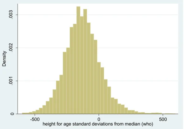
Of the 38,193 observations for HAZ score in the dataset, 11,191 values indicate malnutrition (HAZ score below -200 i.e. -2×100) representing 29.32% of the total observations. 70.68% of these observations in the dataset are not considered stunted (a histogram showing the distribution of numerical data of the dependent variable -HAZ is presented in Appendix as figure A1). The average age of children in the dataset used is 1.99 years.

Child mortality rate is another variable of interest considered in this analysis. Here, I analyse child deaths per 1000 births within Kenya between 1998 to 2014 using 2003, 2008 and 2014 survey years. The main measure of mortality is an indicator for whether a child died at the age of 5 or younger, referred to as under-five mortality rate (U5MR). U5MR is constructed from a set of questions posed by KDHS survey personnel to women aged 15-49 about children born in the 5 years before the survey (i.e., the number of children who live with the respondent, those who live elsewhere, and the number who have died). Responses to these questions are used to construct retrospective birth and death histories for all children in the dataset. The complete fertility histories are then used to directly estimate U5MRs. With this, we can examine how U5MRs have evolved overtime in Kenya. In the dataset, U5MRs are given as 115, 74 and 52 deaths per 1000 live births for 2003, 2008 and 2014 survey years respectively

13_{In their analysis, Ferreira & Schady (2009) review literature on Aggregate Economic Shocks, Child}

Schooling and Child Health. Reviewed literature shows that height-for-age is widely used as a measure of the nutritional status of children.

(25)

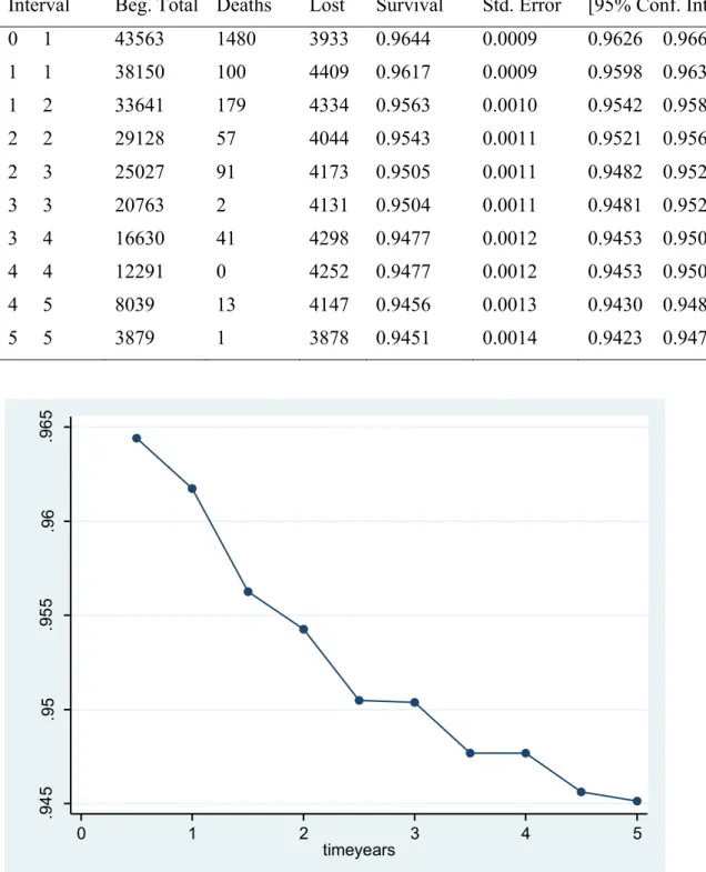
(see table A1 in Appendix). During the survey, antenatal record book is used to confirm the events of child birth for women who attended clinics. Information on children born or died more than 5 years prior to the survey years is discarded. This helps to minimize recall bias. Based on the guidelines set out by O’Donnell et al., (2007)14_{, I compute mortality and a} cumulative survival function using the pooled KDHS dataset. From the data set, I use Century Month Code (CMC) for the date variables. These variables (date of interview (CMC); child’s date of birth (CMC); child's age at death in month (including imputed); and whether child is alive) are needed for direct mortality estimation when using DHS datasets. I use Stata to generate actual surviving time (in years) for each child in the pooled dataset. I compute the status variable mortality based on the variable of whether child is alive or not. Using surviving time and mortality variables in Stata, I construct a life table which is then used to compute the U5MR for the pooled dataset (details in Appendix- Table A2). Out of the 43,753 observations, deaths recorded are 2,154. From the population sample for children under the age five used in this study, average mortality (deaths) is 4.9% (Table 1: summary statistics).

I include control variables for child, parental and household characteristics in the model. These will enable control for confounders in the model and are based on previous research findings Previous studies show that child characteristics such as birth order number, multiple births and sex of child have a significant effect on child health outcomes (Horton, 1988; Kabubo-Mariara et al., 2009) and thus these variables are included in the model. Parental characteristics (i.e. mother’s age, maternal education and parental occupations) are included and controlled for due to their impact on child health outcomes (c.f. Paxson & Schady, 2005; Baird et al., 2011; Finlay et al., 2011; Benshaul‐Tolonen, 2018). Dummy variables on whether the father or mother are employed in the agricultural sector are also included because vulnerability to commodity fluctuations should be more pronounced among children born to agricultural parents. Household characteristics such as rural/urban status, household head and wealth are also included. A wealth index is used to describe the relative wealth of the household where mother and child reside based on quintiles. Quintiles are divided into poorest, poorer, middle, richer and richest. Without data on household incomes and consumption per capita, tea revenue and household wealth index are instead used as proxies. The regression equations above, clarify on the exact variables used in each specification.

(26)

6.3. Tea Growing Zones

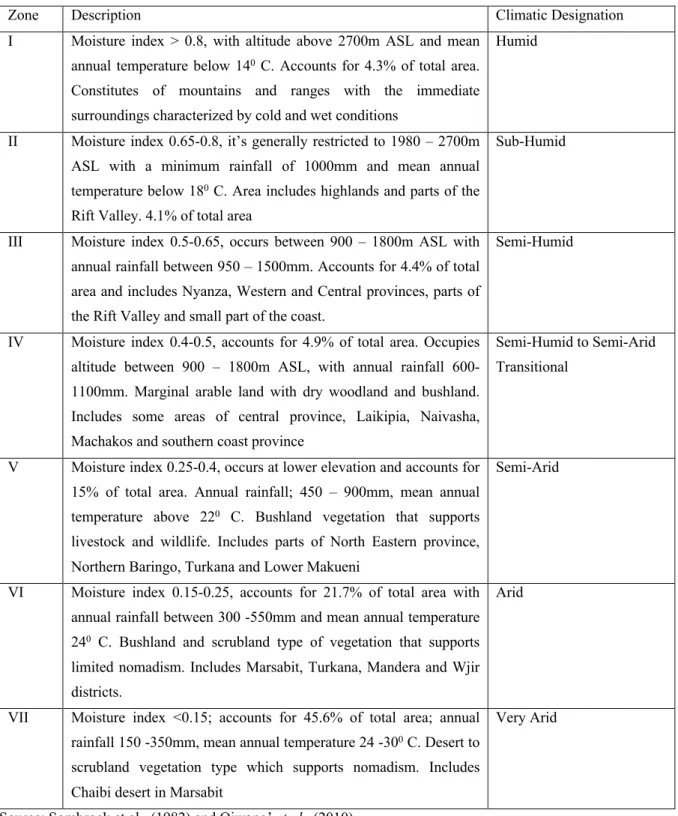
To classify tea growing zones of Kenya, I use a moisture index developed by Sombroek et al., (1982). The moisture index is based on annual rainfall expressed as a percentage of annual transpiration, and he used it to divide Kenya into seven agro-climatic zones (refer to Appendix- table A3). Different land uses are assessed based on climate, vegetation, and soil conditions. Variations, intensity, and duration of rainfall as well as evapotranspiration affect soil moisture which influences plant growth and vegetation at any site. Based on the exploratory soil map, agro-climatic zones and AEZ maps of Kenya, I identify areas suitable for tea cultivation and these are used as a baseline indicator for presence of tea in a zone.

Using QGIS15_{, I merge DHS geographic datasets with the AEZ geographic dataset thus} matching AEZs with the location of survey clusters. I use an AEZ shapefile based on temperature and crop suitability of Kenya (ILRI - GIS Services) combined with information on altitude and moisture index to identify areas suitable for tea growing. This information is then merged with the DHS geographic dataset using the GPS coordinates to match surveyed households to tea growing zones. The merged dataset is then converted into a shapefile and transformed into a STATA file16_{which is then merged with the DHS dataset using the DHSID}17 variable. With this, households or clusters surveyed are ultimately classified as being situated in tea growing zone or not.

DHS data used is pooled cross-sectional data, i.e. it deals with observation of different subjects in different time periods (2003, 2008 and 2014). The pooled cross-sectional DHS data set merged with AEZs and the tea price datasets has 43,753 number of observations. The total number of observations in the pooled cross-sectional dataset is different for all variables due to missing or inconsistent data in the surveys. A summary of variables contained in constructed data set is presented in table 1 below.

15_{https://www.qgis.org/en/site/ (}_{QGIS is a geographic information system (GIS) application software)} 16_{shp2dta reads a shape (.shp) and dBase (.dbf) file from disk and converts}

them into Stata datasets. Refer to https://www.stata.com/support/faqs/graphics/spmap-and-maps/

17_{A 14 character DHS identification code, refer to}_{https://dhsprogram.com/What-We-Do/upload/MEASURE-}

(27)

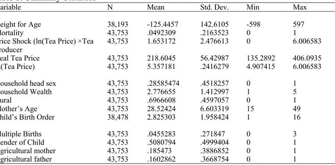
Table 1: Summary Statistics

Variable N Mean Std. Dev. Min Max

Height for Age 38,193 -125.4457 142.6105 -598 597 Mortality 43,753 .0492309 .2163523 0 1 Price Shock (ln(Tea Price) ×Tea

Producer 43,753 1.653172 2.476613 0 6.006583 Real Tea Price 43,753 218.6045 56.42987 135.2892 406.0935 ln(Tea Price) 43,753 5.357181 .2416279 4.907415 6.006583 Household head sex 43,753 .28585474 .4518257 0 1 Household Wealth 43,753 2.776655 1.412997 1 5 Rural 43,753 .6966608 .4597057 0 1 Mother’s Age 43,753 28.52424 6.603319 15 49 Child’s Birth Order 38,478 2.825303 1.958424 1 16 Multiple Births 43,753 .0455283 .271847 0 3 Gender of Child 43,753 .5080794 .4999404 0 1 Agricultural mother 43,753 .185473 .3886852 0 1 Agricultural father 43,753 .1602862 .3668754 0 1

Note: Individual level data from KDHS 2003, 2008 & 2014 for children under 5 years of age born to mothers between ages of 15-49 between 1998-2014.

(28)

7. Results and Discussion

In this section, I report the main estimates of equations (1) and (2) from chapter 4 in Table 2 and 3. In column (1) of table 2 and 3, are results from the baseline specifications for both height for age and mortality under five respectively. Results in column (2) are of the new specifications that allow for zone specific time trends. Expanded results with the interaction term between Tea Price Shock and parental occupation (father and mother) dummy variables are presented in columns (3). Standard errors clustered at DHS cluster level are indicated in parentheses.

(29)

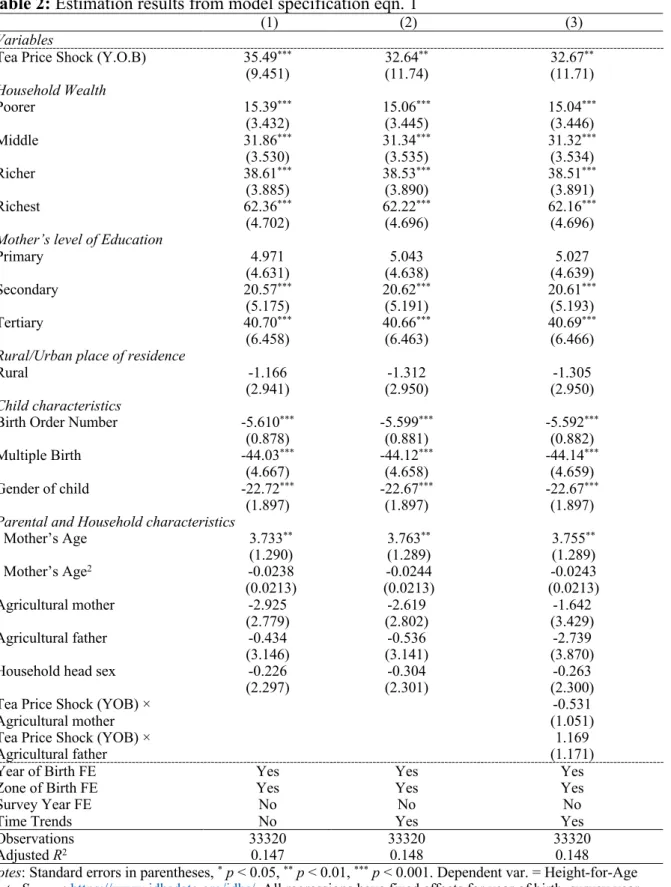
Table 2: Estimation results from model specification eqn. 1

(1) (2) (3)

Variables

Tea Price Shock (Y.O.B) 35.49***

(9.451) 32.64 ** (11.74) 32.67 ** (11.71) Household Wealth Poorer 15.39*** (3.432) 15.06 *** (3.445) 15.04 *** (3.446) Middle 31.86*** (3.530) 31.34 *** (3.535) 31.32 *** (3.534) Richer 38.61*** (3.885) 38.53 *** (3.890) 38.51 *** (3.891) Richest 62.36*** (4.702) 62.22 *** (4.696) 62.16 *** (4.696)

Mother’s level of Education

Primary 4.971 (4.631) (4.638) 5.043 (4.639) 5.027 Secondary 20.57*** (5.175) 20.62 *** (5.191) 20.61 *** (5.193) Tertiary 40.70*** (6.458) 40.66 *** (6.463) 40.69 *** (6.466)

Rural/Urban place of residence

Rural -1.166

(2.941) (2.950)-1.312 (2.950)-1.305

Child characteristics

Birth Order Number -5.610***

(0.878) -5.599 *** (0.881) -5.592 *** (0.882) Multiple Birth -44.03*** (4.667) -44.12 *** (4.658) -44.14 *** (4.659) Gender of child -22.72*** (1.897) -22.67 *** (1.897) -22.67 *** (1.897)

Parental and Household characteristics

Mother’s Age 3.733** (1.290) 3.763 ** (1.289) 3.755 ** (1.289) Mother’s Age2 _-0.0238 (0.0213) (0.0213)-0.0244 (0.0213)-0.0243 Agricultural mother -2.925 (2.779) (2.802)-2.619 (3.429)-1.642 Agricultural father -0.434 (3.146) (3.141)-0.536 (3.870)-2.739 Household head sex -0.226

(2.297) (2.301)-0.304 (2.300)-0.263 Tea Price Shock (YOB) ×

Agricultural mother (1.051)-0.531

Tea Price Shock (YOB) ×

Agricultural father (1.171)1.169

Year of Birth FE

Zone of Birth FE Yes Yes Yes Yes Yes Yes

Survey Year FE No No No

Time Trends No Yes Yes

Observations 33320 33320 33320

Adjusted R2 _0.147 _0.148 _0.148

Notes: Standard errors in parentheses, *_{p < 0.05,}**_{p < 0.01,}***_{p < 0.001. Dependent var. = Height-for-Age}

Data Source: https://www.idhsdata.org/idhs/ All regressions have fixed effects for year of birth, survey year and zone of birth unless otherwise indicated. To the basic specification of eqn. 1, the variable Time trends (expressed in zone-specific time trends) is added and results are presented in column (2). In column (3), results shown include an addition of interaction variables to the new model specification with time-trends

(30)

7.1. Child Nutritional Status

To begin with, I evaluate the effect of tea price shock on child nutritional status using height-for-age Z (HAZ) score as a proxy following standard literature (Hoddinott & Kinsey, 2001; Maluccio, 2005; Yamano et al., 2005; Alderman et al., 2009; Cogneau & Jedwab, 2012). Under the main specification in equation (1), results indicate that a 1% change in the real producer price of tea generates an increase in the HAZ score by 35.49 standard deviations above the median height (column 1) among children born in tea growing zones. The effect is statistically significant at 1% error level. However, once the model specification accounts for time trends (column 2) and the interaction between tea price shock and dummy variables on whether the father or mother are employed in the agricultural sector (column 3), the impact reduces. A one percent increase in price is associated with 32.64 and 32.67 standard deviation improvements in child nutritional status relative to the reference median respectively. The estimated coefficients are still statistically significant across all specifications (columns 2 and 3).

Household income is a vital determinant of child health status. A positive change in real producer price of tea boosts a household’s income earning potential and overall wealth which leads to more resources being available at time of birth to children born in tea growing zones. Households in tea growing zones can make child health investments through the consumption of health promoting goods. The results attained here on height-for-age score are analogous to findings in Ivory Coast by Jensen (2000) and Cogneau & Jedwab (2012). Jensen (2000) observes that negative weather shocks such as drought negatively affect household income, causing a reduction in child health investments which in turn increases the risk of malnutrition. Also, by exploiting a negative income shock in-form of a reduction in cocoa prices, Cogneau & Jedwab (2012) discover a decline in HAZ for children between 2-4 years of age in cocoa growing areas. This is consistent with my results above, where I use pooled OLS estimate with fixed effects to analyse the impact of tea price shock at time of birth on child nutritional status and find that an increase in tea price is associated with HAZ score improvement for children born in tea growing zones.

The variable household wealth is a composite measure of a household's cumulative living standard or wealth and it is divided into quintiles (see subsection 6.2 above). Household wealth is statistically significant at 1% error level across all results- column (1), (2) and (3). Children

(31)

from households in poorer, middle, richer and richest quintiles have HAZ scores of 15.39, 31.86, 38.61 and 62.36 standard deviations higher than children from households in the poorest quintile (i.e. the reference category) respectively. Therefore, children born into wealthiest households in tea growing zones are the least likely to be stunted and have better nutritional status. This is contrasts the findings of Yamano et al., (2005) who uses a variety of assets to represent household wealth and finds the variable to be insignificant. This is not the case here, as I use a wealth index computed from survey data and is a representative measure of a household’s total assets.

Mother’s level of education is significant at both secondary and tertiary education level in comparison to no education. Education is insignificant at primary education level with an estimated coefficient of 4.97. Primary education level being a prerequisite for secondary education, low quality of education services and poor primary school attendance levels are some of the factors that can be used to explain the small coefficient estimated for primary education. On the other hand, higher and secondary education levels have 40.7 and 20.57 estimated coefficients respectively for the baseline specification column (1). These results suggest that maternal education has a statistically significant impact on child nutrition. Considering time-trends and the interaction between tea price shock and dummy variables on whether the father or mother are employed in the agricultural sector, estimated coefficients are significant for secondary and tertiary education column (2) and (3) and there is little change with results from the baseline specification. The results at primary level are still insignificant. Educated mothers are more likely to use modern health care, have good health care knowledge and reproductive behaviours. Yamano et al., (2005) finds that limited maternal education exacerbates the prevalence of stunting among Ethiopian children. Although they use a household education status proxy by using the highest grade attained by the most educated male and female in the household as opposed to maternal education level as used here. Their conclusion is identical to the interpretation of estimated results in Table 2, that women empowerment (education) has a positive impact on child health and welfare.

Mother’s age estimates show that it is positively associated with child’s nutritional status, the estimated coefficient is 3.733 under the basic regression column (1). Mother’s age is associated with a 3.73 standard deviations improvement in the HAZ score for a child born in the tea growing zones. The estimated coefficients for mother’s age are significant across all samples. Under the more rigorous regressions, estimated coefficients are both 3.76 (columns 2 and 3) and are still statistically significant. Given that the mean age of mothers in the pooled data set

(32)

used is 28.52, the findings are similar to Finlay et al., (2011) who concludes that the risk of poor child health outcome is lowest among women who have their first birth between the ages of 27-29 and observed that children of adolescent mothers are the most vulnerable to poor health outcomes due to biological and social factors at play.

Child birth order has negative effects on nutritional status, with HAZ score declining with the increase in birth order number of children. Birth order is associated with a 5.61 decline in nutritional status of child born in the tea growing zones. The results show a slight change in the estimated coefficients once time-trends and the interaction between tea price shock and dummy variables on whether the father or mother are employed in the agricultural sector have been accounted for (columns 2 and 3 respectively). The estimated coefficients are statistically significant for all specifications. These results supports the conclusion of a previous study by Horton, (1988), who finds that child birth order has a significant impact on child nutritional status. This impact is found to be negative.

In the tea growing zones, children of multiple births are associated with a decline in HAZ score of 44.03 standard deviations in comparison to singletons under the baseline specification (column 1). With time-trend and interaction between tea price shock and dummy variables on whether the father or mother are employed in the agricultural sector accounted for in the rigorous model specifications, there is a decline in HAZ score for children of multiple births by 44.12 and 44.14 standard deviations respectively (columns 2 and 3). All results are statistically significant. These results could be explained by low birth weight, inadequate breast feeding and competition for nutritional food, factors which are common among most children of multiple births. The results confirm the findings of Kabubo-Mariara et al., (2009), with children of multiple births found to be more likely malnourished in comparison singletons. The variable gender indicates that the male child is associated with a decline in HAZ score of 22.72 standard deviations under the baseline specification column (1) in comparison to the female child. Taking time-trends and the interaction between tea price shock and dummy variables on whether the father or mother are employed in the agricultural sector into account, the coefficient is estimated at 22.67 respectively (columns 2 and 3). The impact is significant at 5% level across the surveyed population. This result is identical to Kabubo-Mariara et al., (2009)’s study that shows that in Kenya male children are more likely to be stunted compared to their female counterparts.

(33)

Father and mother’s employment maybe an important determinant of child health status. The results in table 2 show that children whose parents are agricultural workers are associated with a negative change in standard deviations for height-for-age scores. However, both estimated coefficients for agricultural mother and father are not significant. This may be explained by other factors at play such as the presence of respondents who answered “currently not working” in the survey dataset. These constituted between 20 – 45.07% of the total respondents across survey years examined. Employment figures18_{show that over 70% of Kenya’s rural population} is actively engaged in agriculture and over 80% rely on it as a source of livelihood in form of subsistence and commercial farming. Ordinarily, subsistence/smallholder farmers are more likely not to consider farming as source of employment and respond negatively to the survey question. Seasonal farm labour would probably have responded negatively to the survey question depending on when the survey was carried out.

Furthermore, the coefficients of the interaction between agricultural mother, and father and the price shock variable are small and non-significant. The variables; gender of household head and rural are insignificant across all estimates irrespective of the model specification used.

(34)

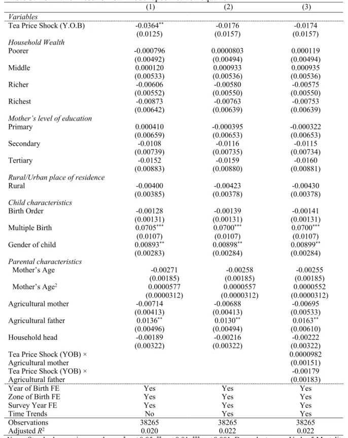
Table 3: Estimation results from model specification equation 2

(1) (2) (3)

Variables

Tea Price Shock (Y.O.B) -0.0364**

(0.0125) (0.0157)-0.0176 (0.0157)-0.0174 Household Wealth Poorer -0.000796 (0.00492) 0.0000803 (0.00494) (0.00494) 0.000119 Middle 0.000120 (0.00533) (0.00536) 0.000933 (0.00536) 0.000935 Richer -0.00606 (0.00552) (0.00550)-0.00580 (0.00550)-0.00575 Richest -0.00873 (0.00642) (0.00639)-0.00763 (0.00639)-0.00753

Mother’s level of education

Primary 0.000410 (0.00659) -0.000395(0.00653) -0.000322(0.00653) Secondary -0.0108 (0.00739) (0.00735)-0.0116 (0.00734)-0.0115 Tertiary -0.0152 (0.00883) (0.00880)-0.0159 (0.00881)-0.0160

Rural/Urban place of residence

Rural -0.00400 (0.00385) (0.00378)-0.00423 (0.00378)-0.00430 Child characteristics Birth Order -0.00128 (0.00131) (0.00131)-0.00139 (0.00131)-0.00141 Multiple Birth 0.0705*** (0.0107) 0.0700 *** (0.0107) 0.0700 *** (0.0107) Gender of child 0.00893** (0.00283) 0.00898 ** (0.00284) 0.00899 ** (0.00284) Parental characteristics Mother’s Age -0.00271 (0.00185) (0.00185)-0.00258 (0.00185)-0.00255 Mother’s Age2 _0.0000577 (0.0000312) (0.0000312)0.0000557 (0.0000312)0.0000552 Agricultural mother -0.00714 (0.00413) (0.00413)-0.00688 (0.00533)-0.00695 Agricultural father 0.0136** (0.00496) 0.0130 ** (0.00494) 0.0163 ** (0.00610) Household head -0.00189 (0.00322) (0.00322)-0.00216 (0.00322)-0.00222 Tea Price Shock (YOB) ×

Agricultural mother 0.0000982(0.00151) Tea Price Shock (YOB) ×

Agricultural father (0.00183)-0.00179

Year of Birth FE

Zone of Birth FE Yes Yes Yes Yes Yes Yes

Survey Year FE Yes Yes Yes

Time Trends No Yes Yes

Observations 38265 38265 38265

Adjusted R2 _0.020 _0.022 _0.022

Notes: Standard errors in parentheses, *_{p < 0.05,}**_{p < 0.01,}***_{p < 0.001. Dependent var. = Under-5 Mortality}

Data Source: https://www.idhsdata.org/idhs/ All regressions have fixed effects for year of birth, survey year and zone of birth unless otherwise indicated. To the basic specification of equation 2, the variable Time trends (expressed in zone-specific time trends) is added and results are presented in column (2). Column (3) shows results after the addition of interaction variables to the new model specification with time-trends.