NORTRIP
NOn-exhaust Road TRaffic Induced
Particle emissions
Development of a model for assessing the effect on air
quality and exposure
Christer Johansson, (project coordinator),
Department of Applied Environmental Science (ITM), Stockholm University Bruce Rolstad Denby1, Ingrid Sundvor1, Mari Kauhaniemi2, Jari
Härkönen2, Jaako Kukkonen2, Ari Karppinen2, Leena Kangas2,
Gunnar Omstedt3, Matthias Ketzel4, Andreas Massling4,Liisa
Pirjola5, Michael Norman6, Mats Gustafsson7, Göran Blomqvist7,
Cecilia Bennet7, Kaarle Kupiainen8,9 , Niko Karvosenoja9
1The Norwegian Institute for Air Research (NILU). Kjeller, Norway. 2Finish Meteorological Institute (FMI), Helsinki, Finland.
3Swedish Meteorological and Hydrological Institute (SMHI), Norrköping, Sweden. 4Department of Environmental Science (ENVS/AU), Aarhus University, Denmark. 5Helsinki Metropolia University of Applied Sciences, Finland.
6Environment and Health Administration, Stockholm, Sweden.
7Swedish National Road and Transport Research Institute (VTI), Linköping, Sweden. 8Nordic Envicon Oy, Helsinki, Finland.
9Finnish Environment Institute (SYKE), Helsinki, Finland.
Partly financed by Nordic Council of Ministers
June 2012
ITM-report 212
Department of Applied Environmental Science
Institutionen för tillämpad miljövetenskap
Content
1. Preface ... 1
2. Summary ... 2
2.1 Background and aim ... 2
2.2 Features of the model ... 2
2.3 Model parameters and evaluation ... 3
2.4 Main conclusions ... 3
2.5 Remaining issues and recommendations of further studies ... 4
3. Introduction ... 6
4. Aims ... 6
5. Model description ... 6
6. Datasets and supporting information for process modeling ... 9
6.1 Emission factors for road wear... 13
6.2 Emission factors based on mobile laboratory measurements ... 13
6.3 Wind induced suspension ... 17
6.4 Sandpaper effect... 17
6.5 Importance of accurate surface moisture modeling ... 18
6.5.1 Road surface wetness measurements ... 18
6.5.2 Modeling of surface wetness ... 20
6.6 Importance of road salt ... 24
6.6.1 Application of the NORTRIP model to RV4, Oslo ... 24
6.6.2 Application to Hornsgatan, Stockholm ... 25
6.7 Spray and splash ... 27
6.8 Model sensitivity to sanding ... 28
6.9 An evaluation of predicting sanding and salting ... 28
7. Results from applications of the model ... 30
7.1 Effect of reduced studded tyre use on Hornsgatan on concentrations of PM10 ... 30
7.2 Evaluation of reduced vehicle speed in Oslo ... 32
7.3 Comparison of NORTRIP and SMHI models ... 34
8. Remaining research questions and recommendations ... 34
9. References ... 36
10. Appendix 1. Reports with contributions from the NORTRIP project ... 39
11. Appendix 2. Conference abstracts ... 41
12. Appendix 3. Comparison between two models ... 59
1. Preface
This is a summary report of a research project that has been partially financed by the Nordic Council of Ministers (NMR). The contact at Nordic Council of Ministers has been Hans Skotte Møller, working group on Climate and Air Quality. Other support for the work has been through an EU project, TRANSPHORM "Transport related Air Pollution and Health impacts – Integrated Methodologies for Assessing Particulate Matter", with FMI and NILU as partners, and through several national agencies in the Nordic countries.
The project is called NORTRIP, which is also the name of the non-exhaust emission model that has been developed within this two year project (2010-2012). The project has involved 18 researchers from Sweden, Norway, Finland and Denmark (see list of co-authors of this report).
Stockholm, June 2012
Christer Johansson, project coordinator Professor
Atmospheric Science unit
Department of Applied Environmental Science Stockholm university
2. Summary
2.1 Background and aim
The PM10 concentrations exceed the EU limit values in almost all countries in Europe. Up to 49 percent of the European urban population is exposed to PM10 concentrations in excess of the EU daily air quality limit value, and there is no downward trend in most cities. Non-exhaust particle emissions make an important and increasing contribution to PM10 concentrations in cities. Especially, in many Nordic cities, non-exhaust particle emissions are the main reason for high PM10 levels along densely trafficked roads. This is connected to the use of studded tyres and winter time road traction maintenance, e.g. salting and sanding.
The ultimate aim of the project has been to develop a process based emission model, that can be applied in any city without site specific empirical factors, for management and evaluation of abatement strategies and that is able to describe the (non-exhaust) emissions on an hourly or at least daily basis with satisfactory accuracy.
2.2 Features of the model
The model developed within the NORTRIP project is built upon existing road dust emission models, combined with field and laboratory measurements. It is a comprehensive model based on generalised processes describing the non-exhaust emissions. The major features of the model are:
Road dust and salt loading is calculated based on a mass balance equation.
Production of road dust, and subsequent emissions, are based on the total wear of road, brakes and tyres.
Maintenance activities (e.g. salting, sanding, cleaning, ploughing) contribute to the mass balance as well as processes such as drainage and splash/spray.
Retention of road surface dust is dependent on the surface moisture content.
The road surface moisture is calculated based on a mass balance equation for surface water and ice.
Evaporation is based on energy balance modelling of the road surface.
Maintenance activities (e.g. cleaning, ploughing, salt solutions) and processes (e.g. drainage, splash/ spray) are included in the moisture mass balance
The impact of salting on both dust retention and melt temperature is considered
Compared to earlier non-exhaust models, a number of important improvements have been made. For example, in the surface road moisture calculation, the effects of salt on evaporation and condensation, and the effect of buildings and vehicles on the energy balance. The NORTRIP model may also be run using relative measurements of road surface moisture in order to facilitate evaluation of abatement strategies, such as a studded tyre ban or speed reduction. Another important improvement is the identification and separation of the controlling processes so that abatement strategies and influencing factors can be easily evaluated. The separation of direct wear emission processes and indirect emissions due to suspension is particularly important as they are controlled by different processes. The NORTRIP model is programmed in MATLAB, but easily run and controlled via excel and all output and input values are stored in a common excel sheet for further analyses.
2.3 Model parameters and evaluation
Most probable values for the model parameters have been obtained from results of several laboratory and field studies as well as from literature reviews. PM10 and PM2.5 measurements in a road simulator (at VTI, Linköping) have provided direct road wear emission factors
depending on tyre and pavement type and vehicle speed. Suspension rates and its dependence on vehicle type and speed has been obtained from on-road measurements using mobile laboratories and tuning of model parameters based on comparison with measurements at kerbside sites. Literature data has been used to estimate key parameters for describing tyre and brake wear. Various parts of the model have been tested and applied to datasets from Stockholm, Oslo, Helsinki and Copenhagen. A complete description of the model and its parameter determination is contained in a parallel NILU report by Denby and Sundvor (2012).
The performance of the model has been assessed by comparison between modelled and measured dust load, salt load, surface temperature, surface moisture and PM10 concentrations. The model has been applied to evaluate two specific abatement measures to reduce PM10 emissions; the ban on studded tyres in Stockholm and the reduced speed on an arterial road in Oslo. Additional applications of the model are ongoing and planned. The NORTRIP model reproduces measured concentrations, with satisfactory accuracy, for most of the datasets assessed.
2.4 Main conclusions
The project has involved close co-operation between researchers in the Nordic countries and resulted in several publications and conference presentations. The main conclusions are:
- A new improved non-exhaust emission model, called NORTRIP, has been developed, tested and applied on data from road simulator studies, on-road emission measurements and ambient, kerbside datasets from Stockholm, Oslo, Helsinki and Copenhagen. - The NORTRIP model is currently the most comprehensive process based non-exhaust
emission model available. It provides not just a means for predicting non-exhaust
contributions to PM concentrations but also a platform for understanding and controlling these emissions.
- The model successfully reproduces measured concentrations, with satisfactory accuracy, for most of the datasets assessed and, in some cases, the model exceeds expectations. This is particularly true for simulations of Hornsgatan in Stockholm which provides the best set of data for model development and assessment.
- Modelling both dust loading and road moisture is essential for accurately simulating hourly mean PM10 emissions.
- Measurements on Hornsgatan (Stockholm) have shown that road moisture is the most important factor that controls the temporal variability of the PM10 emissions; wet periods lead to low emissions and accumulation of dust that is suspended as roads dry out.
Accurate modelling of road moisture is therefore one of the most crucial model parameters for predicting PM10 concentrations.
- The accuracy of the road moisture modelling was assessed by comparison with measured road moisture in Stockholm (relative variation) and Copenhagen (absolute moisture). Typically (for Hornsgatan, Stockholm) the correlation between measured and modelled daily mean PM10 values was between 0.4 and 0.6 when road moisture was calculated, and it increased to between 0.8 and 0.9 when measured road moisture was used. - Including road salt has been shown to improve modelling of road wetness as salt lowers
the vapour pressure, which keeps the road surface wet for a longer time. The agreement between measured and modelled PM10 increased significantly when salt was added
(shown for Copenhagen, Oslo and Stockholm). Road salt may also contribute to PM10 mass concentration as seen in data from Oslo. The impact of road salt on PM10
concentrations has been assessed by comparison of modelled road salt contribution and measured concentration in PM10. In Oslo road salt could contribute with up to 16%of the total concentrations in the winter period.
- Prediction of sanding events based on meteorological criteria was in very poor agreement with real sanding events as shown by comparisons between predicted and actual events in Helsinki. Other factors, such as decisions on the need for sanding by local road
maintenance officers base on other factors than meteorological forecasts, is difficult to consider in a model.
- The impact of road sanding on PM10 was assessed using the model for the one winter period when sanding data was available. It was found that most of the variability and the mean concentrations could be explained without sand as a contributing factor. For
Hornsgatan where some sanding data is available, the model indicates that sanding does not contribute more than around 10% of the annual mean concentrations but may contribute to the number of exceedance days.
- The importance of a ban on studded tyres for the PM10 emissions and concentrations could be separated from other influencing factors such as road wetness, reduced traffic and shorter period when studded tyres is allowed. The reduced use of studded tyres and a shorter period in which the use of studded tyres is allowed, was estimated to have reduced PM10 concentrations by 6.7 and 13.7 μg m-3, for the period 1 Jan to 31 May 2010 and
2011, respectively. This corresponds to a reduction of 14% (2010) and 25% (2011) of the total PM10 concentrations for a reduction in studded tyres use from 65% to 40% and from 65% to 35% in 2010 and 2011, respectively.
- The impact of a reduction in speed limit on PM10 emissions and concentrations along an arterial road in Oslo was evaluated using the model. Model results showed that there were a number of contributing factors, not just speed, to the apparent reduction in concentrations between the two years. Speed reduction contributed around 10% of a total 25% reduction.
- A comparison using one year of data from Hornsgatan shows that the NORTRIP model gives a higher correlation coefficient than the SMHI model (i.e. reproduces the phase better), while the SMHI model reproduces the standard deviation better (i.e. the amplitude). There are a number of differences between the models, but the main difference is that the NORTRIP model has more detailed parameterization of processes and is developed to understand the underlying controlling processes, not just calculate PM10 concentrations.
2.5 Remaining issues and recommendations of further studies
The NORTRIP model has been developed with the main aim of improving our understanding of non-exhaust emissions for air quality management applications. The procedure was to identify a number of important processes, even if these cannot be well defined with current knowledge, and implement these in a conceptual and mathematical modelling tool. As such there are some poorly defined processes, e.g. crushing and abrasion, which are not currently included in the model applications but are described within the model structure. Other processes such as suspension rates did not show the expected dependence on vehicle speed. If these are to be improved upon then additional existing databases, particularly outside of Nordic countries, need to be acquired and the model applied and tested on these to assess the robustness of the model concept and its implementation.
A number of the parameters used in the model are still poorly defined. Recent studies indicate that pavement texture is an important parameter for both dust loading and suspension, but more
experimental data is needed to clarify this. Further measurements of processes, such as road dust/salt loading and suspension rates, are required for improving these. Activity data (on sanding, salting, dust-binding etc.) is required but is seldom easily available. Better prognoses or other means for modeling sanding activities is needed. Street cleaning using current sweeping, vacuuming and water flushing techniques is inefficient for reducing PM10, but simple model tests indicates that there are potential benefits if the dust depot could be reduced efficiently. But this requires further experimental verification.
A number of measurements, both laboratory and field measurements, are identified that would greatly help improve the model and its process descriptions.
3. Introduction
Up to 49 percent of the European urban population is exposed to PM10 concentrations in excess of the EU daily air quality limit value, and in general there is no downward trend (EEA, 2011). In many European cities non-exhaust particles contribute equally or more to total traffic-related emissions than exhaust particles and they are of increasing importance for the exposure (e g Thorpe and Harrison, 2008). Technological improvements and stricter regulations will continue to decrease exhaust emissions, while non-exhaust emissions are essentially unregulated so far. There is an acute need for improved information on these sources for policy to advance.
Non-exhaust emissions are mainly due to abrasion processes and suspension of particles from dry road surfaces in the wake of passing vehicles. The most important abrasion processes that lead to direct emissions of particles are wear of brakes, tyres and road surfaces (Thorpe & Harrison, 2008; Boulter, 2005). Different non-exhaust particle sources contribute to both fine and coarse particles (e g Boulter, 2005; Wahlström et al., 2010), as well as ultrafine particles (Dahl et al., 2006; Kumar, et al., 2012).
An increasing number of studies show their potential negative health impacts. Coarse particle exposure in Stockholm, mainly caused by road abrasion, is significantly associated with
premature mortality and affects respiratory and cardiovascular morbidity (Meister et al., 2012). Toxicological effects of road pavement wear has been documented (e g Gustafsson et al., 2008), brake wear (Gasser et al., 2009) and tyre wear particles containing high aromatic oils may potentially contribute to the carcinogenicity of particulate matter (Sadiktsis et al., 2012). The ability to model these emissions is highly desirable as this provides the potential for more effective air quality management, quantification of the impact of mitigation activities and
estimation of population exposure for assessment of health impacts. But this is a challenging task as the emissions depend on a number of environmental and technological factors. Models used to predict traffic induced suspension emissions are based on relatively little data. For any
improvement in these models (which in principle can describe the effect of abatement measures) more extensive high-quality data from both field and laboratory studies is required.
4. Aims
The ultimate aim of the project has been to develop a process based emission model, that can be applied in any city without site specific empirical factors, for management and evaluation of abatement strategies and that is able to describe the (non-exhaust) emissions on an hourly or at least daily basis with satisfactory accuracy. Specifically, the new model should fulfill the needs of an accurate modeling tool for quantification of non-exhaust emissions for Nordic road traffic conditions.
5. Model description
The NORTRIP model is based on the work previously carried out by Berger and Denby (2011) but has undergone a large number of changes as a result of activities in NORTRIP, both in terms of model development and improvements in the definition of model parameters. The model concept also has a strong basis in the model from Omstedt et al. (2005), where the concept of surface mass balance for dust and moisture was first developed. Using a combination of field and laboratory measurements, a more comprehensive and generalized process based model has been developed. Key features:
The model can predict as well as possible the vehicle induced road dust, and other
non-exhaust, emissions for a range of road types in the urban environment (not just a
single road)
The model can be used for air quality management purposes (to assess measures)
It is modelling tool that is portable (is sufficiently universal for it to be applied in a
variety of environments)
It is a conceptual tool, which describes the range of processes involved in road dust
emissions, providing an overview of these processes and their likely dependencies.
This means that the model should function as well as possible for a variety of roads, even where there is no data available for empirical correction. It describes processes that are relevant for any mitigation strategy and that may influence the emissions. The model may be used to assess impact on PM10 of vehicle speed, road salting, vehicle type, tyre type, road surface types and various activities such as street cleaning, salting and dust binding.
The basic emission processes determined by the model are direct emissions due to road wear, direct emissions due to other wear sources and indirect emissions (suspension) of road dust either mechanically by vehicle wheels or by vehicle or wind induced turbulence. The complexity and variety of processes that may be very different in different environments is illustrated by the key processes involved in Figure 1. The sinks and sources of road surface material (including salt) and moisture is calculated at every time step to keep track of the total dust and moisture load on the road.
The performance of the model has been assessed by comparison between modelled and measured dust load, salt load, surface temperature, surface moisture and PM10 concentrations.
Figure 1. Schematic outline of the NORTRIP emission model.
The model is programmed in MATLAB1 but can be run from Excel. Input and ouput data is stored
in Excel. Since this is an emission model without any atmospheric dispersion calculation, it requires NOx or some other tracer to convert emissions into concentrations. This can also be done if the dispersion is estimated by other methods, e g using a dispersion model. The data required and/or desired to run the model is listed in Table 1.
Table 1. Data required and/or desired to run the model.
Degree of data requirement
Meta data Meteorological
data Road wear and suspension
parameters
Road moisture Concentration data
Activity data
Mass balance
data Other data
Required data Road and building configuration, street direction, surface albedo
Wind speed and direction, relative humidity, global radiation (or cloud cover)
Traffic flow, HDV share, studded tyre share, sign posted speed
Meteorological data from urban background station
Street level and background concentrations of NOx for converting the PM emissions to PM concentrations (alternatively other estimates of atmospheric dispersion may be used) Exhaust emission factor in order to get total PM10 emissions (and concentrations)
Not required, but improves model results significantly Pavement properties (especially if studded tyres are used). Measured vehicle speed.
Surface moisture measurements
PM10 and PM2.5 data for validation.
Dust binding, road salting and sanding activities
Road dust layer and salt loading Concentrations in surface water and drainage water
Not required but might improve model results if data quality is good Road surface temperature, wind speed at street level, salt content of road dust layer, cleaning and salting activities, splash and spray data
Cleaning activities, ploughing activities
6. Datasets and supporting information for
process modeling
A number of datasets have been used to quantify the various parameters involved in describing the basic processes as well as for model validation. Sources of data for model parameters are summarized in Table 2 and an overview of the datasets is given in Table 3. References and details on how this information was used to obtain parameterizations are described in the NORTRIP model documentation (Denby and Sundvor, 2012).
Data from laboratory studies using road simulators and experiments using mobile laboratories in Sweden and Finland have provided basic information on the road wear, suspension and
importance of sanding and dust load.
Ambient concentration measurements at fixed traffic sites in Stockholm, Oslo, Helsinki and Copenhagen have been used for model evaluation and for obtaining optimal parameters for quantification of processes. Parameters for calculating suspension of salt and drainage have been obtained by fitting the model to measurements. Data from Stockholm and Copenhagen have provided valuable information on the importance for PM10 of road surface wetness and how well the model can describe the variation in surface water and the total amount present.
The impact of road salt on both PM10 and on road wetness has been evaluated based on data from Oslo and Stockholm.
New data on dust binding, salting and sanding activities and on the amount of salt in PM10 and on the street dust have now been gathered on Hornsgatan in Stockholm during the spring 2012, but these data have not yet been evaluated. Also VTI have recently developed a method for measuring the total amount of road dust on the road surface and some of this data from
Stockholm has been important for the interpretation of the model results but there is more data to be evaluated. Information on the importance of road surface texture for the suspension has recently been obtained from a suspension simulator developed by VTI.
Table 2. Sources of data for quantification of model parameters.
Process Parameters Source of the data Partner
contributing with information#
Road wear Tyre type, pavement type, maximum stone size, vehicle speed/driving cycle, particle size fractions, vehicle type (HDV/LDV)
Road wear simulators, Swedish road wear model,
literature data VTI, NEO, Metropolia, NILU
Tyre wear Tyre type, vehicle speed, vehicle
type/driving cycle, particle size fractions Literature data ITM, NILU
Brake wear Vehicle type, vehicle speed/driving cycle,
particle size fractions Literature data ITM, NILU
Vehicle induced
suspension Vehicle type, vehicle speed/driving cycle, particle size fractions Suspension rate is based on model fitting. Relative suspension rates from mobile laboratories. Data on dust loading from wet dust sampler.
Metropolia, FMI, ITM, NEO, VTI
Removal of
non-suspendable dust Precipitation, ploughing, drainage Literature NILU
Road dust
suspension Suspension rate and its dependence on road surface texture Suspension simulator VTI Sand paper effect Vehicle type, tyre type REDUST. Currently not implemented, awaiting more
information. NEO
Sand suspension Sand size distribution, suspension efficiency Size distribution of sand, Field tests SLB, VTI, NEO, Metropolia Salt suspension Prognoses of salting, removal efficiencies for
Process Parameters Source of the data Partner
contributing with information#
Prediction of sanding and salting activities
Meteorological criteria Real world sanding and salting FMI, SMHI
Spray and splash Spray-off efficiencies VTI spray model VTI
Drainage Drainage-off efficiencies Literature, model fitting NILU, VTI
Wind induced
suspension Time sale, cut-off wind speed Literature data AU, NILU
Road surface
moisture Energy balance etc. SMHI model, road weather models SMHI, NILU, FMI
Road surface water
fluxes Water retention, ploughing efficiency, drainage, spray and splash Model fitting NILU Heat fluxes Aerodynamic resistances, albedo,
evaporation time scale etc (see model documentation)
Literature NILU
# ITM: Department of Applied Environmental Science, Atmospheric Science unit, Stockholm university, Sweden; NILU: The Norwegian Institute for Air Research, Kjeller, Norway; FMI:Finish Meteorological Institute, Helsinki, Finland; AU: Department of Environmental Science, Aarhus University,
Denmark; Metropolia:Helsinki Metropolia University of Applied Sciences, Finland; SMHI: Swedish Meteorological and Hydrological Institute, Norrköping, Sweden; SLB:Environment and Health Administration, Stockholm, Sweden; VTI:Swedish National Road and Transport Research Institute, Linköping, Sweden; NEO:Nordic Envicon Oy, Helsinki, Finland.
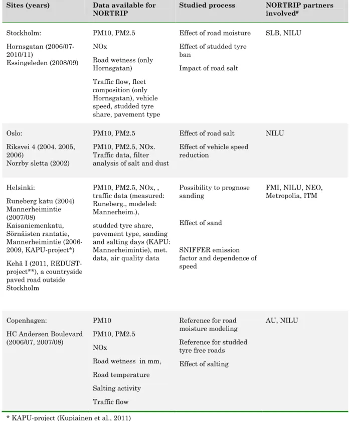
Table 3. Ambient measurement datasets used for NORTRIP model development and evaluation of the importance of different processes.
Sites (years) Data available for
NORTRIP Studied process NORTRIP partners involved# Stockholm: Hornsgatan (2006/07-2010/11) Essingeleden (2008/09) PM10, PM2.5 NOx
Road wetness (only Hornsgatan) Traffic flow, fleet composition (only Hornsgatan), vehicle speed, studded tyre share, pavement type
Effect of road moisture Effect of studded tyre ban
Impact of road salt
SLB, NILU Oslo: Riksvei 4 (2004. 2005, 2006) Norrby sletta (2002) PM10, PM2.5 PM10, PM2.5, NOx. Traffic data, filter analysis of salt and dust
Effect of road salt Effect of vehicle speed reduction NILU Helsinki: Runeberg katu (2004) Mannerheimintie (2007/08) Kaisaniemenkatu, Sörnäisten rantatie, Mannerheimintie (2006-2009, KAPU-project*) Kehä I (2011, REDUST-project**), a countryside paved road outside Stockholm
PM10, PM2.5, NOx, , traffic data (measured: Runeberg., modeled: Mannerheim.), studded tyre share, pavement type, sanding and salting days (KAPU: Mannerheimintie), met. data, air quality data
Possibility to prognose sanding
Effect of sand
SNIFFER emission factor and dependence of speed
FMI, NILU, NEO, Metropolia, ITM Copenhagen: HC Andersen Boulevard (2006/07, 2007/08) PM10 PM10, PM2.5 NOx Road wetness in mm, Road temperature Salting activity Traffic flow
Reference for road moisture modeling Reference for studded tyre free roads Effect of salting
AU, NILU
* KAPU-project (Kupiainen et al., 2011) **REDUST –project (www.redust.fi),
# ITM: Department of Applied Environmental Science, Atmospheric Science unit, Stockholm university, Sweden; NILU: The Norwegian Institute for Air Research, Kjeller, Norway; FMI:Finish Meteorological Institute, Helsinki, Finland; AU: Department of Environmental Science, Aarhus University, Denmark;
Metropolia:Helsinki Metropolia University of Applied Sciences, Finland; SLB:Environment and Health Administration, Stockholm, Sweden; VTI:Swedish National Road and Transport Research Institute, Linköping, Sweden; NEO:Nordic Envicon Oy, Helsinki, Finland.
6.1 Emission factors for road wear
Road wear due to the use of studded and non-studded tyres depend on the stone material of the pavement as well as the pavement type and the parameterizations of this is based on a number of studies in Sweden (Jacobson and Wågberg, 2007; Gustafsson et al., 2008), Norway (e g Snilsberg, 2008) and Finland (e g Kupiainen et al., 2005).
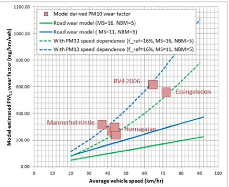
The road wear caused by studded tyres is based on the Swedish road wear model ((Jacobson and Wågberg, 2007) in which the road wear is calculated as a function of the maximum stone size, Nordic ball mill value and percentage stones >4 mm (for details see Berger and Sundvor, 2012). The PM10 fraction of the road wear depends on the Nordic ball mill value and maximum stone size as well as vehicle speed. The final default PM10 road wear fraction chosen (16%), based on model comparisons with PM10 concentrations recorded at traffic sites in Stockholm, Oslo and Helsinki as shown in Figure 2, is higher than reported by Gustafsson et al. (2008) but lower than reported by Snilsberg (2008).
Figure 2. Required PM10 wear factor necessary to obtain the annual mean concentrations for different datasets
(Mannerheimintie in Helsinki; RV4 in Oslo; Essingeleden and Hornsgatan in Stockholm). Also shown is the
road wear model estimates for PM10 wear factor based on the NORTRIP model as described in Denby and
Sundvor (2012). (MS=Maximum stone size, mm; NBM=Nordic ball mill value; f_ref=fraction PM10 of total road wear).
6.2 Emission factors based on mobile laboratory measurements
Data from two mobile laboratories have provided information on the potential suspension of road dust and its dependence on tyre and pavement type, vehicle speed and road conditions. In Finland the system is called Sniffer (e.g. Pirjola et al., 2004) and in Sweden it is called EMMA (Hussein et al., 2008). Both systems have been used in several projects and they provide measurements of traffic emissions under real driving conditions (Pirjola et al., 2009).
This section describes emission factors obtained using the Sniffer system. The Sniffer
instrumentation is set in a Volkswagen LT35 diesel van with a length 5585 mm, width 1933 mm, 2570 mm height with a maximum total weight of 3550 kg.
Sniffer measures resuspended dust concentration (PM10) behind its left rear tyre (Pirjola et al., 2009). Suspended dust is collected through a conical inlet with a surface area of 0.20 m x 0.22 m at 5 cm distance from the tyre into a vertical tube with a diameter of 0.1 m, 2000 L/min flow rate is produced by an electric engine on the roof. Mass concentration PM10 is monitored behind the
tyre by TEOM (Series 1400A, Rupprecht & Patashnick), recording a 30-s running average mass concentration every 10 s. The flow rate is 3 L/min. PM10 is also monitored by two DustTraks (TSI,
model 8530), one behind the tyre and the other above the front bumper at 0.7 m altitude, with a time resolution of 1 s. The test tyre was a friction tyre Nokian Hakkapeliitta CR 225/70/R15. Emission factors for Sniffer were determined by the upwind-downwind method (Etyemetzian et al., 2003). These measurements were conducted as a part of the REDUST (Best winter
maintenance practices to reduce respirable street dust in urban areas) -project on a street Suurmetsäntie in Helsinki in April 2011 when southern wind blew with a speed of 3 m s-1. In the
downwind side of the street a 10 m high tower was installed 3 m from the street lane. Three DustTraks were set at 1.9, 2.9 and 4.3 m altitudes. On the upwind side the fourth DustTrak was installed in the trailer (see details in Pirjola et al., 2012). Sniffer passed the tower with 50 km h-1.
According to the 10 successful passing experiments the measured concentrations were converted to emission factors following the TRAKER method (Gertler et al., 2006). Figure 3 presents the dependence of the Sniffer’s emission factor EF in mg/km (y-axis) on the resuspended PM10 in
g/m3, measured behind the tyre (also called Sniffer emission, see x-axis). For comparison, the
results from our earlier campaign in 2006 (Pirjola et al., 2007) are also included. The conversion equation for Sniffer is
EF = 18.46xPM100.55 (mg/km) (1)
This is valid when the resuspended PM10 concentration, measured behind the Sniffer’s tyre, is higher than 2000 g m-3. It should be noted that these values describe the conditions where the
street is dirty or very dirty (Kupiainen et al., 2011). Measurements are still missing for the PM10 concentrations < 2000 g m-3; awaiting more data, a linear approximation is assumed:
EF = 0.609xPM10 (mg/km) (2)
Figure 3. Emission factor (mg km-1) for Sniffer as a function of resuspended PM10 (g m-3) measured behind the Sniffer’s left rear tyre. The tyre is a friction tyre.
y = 18.463x0.5512 0 500 1000 1500 2000 2500 3000 0 2000 4000 6000 8000 Em is si on f ac tor ( m g/ km ) Sniffer-emission (µg/m3) Sniffer-Hernesaari-2006 Sniffer-Suurmetsäntie-2011 Vectra-Suurmetsäntie-2011 Power (Sniffer-Hernesaari-2006)
The dependence of Sniffer’s emission factor on the driving speed was studied based on two data sets. First, the resuspended PM10 concentrations were measured on a road situated about 30 km NE from Stockholm, Sweden, on 23 May 2007 (Pirjola et al., 2010). Visually on the 10 km way north three different parts of the road were easily separated due to different colors of the asphalt, all of the same quality (SMA with NBMI <9), but with different age. The sections were named as P1, P2 and P3 (see details in Pirjola et al., 2010). Steady driving speeds of 50, 65 and 80 km hr-1
were tested for a summer tyre, a non-studded winter tyre (friction tyre) and a studded winter tyre. All road sections were driven to north and south. The measured PM10 concentrations for the friction tyre were converted to the emission factors according to the equations (1)-(2) which are valid only for the friction tyre.
Figure 4 illustrates the dependence of the median emission factor over the different road sections P1N, P2S, and P3N. These sections were selected for this analysis so that the connecting unpaved road to the quarry disturbed the measurements as less as possible (see details in Pirjola et al., 2010). The dependence seems to be a power function where the exponent is unity or between 1 and 2. Note that only three driving speeds were used in this data set.
Figure 4. Dependence of Sniffer’s emission factor (eq 1 and 2) on driving speed based on the data set measured near Stockholm.
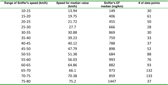
Second data set was obtained from measurements in Espoo, Finland, in March-May 2011 during the REDUST (Best winter maintenance practices to reduce respirable street dust in urban areas) -project. From the whole route we selected a part of the highway Kehä I (around 7 km) to obtain driving speeds from 10 km/h to 80 km/h (see details in Kupiainen et al., 2011). The variation of the 10 s TEOM data was high because many factors affect the resuspension. The data were classified according to the driving speed given in Table 4. The median values for the Sniffer’s emission factors were calculated based on the measured PM10 concentrations behind the left rear tyre and the equations (1)-(2).
Table 4. REDUST data for Sniffer.
Range of Sniffer's speed (km/h) Speed for median value
(km/h) Sniffer's EF median (mg/km) # of data points
10-15
13.94
149
30
15-20
19.75
406
61
20-25
21.72
455
50
25-30
27.7
666
28
30-35
30.88
869
30
35-40
39.23
759
33
40-45
40.12
788
37
45-50
47.79
898
52
50-55
51.38
684
88
55-60
56.03
993
76
60-65
64.86
882
93
65-70
66.1
973
132
70-75
70.38
859
133
75-80
75.2
1447
37
In this case the dependence of the Sniffer’s emission factor on the driving speed is almost linear as seen in Figure 5.
Figure 5. Dependence of Sniffer’s emission factor on driving speed based on the data set measured in Espoo. Median values with vertical bars indicating 25 and 75 percentiles.
It should be noted that the Sniffer’s emission factors discussed above concern only the case when the Sniffer vehicle has friction tyres (non-studded winter tyres). Because Sniffer is a van, its emission factors are presumably higher than the ones for passenger cars and lower than the ones for trucks. For example, Abu-Allaban et al. (2003) reported emission factors for resuspension of 224 (41-780) mg/km for light duty vehicles and 2247 (230-7800) mg/km for heady duty vehicles. There are also preliminary upwind-downwind measurements in Helsinki using a passenger car Opel Vectra, but the data has not been analysed so far.
Sniffer data has also been analyzed statistically against meteorological conditions and vehicle speed (Härkönen, et al., 2011a). Optimization of the results (Härkönen, et al., 2011b) suggests that the vehicle wake turbulence suspension and tyre-road surface suspension affect the emission factors differently depending on vehicle speed. The threshold speeds for the vehicle induced turbulence suspension and tyre-road surface suspension are about 30-40 km/h and 20 km/h, respectively, for the SNIFFER vehicle.
6.3 Wind induced suspension
The wind flow near the road surface is influenced by the turbulence or wake generated by the vehicles besides the normal meteorological wind flow than might be disturbed by buildings located on the sides of the road. The combination of wind and traffic generated turbulence will lead to the suspension of dust from the road surface into the air. On the “microscopic scale” the moving tyres are pressing air into the pores of the road surface at the front of the tyre and “sucking” air / dust out of the pores again behind the tyre. This complex interaction of turbulence at the tyre-road interface and the turbulence behind the vehicle will lead to a net suspension effect that depends on a number of parameters that are included in the NORTIP model describing the dust layer at the surface, moisture and vehicle parameters (vehicle speed, weight, tyres etc.). High ambient wind speeds might lead to suspension also in the absence of the vehicles. However this effect is less likely to play a significant role for the NORTRIP model for a number of reasons. The onset of significant wind induced suspension is observed for relatively high winds speeds of 7-10 m/s (Watson and Chow 2000; Vogt et al. 2011). Such high wind speeds are nor very frequent and are usually not the situations that are critical in terms of air pollution concentrations due to the high dilution in such situations. Moreover the vehicles are seldom absent in the roads considered here and movement of the vehicles (with 40-60 km/h about 11-17 m/s) and
corresponding turbulence is expected to be the dominating effect compared to pure wind induced turbulence.
6.4 Sandpaper effect
In the context of road dust emissions the sandpaper effect refers to a situation where traction sand grains are not only crushed under the tyres into small particles (even <10 µm) but they also increase the wear of the asphalt. This phenomenon was first observed in the road simulator tests described in Kupiainen et al. (2003) and further in Kupiainen et al (2005) and Kupiainen (2007). The basis for the sandpaper effect theory was the observation that in the sanded situation the contribution of the ambient PM10 particles originating from the pavement exceeded that observed
during the experiments with no sand on the pavement surface, which indicated that some additional process to e.g. stud wear must enhance the pavement wear resulting into more airborne emissions from the pavement. The only plausible explanation was that the sand grains interact with the pavement enhancing its wear. A further indication for the role of the sand grains was that the excess PM10 from the pavement was systematically observed to be higher with more resistant traction sand materials (Kupiainen 2007).
Figure 6 shows the contribution of the different source materials to the PM10 measured in the road simulator hall with studded and friction tyres and 300 g m-2 sand on the pavement surface
averaged over two measurements per tyre with different sanding materials. The overall PM10 level was higher with the studded tyre with more contribution from tyre induced pavement wear due to studs. The contribution from the pavement due to the sandpaper effect was higher with the friction tyre compared with the studded tyre but on the other hand the direct PM10 contribution from the sanding material was higher with the studded tyre. Different tread characteristics, sanding materials and the effect of studs may explain these differences in results, but more measurements are required to draw firm conclusions.
Figure 6. Contribution of the different source materials and the sandpaper effect to the PM10 measured in the road
simulator hall with friction and studded tyres and 300 g m-2 sand. The figure has been reproduced from the
information given in Kupiainen (2007).
The currently available measurement results on the sandpaper effect reviewed here represent the situation immediately after dispersion of sanding material on a dry bare pavement. The
measurements were conducted in a circular road simulator. Further studies should be conducted in road conditions to study the dynamics of the sandpaper effect and its general importance in the road dust problem.
Even though the NORTRIP model include a description of the additional abrasion of the road surface (sand paper effect) and the crushing of the sand and subsequent generation of
suspendable sand mass, there is insufficient information at the moment activate these processes in the model.
6.5 Importance of accurate surface moisture modeling
6.5.1 Road surface wetness measurements
Road surface moisture has been shown to be very critical for the variability of the PM10
concentrations (Norman and Johansson, 2006; Johansson et al., 2007)). Both direct and indirect PM10 emissions are substantially suppressed on wet road compared to dry. Worn material accumulates, increasing the depot during wet conditions. With studded tyres, road wear is larger on wet roads whereas tyre wear may be smaller if the road-tyre interaction is decreased due to the water film (the latter being irrespective of tyre type). Road surface moisture impacts on both the timing and the total emissions. Modeling both dust loading and moisture is essential for predicting both the variability and the absolute concentrations.
An illustration of the impact of road surface wetness is shown in Figure 7. The mean emission factor is several times higher during dry conditions compared to wet. During dry periods the emission factor is dominated by suspension and direct road wear emissions. During wet periods suspension of road dust is suppressed making exhaust and other wear more important. But it should be noted that the emission factor during “wet periods” in Figure 7 may also include suspension of road dust, since the definition of wet is based on the simple electric resistance between two wires on a very small part of the road, close to the measurement station.
Figure 7. Total PM10 emission factors (monthly averages based on measurements during 2006-2008) for Hornsgatan in Stockholm, derived from ambient air measurements during wet periods (blue line) and dry periods (black line).
There may be large variations in road surface wetness depending on where it is measured. On Hornsgatan there are three indicators at different locations; between lanes, in the middle of the street and between wheels (see Figure 8). Road wetness is measured as the electric resistance between two wires sticking up on the surface of the road.
Figure 8 shows the anti-correlation between incremental PM10 concentration (proportional to the emission factor) and road surface wetness. The measurements also indicates that the sensor located in the middle of the road (No. 1) is a less good indicator of the road wetness, this spot dries more slowly, likely due to less influence of traffic turbulence/heat and visibly more dust accumulated in the middle of the road; a large dust depot may store more water than if the surface is clean. This implies that it may be difficult to compare modeled road surface water with measurements on a small area.
Figure 8. PM10 increment (difference between urban background and street concentration) and road surface wetness measured at three locations in the surface.
0 1 2 3 4 5 6 0 200 400 600 800 1000 1200
Jan Feb Mar Apr Maj Jun Jul Aug Sep Okt Nov Dec
Ra ti o (d ry /w et ) P M1 0 emi ss io n fa ct o r mg /v eh ic le k
m) Wet periods Dry periods Ratio (dry/wet)
Delta PM10
Figure 9. Road surface wetness measurements using electrical wires on two streets in Stockholm. Hornsgatan runs in east-west and Sveavägen in north-south direction. Both have 24 meter high buildings on both sides of the street. Three sites on Hornsagatn (full line purple, red, orang) and two on Sveavägen (dotted lines grey and black).
Comparison of street wetness on different streets indicates different temporal variations in road wetness. Figure 9 indicates, indicating that the street direction may be important due to the shadowing effects of buildings. Shadowing is included in the NORTRIP model but it has not been shown to have a significant impact on the modeled concentrations for the data sets assessed.
6.5.2 Modeling of surface wetness
The NORTRIP model calculates road surface moisture based on the balance between sinks (evaporation, drainage, spray and freezing) and sources (rain, condensation and snow/ice melting), see Denby and Sundvor (2012).
A road sensor (IRS21, Signalbau Huber GmbH, Munich, Germany) has been installed in the road surface of HC Andersen Boulevard (Copenhagen) to measure road condition, temperature, salt content and amount of water (water film height).
Figure 10 shows a comparison of measured and calculated amount of water on the road surface on HC Andersen Boulevard for the year 2007-2008 with the inclusion of salt (including its impact on humidity) and without. The sensor is placed in the middle of the bus lane, located on the
outermost side of the road. In general, the model captures both the temporal variation and
absolute amount of water, but tends to overestimate the maximum moisture content. Without salt the surface tends to be drier.
In Figure 11 the surface wetness frequency is shown for both the years 2006-2007 and 2007-2008 and its sensitivity to wet salting, dry salting or no salting. For 2006-2007 salting improves the modeled frequency of surface wetness. For 2007-2008 there is overestimation with salt and underestimation without. Wet or dry salting makes little difference in both years.
Hornsgatan
Sveavägen
Figure 10. Comparison between modeled (blue) and measured (black) daily mean surface moisture on HC Anderssen Boulevard (Copenhagen) for the two available years of data, 2006-2007 (top) and 2007-2008 (bottom) .
Figure 11. Frequency of road wetness on HC Anderssen Boulevard (Copenhagen) for the two available years of data, 2006-2007 and 2007-2008. Shown is the impact of dry and wet salting on the modeled road wetness frequency.
In an effort to assess the potential error in modeled PM10 due to errors in the road surface moisture calculation, a comparison was made on Hornsgatan using the modeled and observed
Sep Oct Nov Dec Jan Feb Mar
0 0.2 0.4 0.6 0.8
HCAB 2006-2007: Road surface wetness
Surf ac e w et nes s (m m ) Date Road water depth
Observ ed water depth
Sep Oct Nov Dec Jan Feb Mar
0 0.2 0.4 0.6 0.8 Surf ac e s now (m m w .e. ) Date Road snow depth
Sep Oct Nov Dec Jan Feb Mar
0 0.2 0.4 0.6 0.8 1 R et ent ion fq Date Road Brake Observ ed
Sep Oct Nov Dec Jan Feb Mar
0 0.1 0.2 0.3 0.4 0.5 0.6 0.7
HCAB 2007-2008: Road surface wetness
Surf ac e w et nes s (m m ) Date Road water depth
Observ ed water depth
Sep Oct Nov Dec Jan Feb Mar
0 0.05 0.1 0.15 Surf ac e s now (m m w .e. ) Date Road snow depth
Sep Oct Nov Dec Jan Feb Mar
0 0.2 0.4 0.6 0.8 1 R et ent ion fq Date Road Brake Observ ed
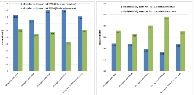
road wetness to determine surface retention. Using all 5 years of data (from July 1st – Dec 31st), the results are presented in Figure 12 and Figure 13 where the annual mean, the 90’th percentile, the correlation and the relative root mean square error (RMSE) are shown. Though the use of the moisture model clearly increases the RMSE and decreases correlation the annual mean and 90’th percentiles are less sensitive to the moisture modeling. This is only true if the moisture model is predicting a similar frequency of wet roads during the winter period. This is shown in Figure 14. In addition to the summary figures we also show the PM10 scatter plots for the year 2008-2009, daily and hourly, using both modeled and observed surface moisture in Figure 15.
Figure 12. Annual mean (left) and 90’th percentile (right) net PM10 daily mean concentrations for five years at
Hornsgatan. Shown are observed, modeled using observed moisture and modeled using modeled moisture.
Figure 13. Correlation (left) and relative RMSE (root mean square error) (right) of net PM10 daily mean concentrations for five years at Hornsgatan. Shown are modeled using observed moisture and modeled using modeled moisture.
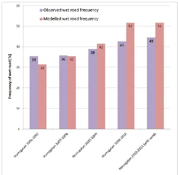
Figure 14. Road surface frequency of wet roads, observed and modeled, for Hornsgatan.
Figure 15. Comparison between observed and calculated PM10 using modeled moisture (left) and observed moisture
(right) for Hornsgatan 2008-2009. Shown are the daily means (top) and the hourly means (bottom).
0 20 40 60 80 100 120 140 160 0 20 40 60 80 100 120 140 160 Scatter plot PM10 + EP PM 1 0 obs erv ed c onc ent rat ion ( g/ m 3) PM10 modelled concentration (g/m 3 ) r2 = 0.58 RMSE = 19.5 (g/m3) OBS = 24.3 (g/m3) MOD = 24.0 (g/m3) a0 = 6.6 (g/m3) a1 = 0.74 0 20 40 60 80 100 120 140 160 0 20 40 60 80 100 120 140 160 Q-Q plot PM10 + EP PM 1 0 obs erv ed c onc ent rat ion ( g/ m 3) PM10 modelled concentration (g/m 3 ) 36th highest MOD = 53.5 (g/m3) 36th highest OBS = 58.9 (g/m3) Days > 50 g/m3 MOD= 43 Days > 50 g/m3 OBS = 50 0 5 10 15 20 25 30 0 5 10 15 20 25 30 Scatter plot PM2.5 + EP PM 2 .5 obs erv ed c onc ent rat ion ( g/ m 3) PM2.5 modelled concentration (g/m 3) r2 = 0.44 RMSE = 3.4 (g/m3) OBS = 6.6 (g/m3) MOD = 5.5 (g/m3) a0 = 0.8 (g/m3) a1 = 1.05 0 5 10 15 20 25 30 0 5 10 15 20 25 30 Q-Q plot PM2.5 + EP PM 2 .5 obs erv ed c onc ent rat ion ( g/ m 3) PM2.5 modelled concentration (g/m 3) 0 20 40 60 80 100 120 140 160 0 20 40 60 80 100 120 140 160 Scatter plot PM10 + EP PM 1 0 obs erv ed c onc ent rat ion ( g/ m 3) PM10 modelled concentration (g/m3) r2 = 0.90 RMSE = 9.1 (g/m3) OBS = 24.3 (g/m3) MOD = 24.3 (g/m3) a 0 = 1.6 (g/m 3) a 1 = 0.93 0 20 40 60 80 100 120 140 160 0 20 40 60 80 100 120 140 160 Q-Q plot PM10 + EP PM 1 0 obs erv ed c onc ent rat ion ( g/ m 3) PM10 modelled concentration (g/m3) 36th highest MOD = 60.6 (g/m3) 36th highest OBS = 58.9 (g/m3) Days > 50 g/m3 MOD= 44 Days > 50 g/m3 OBS = 50 0 5 10 15 20 25 30 0 5 10 15 20 25 30 Scatter plot PM2.5 + EP PM 2 .5 obs erv ed c onc ent rat ion ( g/ m 3) PM2.5 modelled concentration (g/m 3 ) r2 = 0.46 RMSE = 3.3 (g/m3) OBS = 6.6 (g/m3) MOD = 5.5 (g/m3) a0 = 0.6 (g/m3) a1 = 1.07 0 5 10 15 20 25 30 0 5 10 15 20 25 30 Q-Q plot PM2.5 + EP PM 2 .5 obs erv ed c onc ent rat ion ( g/ m 3) PM2.5 modelled concentration (g/m 3 ) 0 50 100 150 200 250 300 350 400 0 50 100 150 200 250 300 350 400 Scatter plot PM 10 + EP PM 1 0 obs erv ed c onc ent rat ion ( g/ m 3) PM10 modelled concentration (g/m3) r2 = 0.45 RMSE = 31.3 (g/m3) OBS = 25.8 (g/m3) MOD = 25.1 (g/m3) a0 = 8.6 (g/m3) a1 = 0.69 0 50 100 150 200 250 300 350 400 0 50 100 150 200 250 300 350 400 Q-Q plot PM 10 + EP PM 1 0 obs erv ed c onc ent rat ion ( g/ m 3) PM10 modelled concentration (g/m3) 0 10 20 30 40 50 60 70 80 0 10 20 30 40 50 60 70 80 Scatter plot PM2.5 + EP PM 2 .5 obs erv ed c onc ent rat ion ( g/ m 3) PM2.5 modelled concentration (g/m3) r2 = 0.37 RMSE = 5.3 (g/m3) OBS = 6.6 (g/m3) MOD = 5.9 (g/m3) a0 = 1.7 (g/m3) a1 = 0.84 0 10 20 30 40 50 60 70 80 0 10 20 30 40 50 60 70 80 Q-Q plot PM2.5 + EP PM 2 .5 obs erv ed c onc ent rat ion ( g/ m 3) PM2.5 modelled concentration (g/m3) 0 50 100 150 200 250 300 350 400 450 0 50 100 150 200 250 300 350 400 450 Scatter plot PM 10 + EP PM 1 0 obs erv ed c onc ent rat ion ( g/ m 3) PM10 modelled concentration (g/m3) r2 = 0.70 RMSE = 22.6 (g/m3) OBS = 25.8 (g/m3) MOD = 25.8 (g/m3) a0 = 4.9 (g/m3) a1 = 0.81 0 50 100 150 200 250 300 350 400 450 0 50 100 150 200 250 300 350 400 450 Q-Q plot PM 10 + EP PM 1 0 obs erv ed c onc ent rat ion ( g/ m 3) PM10 modelled concentration (g/m3) 0 10 20 30 40 50 60 70 80 0 10 20 30 40 50 60 70 80 Scatter plot PM2.5 + EP PM 2 .5 obs erv ed c onc ent rat ion ( g/ m 3) PM2.5 modelled concentration (g/m3) r2 = 0.39 RMSE = 5.2 (g/m3) OBS = 6.6 (g/m3) MOD = 5.9 (g/m3) a0 = 1.6 (g/m3) a1 = 0.85 0 10 20 30 40 50 60 70 80 0 10 20 30 40 50 60 70 80 Q-Q plot PM2.5 + EP PM 2 .5 obs erv ed c onc ent rat ion ( g/ m 3) PM2.5 modelled concentration (g/m3)
6.6 Importance of road salt
Road salt may contribute to the total mass of PM10 due to suspension from the road, especially
when the road surface is dry, but it may also affect the road moisture due to its effect on the evaporation and condensation of water vapor. As a result salt will add mass, but it will also reduce suspension by increasing surface wetness. The model has been applied to data from RV4 (Oslo) and Hornsgatan (Stockholm) as described below.
6.6.1 Application of the NORTRIP model to RV4, Oslo
An example is given using the Oslo RV4 data for 2005-2006. During this period the salting activities were not recorded and so the salting model was applied. Particular to this period was that, unlike previous years, the NaCl salt was mixed with MgCl2 as a dust inhibitor (higher
impact on the surface moisture humidity). The model was applied to the data in four ways:
1. Without salt (Figure 16)
2. With NaCl (20% solution) but with no humidity impact
3. With NaCl (20% solution) with the impact of salt on humidity and melt temperature
4. With 70% NaCl and 30% MgCl
2(20% solution) with the impact on the humidity and melt
temperature (Figure 17)
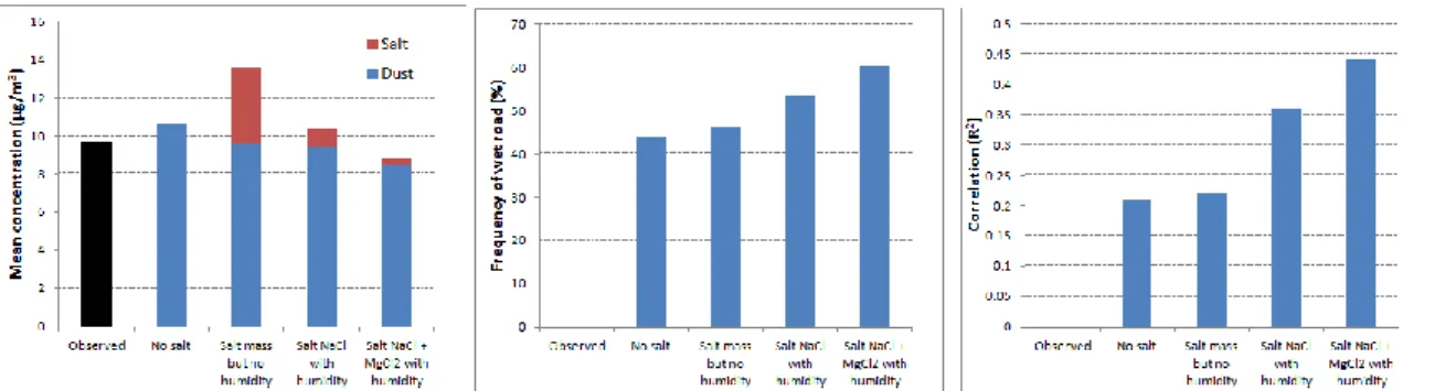
The results are summarized in Figure 18 where the mean concentrations of dust and salt, daily mean correlation and frequency of wet road resulting from the model are shown. The mean concentration of dust varies little with the different salting applications, since there are no removal processes other than suspension. However, since salt is efficiently removed by drainage and spray, retained salt will be removed from the road system much more efficiently than dust. The impact of salt on the moisture is best seen in the frequency of wet road which increases with the increased impact of salt humidity. The improvement in correlation is significant with the inclusion of the salt impact on humidity (from 0.21 with no salt to 0.45 for the mixed salt).
Figure 16. Model application to RV4 2005-2006 without salting using modeled surface moisture.
Sep Oct Nov Dec Jan Feb Mar Apr May
0 10 20 30 40 50 60 RV4 2005-2006: Concentrations PM 1 0 c onc ent rat ion ( g/ m 3) Date Observ ed Modelled salt Modelled dust Modelled sand Modelled+EP
Sep Oct Nov Dec Jan Feb Mar Apr May
0 2 4 6 8 10 12 14 PM 2 .5 c onc ent rat ion ( g/ m 3) Date Observ ed Exhaust Modelled+EP
Sep Oct Nov Dec Jan Feb Mar Apr May
0 100 200 300 400 500 600 700 NO X c onc ent rat ion ( g/ m 3) Date Observ ed Background Net
Figure 17. Model application to RV4 2005-2006 including salting (70% NaCl, 30% MgCl2) and its impact on humidity
using modeled surface moisture.
Figure 18. Summary of the model application to RV4 2005-2006 with different salting, using modeled surface moisture. Shown in the different columns are the results for no salt, salt in solution but no humidity impact, NaCl with
humidity impact and NaCl + MgCl2 with humidity impact. Left plot: Mean concentrations of dust and salt.
Centre plot: Frequency of wet road. Right plot: Correlation coefficient (R2) of the daily mean concentrations.
6.6.2 Application to Hornsgatan, Stockholm
During the winter 2010/2011 the exact timing and amount of salt, and sand, added to the road in Hornsgatan was recorded. There were 86 salting events in this period, with on average 60 kg/km/day over the 206 day period. For 2008/2009 there were no salting data available for comparison with modeled moisture. For the year 2008/2009 no salting or sanding data was available and salting was estimated using the salting model. The model was run in the following configurations:
1. Without salt (Year 2010-2011, Figure 19)
2. With reported NaCl (20% solution) but with no humidity impact
3. With estimated NaCl (20% solution) with the impact of salt on humidity and melt temperature
4. With reported NaCl (20% solution) with the impact of salt on humidity and melt temperature
(2010-2011 only)
5. With reported NaCl (20% solution) and using the observed surface moisture for retention
(Year 2010-2011, Figure 20)
The results are summarized in Figure 21 (2010-2011) and Figure 22 (2008-2009) where the mean concentrations of dust and salt and the daily mean correlation are shown. As in the Oslo case the mean concentration of dust varies little with the different salting applications. The impact of salt on the surface moisture is best seen in the correlation, since this reflects the timing of the road wetness. Using the observed surface moisture clearly provides the best model to estimate. It is worth noting that the estimated salting, using the salt model, gives much lower correlation than
Sep Oct Nov Dec Jan Feb Mar Apr May
0 10 20 30 40 50 60 RV4 2005-2006: Concentrations PM 1 0 c onc ent rat ion ( g/ m 3) Date Observ ed Modelled salt Modelled dust Modelled sand Modelled+EP
Sep Oct Nov Dec Jan Feb Mar Apr May
0 2 4 6 8 10 12 14 PM 2 .5 c onc ent rat ion ( g/ m 3) Date Observ ed Exhaust Modelled+EP
Sep Oct Nov Dec Jan Feb Mar Apr May
0 100 200 300 400 500 600 700 NO X c onc ent rat ion ( g/ m 3) Date Observ ed Background Net
using the reported salting, even though the number of salting events is almost exactly the same. In general salting has less impact on this year of data than on the Oslo dataset, but this varies from year to year and site to site., there were 49 salting events in this period (206 days) with on average 25 kg/km/day.
Figure 19. Model application to Hornsgatan 2010-2011 without salting using modeled surface moisture.
Figure 20. Model application to Hornsgatan 2010-2011 including reported salting using observed surface moisture.
Figure 21. Summary of the model application to Hornsgatan 2010-2011 with different salting, using modeled surface moisture. Shown in the different columns are the results for no salt, reported salt in solution but no humidity impact, estimated salt with humidity impact, reported salt with humidity impact and using the observed surface moisture. Left plot: Mean concentrations of dust and salt. Centre plot: 90’th percentile of the daily mean concentrations. Right plot: Correlation coefficient (R2) of the daily mean concentrations.
Jul Aug Sep Oct Nov Dec Jan Feb Mar Apr May Jun
0 50 100 150 200 Hornsgatan 2010-2011: Concentrations PM 1 0 c onc ent rat ion ( g/ m 3) Date Observ ed Modelled salt Modelled dust Modelled sand Modelled+EP
Jul Aug Sep Oct Nov Dec Jan Feb Mar Apr May Jun
0 5 10 15 PM 2 .5 c onc ent rat ion ( g/ m 3) Date Observ ed Exhaust Modelled+EP
Jul Aug Sep Oct Nov Dec Jan Feb Mar Apr May Jun
0 100 200 300 400 NO X c onc ent rat ion ( g/ m 3) Date Observ ed Background Net
Jul Aug Sep Oct Nov Dec Jan Feb Mar Apr May Jun
0 50 100 150 200 Hornsgatan 2010-2011: Concentrations PM 1 0 c onc ent rat ion ( g/ m 3) Date Observ ed Modelled salt Modelled dust Modelled sand Modelled+EP
Jul Aug Sep Oct Nov Dec Jan Feb Mar Apr May Jun
0 5 10 15 PM 2 .5 c onc ent rat ion ( g/ m 3) Date Observ ed Exhaust Modelled+EP
Jul Aug Sep Oct Nov Dec Jan Feb Mar Apr May Jun
0 100 200 300 400 NO X c onc ent rat ion ( g/ m 3) Date Observ ed Background Net
Figure 22. Summary of the model application to Hornsgatan 2008-2009 with different salting, using modeled surface moisture. Shown in the different columns are the results for i) no salt, ii) estimated salt in solution but no humidity impact, iii) estimated salt with humidity impact and iv) using the observed surface moisture. Left plot: Mean concentrations of dust and salt. Centre plot: 90’th percentile of the daily mean concentrations. Right plot: Correlation coefficient (R2) of the daily mean concentrations.
Important conclusions from these studies on salt and surface moisture are:
1. If salt is to be added in the model then it must include its impact on vapor pressure. Model
correlations are almost always substantially improved as a result of this. Salting without the
humidity impact will significantly increase the salt contribution.
2. Correlation is always highest when observed moisture is included. Only slight changes in the
surface moisture can have a large impact on the correlation. Even the difference between
estimated and reported salting can have a large impact on the correlation. For this observed
moisture should always be used when studying other model processes.
3. Annual means and percentiles do not differ significantly as a result of salting when the impact
of humidity is included. They do, however, tend to be reduced. This is because there are
currently no significant mechanisms for dust loss other than suspension in the model. If dust
was efficiently drained or sprayed from the road, or cleaning was carried out, then salting and
its enhanced retention effects would have a more significant impact on the concentrations.
6.7 Spray and splash
Splash is usually defined as the water thrown forwards and sidewards from the
tyre-/road-interface. It consists of relatively large droplets that are not caught by the air streams around the vehicle to any large extent. Also the sheets of slush thrown sidewards by traffic should be
regarded as belonging to the splash mechanism. Such mechanical transport in the immediate vicinity of the road can result in an uneven distribution of salt in the roadside environment. Spray, however, is thrown outwards by centrifugal action tangential from the tyre tread and a great proportion breaks down into small droplets with low sinking speed on hitting other parts of the vehicle. The spray is easily caught by the air streams and may be persistent in the air wake behind the vehicle for a long time. A truck wheel driving at a speed of 90 km/h on a wet road surface can lift as much as 400 litres of water per minute, 90 % of which falls back on the road surface, whereas the rest becomes spray (Sandberg, 1980; Weir et al., 1978).
6.8 Model sensitivity to sanding
There is only one data set available (Hornsgatan 2010-2011) where it is known when and how much sand has been applied to the surface. Size distribution measurements of traction sand used in Stockholm indicate a suspendable fraction (< 200 µm) of 6%. Sand with this fraction of
suspendable particles is applied in the model and the applied sand is allowed to be removed by suspension only, at the same rate as the wear particles. Applying the model in this way leads to a significant increase (factor of 2) in the modelled concentrations. Assuming that the size
distributions for sand are correct the inference is that sand is either less readily suspended than wear particles or that suspendable sand is more efficiently removed from the surface than wear particles. Information on this is not currently available.
The sensitivity of the model to the addition of sand is analysed for the Hornsgatan 2010-2011. The addition of 1 % suspendable sand slightly increased the correlation (by 0.01) and leads to an average contribution of around 2.7 µg/m3 compared to the contribution from road wear which is
7.8 µg/m3. In Figure 23 the impact of sanding for different suspendable fractions is shown for the
annual mean and the number of days above the limit value of 50 µg/m3. It should be noted that
during the winter 2010-2011 the amount of sand used in Stockholm and on Hornsgatan was much more than during an average year; normally Hornsgatan is not sanded or very seldom. In general, the contribution from sanding is expected to vary between years depending on the winter
conditions which define the need to use sanding for traction control (see section 6.9).
Given that the Hornsgatan datasets are fairly well modelled for most years without the use of sand (see Table 7 below), it appears that sand normally is not a significant contributor to the total emissions. The current analysis sets a range of 0.5 – 2% to the amount of suspendable material in the sand that is active for suspension. We choose a value of 1% in the model but clearly more information is required concerning this aspect.
Figure 23. Impact of traction sanding suspendable fraction (< 200 µm) on the annual mean and days above limit value (50 µg/m3) for the Hornsgatan 2010-2011 period. Also included are the observed values. Note all
concentrations are net concentrations, not included background.
6.9 An evaluation of predicting sanding and salting
The refined version of the SMHI model (Omstedt et al., 2005) applicable also in operational forecasting of air quality (Kauhaniemi et al., 2011) was used to study the possibility of predicting the sanding days and the influence of traction sanding to road dust suspension in Helsinki. The emission factors for suspension are modeled by considering the moisture content of the road surface and the particles origin from the wear of pavement and from the traction sand. In Finland, the sanding period, i.e., the time when traction sand and studded tyres are commonly used extends from October to May. The sand dust layer is increased once a day, when slippery