AI and Learning Systems
Industrial Applications and Future Directions
Edited by Konstantinos Kyprianidis
and Erik Dahlquist
and Erik Dahlquist
Over the last few years, interest in the industrial applications of AI and learning systems has surged. This book covers the recent developments and provides a broad
perspective of the key challenges that characterize the field of Industry 4.0 with a focus on applications of AI. The target audience for this book includes engineers involved in automation system design, operational planning, and decision support. Computer science practitioners and industrial automation platform developers will
also benefit from the timely and accurate information provided in this work. The book is organized into two main sections comprising 12 chapters overall:
• Digital Platforms and Learning Systems • Industrial Applications of AI Published in London, UK © 2021 IntechOpen © Artystarty / iStock ISBN 978-1-78985-877-8 A I a nd L ea rn in g S yste m s - I nd us tria l A pp lic atio ns a nd F utu re D ire cti on s
AI and Learning Systems
- Industrial Applications
and Future Directions
Edited by Konstantinos Kyprianidis
and Erik Dahlquist
Contributors
Weiwei Zhao, Tarek Hassan Mohamed, Gaber Salman, Hussein Abubakr Hussein, Mahmoud Hussein, Gaber Shabib, Andreas Roither-Voigt, Valdemar Lipenko, David Zelenay, Sebastian Nigl, Javad Khazaei, Dinh Hoa Nguyen, Moksadur Rahman, Örjan Larsson, Enislay Ramentol, Tomas Olsson, Shaibal Barua, Idelfonso B. R. Nogueira, Antonio Santos Sánchez, Maria. J. Regufe, Ana M. Ribeiro, Erik Dahlquist, Gladys Bonilla-Enriquez, Patricia Cano Olivos, José Luis Martínez Flores, Diana Sánchez Partida, Santiago Omar Caballero Morales, Karim Belmokhtar, Mauricio Higuita Cano, Jan Skvaril, Konstantinos Kyprianidis, Amare Desalegn Fentaye, Valentina Zaccaria, Ioanna Aslanidou
© The Editor(s) and the Author(s) 2021
The rights of the editor(s) and the author(s) have been asserted in accordance with the Copyright, Designs and Patents Act 1988. All rights to the book as a whole are reserved by INTECHOPEN LIMITED. The book as a whole (compilation) cannot be reproduced, distributed or used for commercial or non-commercial purposes without INTECHOPEN LIMITED’s written permission. Enquiries concerning the use of the book should be directed to INTECHOPEN LIMITED rights and permissions department (permissions@intechopen.com).
Violations are liable to prosecution under the governing Copyright Law.
Individual chapters of this publication are distributed under the terms of the Creative Commons Attribution - NonCommercial 4.0 International which permits use, distribution and reproduction of the individual chapters for non-commercial purposes, provided the original author(s) and source publication are appropriately acknowledged. More details and guidelines concerning content reuse and adaptation can be found at http://www.intechopen.com/copyright-policy.html.
Notice
Statements and opinions expressed in the chapters are these of the individual contributors and not necessarily those of the editors or publisher. No responsibility is accepted for the accuracy of information contained in the published chapters. The publisher assumes no responsibility for any damage or injury to persons or property arising out of the use of any materials, instructions, methods or ideas contained in the book.
First published in London, United Kingdom, 2021 by IntechOpen
IntechOpen is the global imprint of INTECHOPEN LIMITED, registered in England and Wales, registration number: 11086078, 5 Princes Gate Court, London, SW7 2QJ, United Kingdom Printed in Croatia
British Library Cataloguing-in-Publication Data
A catalogue record for this book is available from the British Library Additional hard and PDF copies can be obtained from orders@intechopen.com AI and Learning Systems - Industrial Applications and Future Directions Edited by Konstantinos Kyprianidis and Erik Dahlquist
p. cm.
Print ISBN 978-1-78985-877-8 Online ISBN 978-1-78985-878-5 eBook (PDF) ISBN 978-1-83968-601-6
An electronic version of this book is freely available, thanks to the support of libraries working with Knowledge Unlatched. KU is a collaborative initiative designed to make high quality books Open Access for the public good. More information about the initiative and links to the Open Access version can be found at www.knowledgeunlatched.org
Selection of our books indexed in the Book Citation Index in Web of Science™ Core Collection (BKCI)
Interested in publishing with us?
Contact book.department@intechopen.com
Numbers displayed above are based on latest data collected. For more information visit www.intechopen.com
5,200+
Open access books available
156
Countries delivered to Contributors from top 500 universities
12.2%
Our authors are among the
Top 1%
most cited scientists
128,000+
International authors and editors
150M+
DownloadsWe are IntechOpen,
the world’s leading publisher of
Open Access books
Built by scientists, for scientists
BOOK CITATION
INDEX CLAR
IVATE ANALYTIC
S
Meet the editors
Prof. Konstantinos G. Kyprianidis is a Full Professor in Energy Engineering within the Future Energy Center at Mälardalen University in Sweden. He leads the SOFIA research group (Simu-lation and Optimization for Future Industrial Applications) and is the Head of Research Education for Energy & Environmental Engineering. He has been the Principal Investigator of a large number of national and international research projects relat-ed to automation in the energy and process industry. Among others, he has been the Chief Engineer for the 5.75mEuro project FUDIPO funded by the European Commission. Prior to coming to MDH, he worked for Rolls-Royce plc in the United Kingdom. He has co-authored over 140 peer-reviewed publications and current-ly supervises 15 doctoral candidates and is the Chair of the ASME/IGTI Aircraft Engine Committee.
Prof. Erik Dahlquist is a Senior Professor of Energy Technolo-gy and was the former Research Director of the Future EnerTechnolo-gy Center from 2000 to 2017 at Mälardalen University in Sweden. Among many other projects, he is the Project Coordinator Engi-neer for the 5.75mEuro project FUDIPO funded by the European Commission. Prior to joining MDH, he worked for 28 years at ABB Sweden in various senior technical and management roles. He has co-authored over 300 peer-reviewed publications and currently supervises 10 doctoral candidates.
Preface XI
Acknowledgment V
Section 1
Digital Platforms and Learning Systems 1
Chapter 1 3
AI Overview: Methods and Structures
by Erik Dahlquist, Moksadur Rahman, Jan Skvaril and Konstantinos Kyprianidis
Chapter 2 25
A Framework for Learning System for Complex Industrial Processes
by Moksadur Rahman, Amare Desalegn Fentaye, Valentina Zaccaria, Ioanna Aslanidou, Erik Dahlquist and Konstantinos Kyprianidis
Chapter 3 55
AI & Digital Platforms: The Market [Part 1]
by Örjan Larsson
Chapter 4 81
AI & Digital Platforms: The Technology [Part 2]
by Örjan Larsson
Chapter 5 105
Artificial Intelligence and ISO 26000 (Guidance on Social Responsibility)
by Weiwei Zhao
Chapter 6 117
Operationalizing Heterogeneous Data-Driven Process Models for Various Industrial Sectors through Microservice-Oriented Cloud-Based Architecture
by Valdemar Lipenko, Sebastian Nigl, Andreas Roither-Voigt and Zelenay David
Section 2
Industrial Applications of AI 137
Chapter 7 139
Machine Learning Models for Industrial Applications
Preface XIII
Acknowledgment XV
Section 1
Digital Platforms and Learning Systems 1
Chapter 1 3
AI Overview: Methods and Structures
by Erik Dahlquist, Moksadur Rahman, Jan Skvaril and Konstantinos Kyprianidis
Chapter 2 25
A Framework for Learning System for Complex Industrial Processes
by Moksadur Rahman, Amare Desalegn Fentaye, Valentina Zaccaria, Ioanna Aslanidou, Erik Dahlquist and Konstantinos Kyprianidis
Chapter 3 55
AI & Digital Platforms: The Market [Part 1]
by Örjan Larsson
Chapter 4 81
AI & Digital Platforms: The Technology [Part 2]
by Örjan Larsson
Chapter 5 105
Artificial Intelligence and ISO 26000 (Guidance on Social Responsibility)
by Weiwei Zhao
Chapter 6 117
Operationalizing Heterogeneous Data-Driven Process Models for Various Industrial Sectors through Microservice-Oriented Cloud-Based Architecture
by Valdemar Lipenko, Sebastian Nigl, Andreas Roither-Voigt and Zelenay David
Section 2
Industrial Applications of AI 137
Chapter 7 139
Machine Learning Models for Industrial Applications
Consensus Control of Distributed Battery Energy Storage Devices in Smart Grids
by Javad Khazaei and Dinh Hoa Nguyen
Chapter 9 175
Power Flow Management Algorithm for a Remote Microgrid Based on Artificial Intelligence Techniques
by Karim Belmokhtar and Mauricio Higuita Cano
Chapter 10 201
Adaptive Load Frequency Control in Power Systems Using Optimization Techniques
by Tarek Hassan Mohamed, Hussein Abubakr, Mahmoud M. Hussein and Gaber S. Salman
Chapter 11 217
Modeling the Hidden Risk of Polyethylene Contaminants within the Supply Chain
by Gladys Bonilla-Enríquez, Patricia Cano-Olivos, José-Luis Martínez-Flores, Diana Sánchez-Partida and Santiago-Omar Caballero-Morales
Chapter 12 231
Sustainable Energy Management of Institutional Buildings through Load Prediction Models: Review and Case Study
by Antonio Santos Sánchez, Maria João Regufe, Ana Mafalda Ribeiro and Idelfonso B.R. Nogueira
Preface
Artificial Intelligence (AI) was a “hot” research topic within industrial automation in the early 1980s with developments focused on methods for diagnostics, simula-tion, model adaptasimula-tion, and optimal control. Artificial neural networks were used extensively at the time within a number of industrial automation applications. Issues included robustness and available computational capacity for online and real-time applications.
It took the best part of the next 3 decades to develop practical solutions to these shortcomings, and gradually bring the technology to the level of “intelligence” required to leverage benefits compared to traditional approaches. As a result, interest in the industrial applications of AI and learning systems have surged anew over the last few years. Several powerful methods and digital platforms have been developed during the past decade, and the number of industrial applications has been growing exponentially. This is rapidly changing the way of doing things within the process and energy industry, as well as other industrial sectors.
This book covers recent developments and provides a broad perspective of the key challenges that characterize the field of Industry 4.0 with a focus on applications of AI. The target audience for this book includes engineers involved in automation system design, operational planning, and decision support. Computer science practitioners and industrial automation platform developers will also benefit from the timely and accurate information provided in this work.
The book is organized into two main sections comprising 12 chapters overall: (i) Digital Platforms and Learning Systems
(ii) Industrial Applications of AI
The academic editor is indebted to all his colleagues from across the world that contributed to this book with their latest research, to Prof. Erik Dahlquist for joining this effort as co-editor, to several automation experts who volunteered as reviewers, as well as to IntechOpen Publishers for giving me the opportunity to work on this book and its members of staff for their constant support during its preparation.
Konstantinos G. Kyprianidis and Erik Dahlquist
Professor, Mälardalen University, Västerås, Sweden
Acknowledgments
This project has received funding from the European Union’s Horizon 2020 research and innovation programme under grant agreement No 723523.
Acknowledgments
This project has received funding from the European Union’s Horizon 2020 research and innovation programme under grant agreement No 723523.
Digital Platforms
and Learning Systems
Digital Platforms
and Learning Systems
AI Overview: Methods and
Structures
Erik Dahlquist, Moksadur Rahman, Jan Skvaril
and Konstantinos Kyprianidis
Abstract
This paper presents an overview of different methods used in what is normally called AI-methods today. The methods have been there for many years, but now have built a platform of methods complementing each other and forming a cluster of tools to be used to build “learning systems”. Physical and statistical models are used together and complemented with data cleaning and sorting. Models are then used for many different applications like output prediction, soft sensors, fault detection, diagnostics, decision support, classifications, process optimization, model predictive control, maintenance on demand and production planning. In this chapter we try to give an overview of a number of methods, and how they can be utilized in process industry applications.
Keywords: process industry, artificial intelligence (AI), learning system, soft sensors, machine learning
1. Introduction
During the 80th AI was a hot topic both in the academia and industries. Many researchers were working a lot with development of methods for diagnostics, sim-ulation and adaptation of models. Artificial Neural Networks (ANN) were being implemented in real applications such as e.g. soft sensors to predict NOx concen-tration in exhaust gas from power plants. Still there was quite some “over-selling” and the enthusiasm for AI in the future was assumed to be useful tomorrow. But it took much longer to get the systems robust enough to be used and fast enough to be applicable in on-line applications. After year 2000, systems started to reach a more mature state and we got IBMs Watson, that could beat the Jeopardy master. Later the Google tool could beat the “Go-master”, a very complex Chinese game. This has changed the perception of AI. It is still similar type of tools as were developed during the 80th, but now they were refined a lot and hardwires has been developed dramatically. This has given us a much more positive perception of what can be done, and a lot is now being implemented. Still there is a risk for over-selling, as the tools are normally not that “intelligent” as we normally think of when we talk about Intelligence. But we are closing the gap day by day.
Concerning use of AI in process industry, we cannot just take the tools and hope they will fix everything. It is still important to identify “what is the problem to solve”? With Jeopardy the goal is to be good at Jeopardy, but what is the goal in process industry? It should be to increase production, reduce process variations,
implement maintenance on-demand and give operator support. It also means to coordinate and optimize production lines as well as complete plants and later on complete corporations. It also means to adapt to changing customer demands, support in development of new products with production lines as well as handle new business models. These different functions demand quite different tools and thus we will not use only one but several. Often Machine learning is considered being “the tool”, but often there is not data available to implement ML, especially not when starting a new production line. To implement new tools, it is also very important to pre-treat data. You have to sort data in “normal variations” or “anom-alies”. You may need to filter data with moving windows, but in different time perspectives. We need to do data reconciliation to handle drifting sensors. And you need to integrate all levels from orders to production planning down to coordinated and optimized production. In this chapter we will discuss a number of different methods as well as discuss integration between the different levels. Over the years many researchers have investigated different AI techniques for different process industrial application. A comprehensive review on different AI models applied in energy systems can be found in [1]. Applications of different AI tools based on simulation models in pulp and paper industry has been presented by researchers including Dahlquist [2–5]. Applications in power plants have been presented in many articles including Karlsson et al. [6–8]. In Karlsson et al. [9] a general discussion is made on how to make better use of data including pretreatment of data. Adaptation to degeneration in process models by time is discussed in Karlsson et al. [7]. [10] conducted an extensive review on different AI based soft sensors in process industries. 1.1 Similarities between AI and how the brain works
The mathematicians developing especially ANN have been looking a lot on how the brain works. In Figure 1 we see a principal picture of a human.
Running in a forest: The brain stores many different factors locally by “tuning many soft sensors”. During the night strength of connections are enhanced for the most important functions, while other less important connections are eliminated. Some information is used for direct control. Others is stored for use later on.
If it is rainy when you run there is a general feeling that “this was not so nice”. Everything else happening in the forest then will be “colored” by this in your mem-ory, aside of concrete thing like if you meet someone, like a friend, during the run.
Figure 1.
How a human handle input from the surrounding.
Short term memory: Dorsolateral prefrontal cortex controls information stream from sensors. Skull lobe is for attention. Ventrolateral prefrontal cortex sort infor-mation into useful or not useful info. Supplementary motor area (SMA) repeat new memories all over.
Long term memory: Hippocampus and nearby areas in medial temple globe are essential for long term memory. Facts are stored. Small brain and basial ganglia contain procedural memory, like how to bike or swim.
A human may have approximately 120 billion nerve cells. Each connect to hundreds of other cells. Some connections enhance while other decrease signals. Very complex interactions where connections are established and broken continu-ously. No exact values or memories exist for control, but diffuse input give diffuse output, but with different feed-back mechanisms. The Swedish Nobel Prize winner Arvid Carlsson [11] found out the mechanism of how signals are transferred from the dendrite of one cell to the axon of the next, where complex feed-back mecha-nisms enhance a connection and thereby also enforced a memory by changing the easiness of transferring new signals. He explored how dopamine works as a signal substance, which we now know is of highest importance in the brain. By back-propagation in ANN we try to simulate this mechanism (Figure 2).
Input to the brain is sorted in Amygdala and hippocampus. Signals are sent to different part of the brain Here different signals are enhanced or decreased depending on previous experiences in many different “soft sensors”, built up with tuning of Ca-channels working as parameters in a polynom. “= enhancement fac-tors”. The situation is triggering memory build up. All control is “diffuse” using many different “diffuse” measurements. Different individuals have different sensi-tivity and number of different sensors like sense for bitterness, sugar, pain etc. Soft sensors get input and react with output to other soft sensors. Signals are sent to direct different biochemical processes like when fear - increase production of Adrenalin and Cortisone. This in turn is affecting many other hormones and pro-teins etc. Also, microbiome in the stomach and skin send input to the brain on how these organs perform. When you run, the body feel good and e.g. endorphins are produced enhancing performance of stomach, muscles etc. Serotonin levels,
Figure 2.
gibberellins, insulin, cortisone etc. are interacting and tuning each other, but with influence “from the side” by other sensor inputs. The brain is interacting with all this. This is also the basic concept to mimic in “deep learning”.
If we try to transfer this picture into a control system, it can look like below in Figure 3.
We start with sorting out “outliers” in pre-processing. This is what the brain does with information from the eye etc. The outliers can be used for anomaly detection. This is principally what is done in Amygdala. We then compare pre-dictions from simulators and soft- sensors to measurements. We trend differences developed by time. Refined data are used for model building and adaptation of models. The models are used for soft sensors, diagnostics, control etc. We also make conclusions in decision a tree from previous experience and identify optimal action to take in different time perspectives. In the brain this is done by utilizing previous experience in a way where we try to “make sense”. This means that we replace missing data with what is reasonable. In our computer system we do this by data-reconciliation using e.g. solving an equation system of physical models to get a best fit. We then take actions by control of many different functions more. In the body, this means e.g. control of sugar content in the blood, release of adrenalin to meet threats or melatonin to make you tired and go to sleep. We learn buy tuning soft sensors and decision trees with the new information just as the brain does, but where the brain is very much more complex than what we can handle today. 1.2 Market aspects
IndTech’s market, i.e. Products and systems for industrial digitization and auto-mation in the world are worth around USD 340 billion in 2016/2017 and have an average growth rate of 7–8 percent. The area can be divided into two parts: IT (industrial IT) and OT (operational technology). The share that can be categorized into industrial IT is about USD 110–120 billion. The remaining USD 220 billion is operational technology for the factory floors and in the field. It, in turn, is tradi-tionally divided into discrete automation (about 45 percent) and process automa-tion (about 55%). OT includes various types of industrial control systems (ICS) and field equipment such as instrumentation, analysis, drive systems, motors, robots and similar.
For the future of AI, we can see that this comes deeply into all these industrial market segments, but also far beyond as not only for industrial applications.
Figure 3.
Principal diagram of signal processing in a “learning system”.
The tools thus will be developed for one application, but then will be used also for other applications most probable.
2. Different AI methods
There are many different methods developed. Some of them are very similar or aim to solve the same type of problems. If we look at Machine learning (ML), we have e.g. Regression. Artificial Neural Networks (ANN), Support Vector Machines (SVM), Principal Component Analysis (PCA), Partial Least Square regression (PLS) and etc. They both aim to sort different variables into group that correlate to different properties or faults.
PLS and ANN, both are very useful to create soft sensors. Deep learning is a sophisticated version of the ANN, but with the goal to produce models that can do much more than just be a soft sensor, which predicts one or more qualities. Exam-ples of soft sensors is to predict strength properties of paper from e.g. NIR data and process variable values in paper machines, amount of different kind of plastics in Waste combustion plants or protein content in cereals in agriculture from NIR spectra. The deep learning on the other hand can be used to teach a robot to pick out machine components that are scrapped from a conveyor belt for instance. This then includes image pattern analysis from camera monitoring of the parts passing.
A selection of different tools is listed in Table 1. 2.1 Machine learning methods
Machine learning methods principally use a lot of process data measured pref-erably on-line, and identify correlation models from the data, which can be used for different purposes like soft sensors, anomaly detection and others.
There are several different machine learning methods. Some are correlating a specific property to process data. Reinforcement learning is described in e.g. Gattami Ather [12]. It is used in problems where actions (decisions) have to be made and each action (decision) affects future states of the system. Success is measured by a scalar reward signal and proceed to maximize reward (or minimize cost) where no system model is available. One example of this technique is deep reinforcement learning which was used in AlphaGo that defeated the World Champion in Go. Here a Q function is approximated with a deep neural network. Minimizing the loss function with respect to the neural network weights w is made as given below
l ¼ r s, aðð Þ þ δsupQ ´s, ´a, w�ð Þ � Q s, a, wð ÞÞ2 (1)
• Gaussian Process Regression (GPR)
• Partial Least Square (PLS) Regression
• Principal Component Analysis (PCA)
• Artificial Neural Networks (ANN)
• Support Vector Machines (SVM)
• Gray box models
• Physical models, MPC – model predictive control
• Bayesian networks (BN)
• Gaussian Mixture Model (GMM)
• Reinforcement Learning
• Google algorithm – search engines
Table 1.
gibberellins, insulin, cortisone etc. are interacting and tuning each other, but with influence “from the side” by other sensor inputs. The brain is interacting with all this. This is also the basic concept to mimic in “deep learning”.
If we try to transfer this picture into a control system, it can look like below in Figure 3.
We start with sorting out “outliers” in pre-processing. This is what the brain does with information from the eye etc. The outliers can be used for anomaly detection. This is principally what is done in Amygdala. We then compare pre-dictions from simulators and soft- sensors to measurements. We trend differences developed by time. Refined data are used for model building and adaptation of models. The models are used for soft sensors, diagnostics, control etc. We also make conclusions in decision a tree from previous experience and identify optimal action to take in different time perspectives. In the brain this is done by utilizing previous experience in a way where we try to “make sense”. This means that we replace missing data with what is reasonable. In our computer system we do this by data-reconciliation using e.g. solving an equation system of physical models to get a best fit. We then take actions by control of many different functions more. In the body, this means e.g. control of sugar content in the blood, release of adrenalin to meet threats or melatonin to make you tired and go to sleep. We learn buy tuning soft sensors and decision trees with the new information just as the brain does, but where the brain is very much more complex than what we can handle today. 1.2 Market aspects
IndTech’s market, i.e. Products and systems for industrial digitization and auto-mation in the world are worth around USD 340 billion in 2016/2017 and have an average growth rate of 7–8 percent. The area can be divided into two parts: IT (industrial IT) and OT (operational technology). The share that can be categorized into industrial IT is about USD 110–120 billion. The remaining USD 220 billion is operational technology for the factory floors and in the field. It, in turn, is tradi-tionally divided into discrete automation (about 45 percent) and process automa-tion (about 55%). OT includes various types of industrial control systems (ICS) and field equipment such as instrumentation, analysis, drive systems, motors, robots and similar.
For the future of AI, we can see that this comes deeply into all these industrial market segments, but also far beyond as not only for industrial applications.
Figure 3.
Principal diagram of signal processing in a “learning system”.
The tools thus will be developed for one application, but then will be used also for other applications most probable.
2. Different AI methods
There are many different methods developed. Some of them are very similar or aim to solve the same type of problems. If we look at Machine learning (ML), we have e.g. Regression. Artificial Neural Networks (ANN), Support Vector Machines (SVM), Principal Component Analysis (PCA), Partial Least Square regression (PLS) and etc. They both aim to sort different variables into group that correlate to different properties or faults.
PLS and ANN, both are very useful to create soft sensors. Deep learning is a sophisticated version of the ANN, but with the goal to produce models that can do much more than just be a soft sensor, which predicts one or more qualities. Exam-ples of soft sensors is to predict strength properties of paper from e.g. NIR data and process variable values in paper machines, amount of different kind of plastics in Waste combustion plants or protein content in cereals in agriculture from NIR spectra. The deep learning on the other hand can be used to teach a robot to pick out machine components that are scrapped from a conveyor belt for instance. This then includes image pattern analysis from camera monitoring of the parts passing.
A selection of different tools is listed in Table 1. 2.1 Machine learning methods
Machine learning methods principally use a lot of process data measured pref-erably on-line, and identify correlation models from the data, which can be used for different purposes like soft sensors, anomaly detection and others.
There are several different machine learning methods. Some are correlating a specific property to process data. Reinforcement learning is described in e.g. Gattami Ather [12]. It is used in problems where actions (decisions) have to be made and each action (decision) affects future states of the system. Success is measured by a scalar reward signal and proceed to maximize reward (or minimize cost) where no system model is available. One example of this technique is deep reinforcement learning which was used in AlphaGo that defeated the World Champion in Go. Here a Q function is approximated with a deep neural network. Minimizing the loss function with respect to the neural network weights w is made as given below
l ¼ r s, að ð Þ þ δsupQ ´s, ´a, w�ð Þ � Q s, a, wð ÞÞ2 (1)
• Gaussian Process Regression (GPR)
• Partial Least Square (PLS) Regression
• Principal Component Analysis (PCA)
• Artificial Neural Networks (ANN)
• Support Vector Machines (SVM)
• Gray box models
• Physical models, MPC – model predictive control
• Bayesian networks (BN)
• Gaussian Mixture Model (GMM)
• Reinforcement Learning
• Google algorithm – search engines
Table 1.
If the system is deterministic the model is given by
Skþ1¼ fkðsk, akÞ (2)
If the system is stochastic the model is given by
P sðkþ1jsk, akÞ (3)
fkðsk, akÞ is a scalar valued reward.
In Werbos Paul: A Menu of Design for reinforcement learning over time [13] reinforcement methods are described more generally.
2.2 Soft sensors
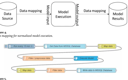
It is interesting to create soft sensors by creating models correlating process measurements on-line to quality measurements from samples analyzed at lab. The soft sensor then can be used to predict the quality property on-line from feeding the on-line measurements into the soft sensor model. There are several different methods for the regression, and a number of alternatives are given in Figure 4 below.
In Figure 5 we see how the data flow can look like for data collection, data pre-processing, model building and model validation. Here NIR measurements are correlated to properties like lignin content.
Soft sensors also can be built with other methods like using ANN, Artificial Neural nets. There are advantages and disadvantages with the different methods, but also commonalities. You need good data for building the models. This means that data need to be spread out in the value space in a good way. If we only have
“white noise” the models will be unusable. We need to vary all variables in a
systematic way to get useful data for model building. 2.3 Gaussian process regression model
Gaussian Process Regression takes more memory but gives better regression models than many other methods like (Nonlinear) System Identification, Neural Networks and Adaptive learning models. Can also be Combine with physics-based models. The method is presented in e.g. Fredrik et al. [14]. In Figure 6 we see a first attempt to predict kappa number of pulps after a digester for two different wood
Figure 4.
A number of methods that can be used to develop soft sensor models from process data.
types, hardwood and soft wood. The training data fits quite well, while the pre-dictions are less good. By using more data and fine-tune the estimation of residence time in the reactor the prediction power became significantly better. It went from
R2= 54 to R2> 90.
2.4 Artificial neural nets, ANN
Artificial neural nets try to mimic the brain. In a simple way we can use the equation below to show how it is calculated:
Figure 5.
Data flow for building and verification of soft sensors.
Figure 6.
If the system is deterministic the model is given by
Skþ1¼ fkðsk, akÞ (2)
If the system is stochastic the model is given by
P sðkþ1jsk, akÞ (3)
fkðsk, akÞ is a scalar valued reward.
In Werbos Paul: A Menu of Design for reinforcement learning over time [13] reinforcement methods are described more generally.
2.2 Soft sensors
It is interesting to create soft sensors by creating models correlating process measurements on-line to quality measurements from samples analyzed at lab. The soft sensor then can be used to predict the quality property on-line from feeding the on-line measurements into the soft sensor model. There are several different methods for the regression, and a number of alternatives are given in Figure 4 below.
In Figure 5 we see how the data flow can look like for data collection, data pre-processing, model building and model validation. Here NIR measurements are correlated to properties like lignin content.
Soft sensors also can be built with other methods like using ANN, Artificial Neural nets. There are advantages and disadvantages with the different methods, but also commonalities. You need good data for building the models. This means that data need to be spread out in the value space in a good way. If we only have
“white noise” the models will be unusable. We need to vary all variables in a
systematic way to get useful data for model building. 2.3 Gaussian process regression model
Gaussian Process Regression takes more memory but gives better regression models than many other methods like (Nonlinear) System Identification, Neural Networks and Adaptive learning models. Can also be Combine with physics-based models. The method is presented in e.g. Fredrik et al. [14]. In Figure 6 we see a first attempt to predict kappa number of pulps after a digester for two different wood
Figure 4.
A number of methods that can be used to develop soft sensor models from process data.
types, hardwood and soft wood. The training data fits quite well, while the pre-dictions are less good. By using more data and fine-tune the estimation of residence time in the reactor the prediction power became significantly better. It went from
R2= 54 to R2> 90.
2.4 Artificial neural nets, ANN
Artificial neural nets try to mimic the brain. In a simple way we can use the equation below to show how it is calculated:
Figure 5.
Data flow for building and verification of soft sensors.
Figure 6.
^
y tjθð Þ ¼ a1∗ κ γð 1þ β11φ1ð Þ þ βt 21φ2ð ÞtÞ þ α2∗ κ γð 2þ β12φ1ð Þ þ βt 22φ2ð ÞtÞ (4)
In Figure 7 we see three input variables to the left. Each variable is multiplied with a weight factor towards the two summa-nodes, where the products are sum-marized. Next these values can be treated to pass a threshold or only be passed on
and multiplied with a second constantαi. The two products are summarized again,
and we get a prediction of the value of a wanted property. When you build the net, you look at the difference between the measured and the predicted value and adjust the weight factors until you get a good fit. When you have been testing one set of input variables you go to the next and proceed for all data you have and try to get a fit that is the best for all input variables together. This is a simple net with only one
“hidden layer”, but you can have much more complex versions with many variables
and many layers. If you have many layers the problem though can be that you get a good fit for the training data but it may also give risk for “over-fitting”, which means less stable predictions.
An example of a first commercial application of ANN was for prediction of NOx in power plants. In Figure 8 below we see a regression for the power boiler number four in Vasteras.
2.5 PLS, partial least square regression and factorial design of experiments PLS is very popular to use for making prediction models after performing facto-rial designs of experiments. The basic idea is to start with a linear regression for a
line, y ¼ a þ b ∗ x, and adding non-linearity by þc ∗ x2and if there are more than
one variable the interaction between variable 1 and 2 by d∗ x1∗ x2. The polynomial
for a property like a strength property of a paper then becomes
y ¼ A þ B ∗ x1þ C ∗ x2þ D ∗ x12þ E ∗ x22þ F ∗ x1∗x2 (5)
Here A-F are constants you get from fitting the experimental data to the model. If we use factorial design, it means that we try to expand the prediction space as much as possible within given borders. This means that we shall have a good distribution of experimental data in all parts of the space, and not only close to origo or in one part of the space. This means for example that you shall not make
correlation for one variable at a time but vary all variables in a systematic way. In Ferreira et al. [15] the Box–Behnken design is described more in detail. In Table 2 below we see an example for three variables:
Figure 7.
A simple artificial neural net, ANN.
The first 8 experiments give the linear regression while the last four gives the non-linear components. As we vary all variables independently, we get the interac-tion between the variables directly. (+) means here a higher amount or
Figure 8.
A plot showing the correlation between prediction with an ANN and measurements of the actual NOx content in the exhaust gases from a power plant (coal fired boiler 4 at Malarenergi).
Experiment no x1 x2 x3 1 + + + 2 + + — 3 + — + 4 + — — 5 — + + 6 — + — 7 — — + 8 — — — 9 0 0 0 10 pffiffiffi3 0 0 11 0 pffiffiffi3 0 12 0 0 0pffiffiffi3 Table 2.
Factorial design of experiments with three important variables to predict a certain qualitative variable like paper property, lignin content, content of different plastics etc.
^y tjθð Þ ¼ a1∗ κ γð 1þ β11φ1ð Þ þ βt 21φ2ð Þt Þ þ α2∗ κ γð 2þ β12φ1ð Þ þ βt 22φ2ð Þt Þ (4) In Figure 7 we see three input variables to the left. Each variable is multiplied with a weight factor towards the two summa-nodes, where the products are sum-marized. Next these values can be treated to pass a threshold or only be passed on
and multiplied with a second constantαi. The two products are summarized again,
and we get a prediction of the value of a wanted property. When you build the net, you look at the difference between the measured and the predicted value and adjust the weight factors until you get a good fit. When you have been testing one set of input variables you go to the next and proceed for all data you have and try to get a fit that is the best for all input variables together. This is a simple net with only one
“hidden layer”, but you can have much more complex versions with many variables
and many layers. If you have many layers the problem though can be that you get a good fit for the training data but it may also give risk for “over-fitting”, which means less stable predictions.
An example of a first commercial application of ANN was for prediction of NOx in power plants. In Figure 8 below we see a regression for the power boiler number four in Vasteras.
2.5 PLS, partial least square regression and factorial design of experiments PLS is very popular to use for making prediction models after performing facto-rial designs of experiments. The basic idea is to start with a linear regression for a
line, y ¼ a þ b ∗ x, and adding non-linearity by þc ∗ x2and if there are more than
one variable the interaction between variable 1 and 2 by d∗ x1∗ x2. The polynomial
for a property like a strength property of a paper then becomes
y ¼ A þ B ∗ x1þ C ∗ x2þ D ∗ x12þ E ∗ x22þ F ∗ x1∗x2 (5)
Here A-F are constants you get from fitting the experimental data to the model. If we use factorial design, it means that we try to expand the prediction space as much as possible within given borders. This means that we shall have a good distribution of experimental data in all parts of the space, and not only close to origo or in one part of the space. This means for example that you shall not make
correlation for one variable at a time but vary all variables in a systematic way. In Ferreira et al. [15] the Box–Behnken design is described more in detail. In Table 2 below we see an example for three variables:
Figure 7.
A simple artificial neural net, ANN.
The first 8 experiments give the linear regression while the last four gives the non-linear components. As we vary all variables independently, we get the interac-tion between the variables directly. (+) means here a higher amount or
Figure 8.
A plot showing the correlation between prediction with an ANN and measurements of the actual NOx content in the exhaust gases from a power plant (coal fired boiler 4 at Malarenergi).
Experiment no x1 x2 x3 1 + + + 2 + + — 3 + — + 4 + — — 5 — + + 6 — + — 7 — — + 8 — — — 9 0 0 0 10 pffiffiffi3 0 0 11 0 pffiffiffi3 0 12 0 0 0pffiffiffi3 Table 2.
Factorial design of experiments with three important variables to predict a certain qualitative variable like paper property, lignin content, content of different plastics etc.
concentration of the variable while (�) means a low. (0) is Origo andpffiffiffi3is where a sphere is cutting the axis.
It is important to have an equal distribution in the whole sample volume of measurements. If a high concentration of samples around origo – the impact of the
“real” samples will be too small. It is better to have a few good samples well
distrib-uted instead of many around origo or some other part of the space. By varying several variables at simultaneous also catches interactions between the variables. The reason while sometimes models built from only on-line data in a plant may have very little prediction power is if we have a number of important variables with controllers, and only get the white noise due to poor control. By really varying these variables in a systematic way as proposed by factorial design, we can build robust prediction models. If the models still are not that good, it may be because we are not varying or measuring all important variables. Then we should change the variables in the facto-rial design. If you do not know which variables are the most important you can start with the factorial design scheme in Table 2 but add more variables and just vary them around origo and perhaps some other random point. From this first scan we can decide which variable to focus more experiments on.
The factorial design scheme can also be seen as values at the corners of a cube and where the axis crosses a sphere around the cube as seen in Figure 9 below:
If it is expensive to run all experiments, you can make a reduced factorial design, where you principally pick some of the variants randomly and make a PLS model. You then add one or two experiments and see how much better it becomes and proceed until you feel satisfied. This can be illustrated as in Figure 10.
Principally the regression is made so that you start with a line through all data in the space and calculate the square of the distance between the point and the line. You add all values for all points. Then you change the direction and make a new try. This then proceeds until you have found a line that has least sum of square errors. You then make an axis perpendicular to this first line and proceed to find a plane.
One example can be seen in Figure 11.
Strength ¼ A þ B ∗ concentration of filler þ C ∗ ration_longfiber_to_shortfiber
þ D ∗ concentration_of_fillerð Þ2 þ E ∗ ration_longfiber_to_shortfiberð Þ2
þ F ∗ ration_longfiber_to_shortfiber ∗ concentration_of_fillerð ð Þ
(6)
Figure 9.
Factorial design with values in all corners of the cube and where axis cross a sphere surrounding the cube.
In Figure 12 we see what wavelengths have importance and to what degree for predicting the investigated property. At the top we have regression coefficients for AIL, Acid Insoluble Lignin, and at the bottom for ASL, Acid Soluble Lignin.
We can see from the regression coefficients in Figure 12 that there is a signifi-cant difference between the spectra, indicating that the chemistry differs quite a lot. This as each wavelength corresponds to vibrations of a certain chemical bonding, like C-H, C-H2, C-O, C=O, etc. This example is taken from Skvaril Jan [16].
Confounding means that some effects cannot be studied independently of each other. This is very much the case in combustion processes, water treatment, process industries like pulp and paper etc.! This is why the factorial design of experiments make so much sense. In some cases, though there is no interaction between differ-ent variables, and then it might be OK to build linear models, but this is often more exceptions than the rule. There are a number of PLS methods. One popular version is PLS Regression which is presented by e.g. Svante et al. [17].
2.6 Fault diagnostics
It is interesting to determine both process and sensor faults. This can be performed in many different ways. You can listen to noise from an engine that
Figure 10.
Reduced factorial design.
Figure 11.
The plane direction is corresponding to the line, the down wards bending the non-linearity and the cross bending of the surface shows interaction between the different variables x1, x2and x3.
indicates some fault. Or you measure that the temperature has become too high somewhere. Fault detection can be systemized by using different tools and BN, Bayesian Networks, is a tool suitable for identifying causality relations and probability for different type of faults simultaneously.
2.6.1 Bayesian networks (BN)
Bayes was a priest in Scotland first discussing correlation versus causality. Cor-relation means that you can see how different variable are connected to each other, while causality means to take it a step further and also identify true dependence between a variable and a fault or similar. If we see that there is a correlation between homeopathic levels of a substance and effect on health, this can be a correlation but hardly that the homeopathic medicine is causing the good health. A lot of correlations are just random! With the Bayesian net you try to find the causality between different variables and a fault or similar and also quantify this. If we have a lot of experimental data we can use this to tune the BN, but if we do not have it but know from experience that there is a causality, we can make a reasonable guess of the importance in relation to other variables and use this for the BN. This gives an opportunity to make prediction models without “big data” and you can combine this input with real measurements in the plant.
Applications of BN for condition monitoring, root cause analysis (RCA) and decision support has been presented in e.g. Weidl G.,Madsen A L, Dahlquist E [18]; [19, 20] and adaptive RCA in Weidl et al. [21]. Weidl and Dahlquist [22] also has given a number of examples of RCA in pulp and paper industry applications like digesters and screens. In Weidl and Dahlquist [23] applications more generally for complex process operations are presented where object-oriented BN are utilized.
Figure 12.
Example of regression between wave lengths and lignin concentration in wood.
In Widarsson [24] Bayesian Network for Decision Support on Soot Blowing Super-heaters in a Biomass Fuelled Boiler was presented and in.
If we have a number of BN variables U = {Ai} and parent variables pa(Ai) of Ai we
can use the chain rule for Bayesian networks to give the probability for all variables Ai
as the product of all conditional probability tables (CTP) P(SkIH1,H2, … Hn). Here Sk
is the child node which can be observed status, measured values by some meter, a
trend or similar) and Hiis the parent node (assumed causes or conditions causing a
change in the child node state). The CPT can be trained by real measurements with conditions and related failures or created by using experience by operators or process experts. This is of specific interest when you want to include possible faults occurring very seldom, but severe when actually happening. Data might also be created for training by running a simulator with physical models and with different faults.
The chain rule for all CTPs is as seen in Eq. 7.
P Uð Þ ¼ P A1ð ; … :;AnÞ ¼
Y
iP Að i∣pa Að Þi Þ (7)
An example of a BN for a Root Cause Analysis function for a screen in e.g. pulp and paper industry can be seen in Figures 13 and 14.
2.6.2 Anomaly detection
If we have identified that a variable should be within certain limits or we have made a model using SVM or PCA or similar, we can see if the measured set of variables is within the boarders for a class or group. Both these types of measures can be used for anomaly detection. This can be very useful to identify if the process goes out of normal operations even if you have not passed the limits for a single variable. 2.7 Classification and clustering
2.7.1 Principal component analysis (PCA)
Svante et al. [25] have presented the tool PCA in an article already 1987. PCA is often in the same software package as PLS but has a different use. In the PCA we
Figure 13.
![Figure 8 represents an example system architecture for MGT fleets. Every MGT in the fleet writes its sensor data to a database, which is in the Azure [16] cloud for maximum scalability and availability](https://thumb-eu.123doks.com/thumbv2/5dokorg/4793188.128465/142.765.119.643.503.836/figure-represents-example-architecture-database-maximum-scalability-availability.webp)