OPTIMIZATION OF NOZZLE SETTINGS FOR A FIGHTER AIRCRAFT

(1)

OPTIMIZATION OF NOZZLE

SETTINGS FOR A FIGHTER

AIRCRAFT

Maximizing net thrust for a conceptual fighter aircraft with an afterburning

low-bypass turbofan engine by using performance tools and computational

fluid dynamics

NOR AL-MOSAWI

ALEXANDER STENEBRANT

Academy of economy, society and technology

Course: Master thesis in Industrial Engineering

and Management with specialization in energy technology

Course code: ERA402 Subject: Energy technology Credit: 30 hp

Program: Master of Science rogramme in

Industrial Engineering and Management with specialization in energy technology

Supervisor: Achref Rabhi Examiner: Xin Zhao Employer: Saab Linköping Date: 2019-08-23

E-mail:

alexander.stenebrant@outlook.com noralmosawi@gmail.com

(2)

ABSTRACT

Most fighters use the convergent-divergent nozzle configuration to accelerate into the supersonic realm. This nozzle configuration greatly increases the thrust potential of the aircraft compared to the simpler convergent nozzle. The nozzle design is not only crucial for thrust, but also for the drag since the afterbody drag can be as high as 15% of the total. Engine manufacturers optimize the engine and the nozzle configurations for the uninstalled conditions, but these may not be optimal when the engine is installed in the aircraft. The purpose of this study is to develop a methodology to optimize axisymmetric nozzle settings in order to maximize the net thrust. This was accomplished by combining both simulations of thrust and drag. The thrust model was created in an engine performance tool, called EVA, with the installed engine performance of a low bypass turbofan jet engine at maximum afterburner power setting. The drag model was created with CFD, where the mesh was built in ICEM Mesh and the simulations were run with the CFD solver M-Edge. Five Mach numbers in the range from 0.6 to 1.6 were simulated at an altitude of 12 km. The results showed that the afterbody drag generally decreased when increasing jet pressure ratio at both subsonic and supersonic velocities. At subsonic conditions, increasing nozzle area ratio for underexpanded nozzles would decrease the drag. Increasing nozzle area ratio for fully expanded or overexpanded nozzles would instead increase the drag to an intermediate point from where it would decrease. At supersonic condition, increasing nozzle area ratio would generally cause reduction in drag for all cases. The optimization showed that a net thrust increase of 0.02% to 0.09% could be gained for subsonic conditions while the supersonic optimization had negligible gain in thrust.

Keywords: Low-bypass turbofan, afterburner, convergent-divergent nozzle, afterbody drag

(3)

ACKNOWLEDGEMENT

This Master thesis was a part of the Master of Science programme in Industrial Engineering and Management with specialization in energy technology at Mälardalens University. The work was performed in cooperation with Saab in Linköping during the period 2019-04-25 to 2019-08-23. Our sincere thanks to Saab and all the employees at the department of Propulsion Systems for allowing us to take part in this project, as well as for their generous guidance throughout the work. This project gave us the opportunity to work with highly skilled and talented employees. Our gratitude goes to Mikael Stenfelt, our supervisor at Saab, for the illuminating discussions and support during the study. Also, many thanks to Dr. Sebastian Arvidson for all help with CFD.

We would also like to express our appreciation to our supervisor at MDH, Achref Rabhi, for sharing wisdom and ideas around CFD. Our thanks to Prof. Konstantinos Kyprianidis, who with excellent teaching, piqued our interest for both gas turbine engines and CFD. Finally, we are grateful to all the opponents for their contributions in improving this study.

August 2019 Nor Al-Mosawi

(4)

SUMMARY

High performance and small frontal area are two important criteria for military fighters. Many military aircraft use either turbojet engines or afterburning low-bypass turbofan engines to combine compact design with high level of propulsion. The thrust is created through a nozzle that expands the engine exhaust flow. There are different types of nozzles. Military fighters often use a convergent-divergent nozzle with adjustable throat and exit area. The variable nozzle geometry increases the exhaust flow velocity and thereby the thrust. Theoretically, the area ratio between the throat area and the exit area of the nozzle can be calculated for optimal gross thrust. However, the optimal nozzle setting may change when the engine is installed in an aircraft because of the aerodynamic drag during flight. The main part affected by the nozzle settings is the afterbody of an aircraft where the flow interaction between the nozzle and the freestream flow mainly occurs. Designing nozzles is a complex but important task because the afterbody drag can account for up to 15% of the total aircraft drag.

In this study, a methodology has been developed to optimize the installed net thrust by finding the optimal axisymmetric nozzle settings for different freestream Mach numbers at an altitude of 12 km. The effects of varying nozzle area ratio and jet pressure ratio on the afterbody drag were also studied. The study object was a low bypass turbofan engine at maximum afterburner power setting and a variable convergent-divergent nozzle installed in a conceptual aircraft. Five Mach numbers in the range of 0.6 to 1.6 were tested.

In the first stage, an uninstalled gross thrust model for the engine was developed. An engine performance tool called EVA was used to determine the nozzle inlet conditions at different Mach numbers. A fixed nozzle throat area was then determined for each Mach number. Thereafter, nozzle area ratio was varied from 1.05 to 2.05 with a step size of 0.001 and the corresponding gross thrust and jet pressure ratio were calculated.

In the next step, a drag model was created to examine the change in afterbody drag at different nozzle area ratios and jet pressure ratios. At every specific Mach number, five nozzle area ratios were tested. In addition, the jet pressure ratio was varied for four points from 0.75 to 2. For each nozzle geometry and Mach number a nozzle mesh was created and merged with the conceptual aircraft mesh created in ICEM Mesh. In total, 100 cases were executed with the CFD solver M-Edge. The two models were then combined and used in the optimization to find the optimal net thrust.

At subsonic speeds, the result showed that the afterbody drag was reduced as jet pressure ratio increased. The reduction in drag was obtained because of the jet plume effects that got more dominant as jet pressure ratio increased. Furthermore, the drag decreased for underexpanded nozzles as nozzle area ratio increased. However, increasing nozzle area ratio for jet pressure ratio equal to 0.75 and jet pressure ratio equal to 1 increased the afterbody drag to a certain point before it started to decrease.

At supersonic speeds, the same favourable effect of increasing jet pressure ratio was observed. However, shock waves were formed upon both edges of the external nozzle flap.

(5)

upstream and this pressurized a larger part of the afterbody surface, which therefore reduced the drag. The results also showed that increasing nozzle area ratio generally reduced the drag at supersonic speeds. The main reason behind the decrease in drag was because of the shock wave in the beginning of the external flap. The shock wave got stronger as nozzle area ratio increased which increased the pressure over a larger part of the afterbody surface and this decreases the drag.

The results indicated that the optimal nozzle setting for an installed engine did not differ much from the optimal uninstalled nozzle setting. The gain in net thrust, by changing the nozzle geometry, was less than 0.1% for the entire Mach number range tested in this study. The methodology developed showed reasonable results in agreement with previous studies. However, there is still a need to validate the results in order increase the reliability of the study.

(6)

1.2 Aim ... 3 1.3 Research questions ... 4 1.4 Delimitations ... 4 2 METHOD ...5 2.1 Report structure... 5 2.2 Study design ... 5 2.3 Literature review ... 6 2.4 Ethical consideration ... 7 3 LITERATURE STUDY ...8 3.1 Jet engine ... 8 3.1.1 Convergent-divergent nozzle ... 9 3.1.2 Choked flow ...10 3.1.4 Gross thrust ...11 3.1.5 Afterburner ...11

3.2 Factors that impact performance ...11

3.2.1 Aerodynamic drag ...12 3.2.2 Afterbody drag ...12 3.2.2.1. Area ratio ... 13 3.2.2.2. Pressure ratio ... 13 3.2.3 Nozzle performance ...14 3.2.3.1. Discharge coefficient CD ... 14 3.2.3.2. Velocity coefficient CX ... 15 3.2.3.3. Thrust coefficient CF... 16

3.3 Computational fluid dynamics ...16

3.3.1 Continuum mechanics ...16

3.3.2 Continuity equation ...17

(7)

3.3.4 Energy equation ...20

3.3.5 Turbulence modelling ...22

3.3.6 Menter SST 𝒌 − 𝝎 turbulence model ...22

3.3.7 Finite volume method ...23

4 METHODOLOGY DEVELOPMENT ... 26

4.1 Engine Performance ...26

4.1.1 Choice of software ...26

4.1.2 Engine performance simulation ...27

4.1.3 MATLAB model ...27

4.1.3.1. Nozzle inlet conditions ... 27

4.1.3.2. Throat area determination ... 28

4.1.3.3. Uninstalled gross thrust ... 29

4.2 Drag simulation...30

4.2.1 Aircraft geometry and mesh ...31

4.2.2 Nozzle geometry and mesh ...33

4.2.3 Merging meshes ...34

4.2.4 Boundary conditions ...34

4.2.4.1. Wall boundary conditions ... 34

4.2.4.2. Farfield ... 34

4.2.4.3. Engine inlet ... 34

4.2.4.4. Nozzle inlet ... 36

4.2.5 Probes and evaluation surface ...36

4.2.6 Initialization ...36

4.3 Optimization of nozzle operation ...38

5 RESULTS ... 40 5.1 External performance ...40 5.1.1 Subsonic condition ...40 5.1.2 Supersonic condition ...42 5.1.3 Drag model ...45 5.2 Engine performance ...47 5.3 Optimization ...49 6 ANALYSIS ... 54 6.1 Mesh evaluation ...54 6.2 Subsonic results ...54 6.3 Supersonic results ...56 6.4 Optimization ...57

(8)

6.5 Validity of the data ...58

7 CONCLUSIONS ... 60

8 FUTURE STUDIES ... 61

REFERENCES ... 62

APPENDIX 1: AIRCRAFT GEOMETRY AND MESH ...

APPENDIX 2: NOZZLE INLET CONDITIONS FOR THE CFD SIMULATIONS ...

APPENDIX 3: CFD DRAG AND PRESSURE CONVERGENCE ...

APPENDIX 4: VELOCITY COEFFICIENT ...

APPENDIX 5: SKIN FRICTION AND PRESSURE DISTRIBUTION ...

APPENDIX 6: CFD RESULTS FOR M=0.8 & NAR=1.55 ...

APPENDIX 7: CFD RESULTS FOR M=0.8 & JPR=2 ...

APPENDIX 8: CFD RESULTS FOR M=1.4 & NAR=1.55 ...

(9)

FIGURES

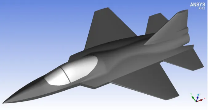
Figure 1.1: Conceptual design of the aircraft ... 2

Figure 1.2: Aircraft afterbody at NAR=1.8 ... 3

Figure 1.3: external flap angle 𝛽 ... 3

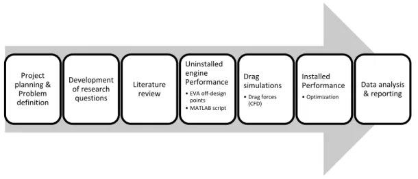
Figure 2.1: Flow scheme showing an overview of the study approach ... 5

Figure 3.1: Gas turbine station numbering ... 9

Figure 3.2: (a) overexpanded (b) Fully expanded (c) underexpanded ...14

Figure 3.3: Control volume V with surface element dS ... 17

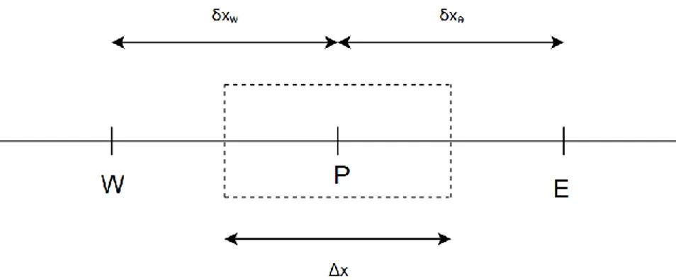
Figure 3.4: Illustration of a one-dimensional control volume ... 24

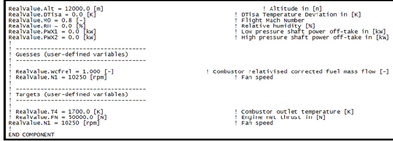
Figure 4.1: Screenshot of various off-design input parameters for EVA ... 27

Figure 4.2: Simulation scheme for engine performance for a Mach number ... 30

Figure 4.3: CFD simulation scheme at different Mach numbers ... 31

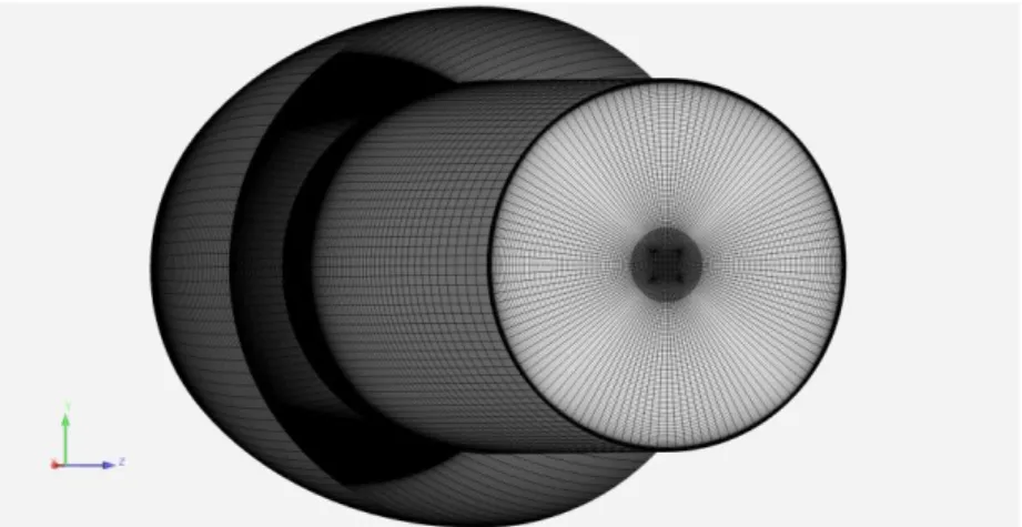
Figure 4.4: Aircraft and interface mesh ... 32

Figure 4.5: Nozzle geometry... 33

Figure 4.6: Nozzle mesh ... 33

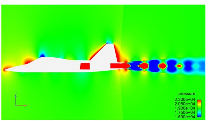
Figure 5.1: Pressure distribution over the aircraft body at Mach=0.8, NAR=1.55 & JPR=2 .. 40

Figure 5.2: Pressure distribution over the afterbody at Mach=0.8, NAR=1.55 & JPR=0.75 ...41

Figure 5.3: Pressure distribution over the afterbody at Mach=0.8, NAR=1.55 & JPR=2 ...41

Figure 5.4: Pressure distribution over the afterbody at Mach=0.8, NAR=2.05 & JPR=2 ... 42

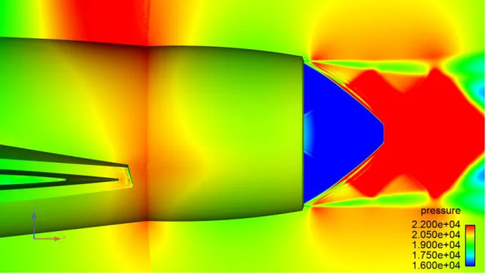
Figure 5.5: Pressure distribution over the aircraft body at Mach=1.4, NAR=1.55 & JPR=2 ... 42

Figure 5.6: Pressure distribution over the afterbody at Mach=1.4, NAR=1.55 & JPR=0.75 ... 43

Figure 5.9: Normal shock wave inside the nozzle at M=1.4, NAR=1.05 & JPR=0.75 ... 44

Figure 5.10: JPR as a function of NAR at Mach 0.6... 47

Figure 5.11: JPR as a function of NAR at Mach 0.8 ... 47

Figure 5.15: FG and FN at Mach 0.6 ... 49

Figure 5.20: Difference between installed and unistalled optimal area ratio at different Mach numbers ... 52

Figure 5.21: Thrust gain when using the optimal installed NAR ... 52

Figure 5.22: Thrust gain in percent when using the optimal installed NAR ... 53

Figure 5.23: Difference between installed and uninstalled optimal jet pressure ratio at different Mach numbers ... 53

(10)

TABLES

Table 4.1: Nozzle inlet conditions at different freestream Mach numbers ... 28

Table 4.2: Throat area at different Mach numbers ... 29

Table 4.3: Engine static inlet pressure ... 35

Table 4.4: Intake mass flow ratio for each Mach number ... 35

Table 4.5: Freestream velocity ... 37

Table 4.6: Freestream data ... 37

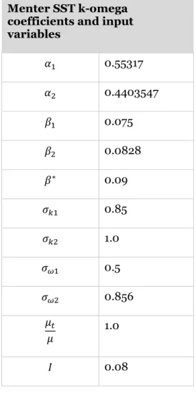
Table 4.7: Menter SST k-omega coefficients, viscosity ratio and turbulence intensity ... 38

Table 5.1: Normalized afterbody drag in Newton at Mach 0.6 from the CFD simulations ... 45

Table 5.6: Maximum and minimum normalized afterbody drag in Newton ... 46

NOMENCLATURE

Symbol Description Unit

ηAB Afterburner efficiency - ℎ Altitude 𝑚 𝑎𝑚𝑏 Ambient condition - 𝛼 Angle of attack - 𝐴 Area 𝑚2 𝐶𝐷 Cross-diffusion 𝑘𝑔 𝑚3_{∙ 𝑠}2 𝜌 Density 𝑘𝑔 𝑚3 𝐷 Diffusion coefficient 𝑚 2 𝑠 𝐶𝐷 Discharge coefficient − 𝐹𝐷 Drag N 𝐶𝑑 Drag coefficient - 𝜇 Dynamic viscosity 𝑘𝑔 𝑚 ∙ 𝑠 𝜇𝑡 Eddy viscosity 𝑘𝑔 𝑚 ∙ 𝑠

(11)

e Exit -

𝛽 External flap angle °

𝑭 Force vector 𝑁

∞ Freestream -

𝑊𝑓 Fuel mass flow 𝑘𝑔/𝑠

𝐹𝐴𝑅 Fuel to air ratio -

𝜑 General variable -

𝑆𝜑 General variable source _term -

∇ Gradient -

𝐹𝐺 Gross thrust 𝑁

𝑄̇ Heat W

𝑞̇ Heat transfer rate 𝐽

𝑠

𝑖 Internal energy 𝐽

𝑘𝑔

𝛿𝑖𝑗 Kronecker delta -

QLHV Lower heating value

𝑀𝐽 𝑘𝑔 𝑀 Mach number − 𝑚 Mass 𝑘𝑔 𝑚̇ Mass flow 𝑘𝑔/𝑠 𝛼1 Menter SST coefficient - 𝛼2 Menter SST coefficient - 𝛽1 Menter SST coefficient - 𝛽2 Menter SST coefficient - 𝜎𝑘1 Menter SST coefficient - 𝜎𝑘2 Menter SST coefficient - 𝜎𝜔1 Menter SST coefficient - 𝜎𝑘1 Menter SST coefficient - 𝜎𝑘2 Menter SST coefficient - 𝜎𝜔1 Menter SST coefficient - 𝜎𝜔2 Menter SST coefficient -

𝒈 Net body forces per unit _{of mass} 𝑁 𝑘𝑔

(12)

𝒏 Normal vector -

𝑒 Nozzle exit -

𝑃𝑟 Prandtl number -

𝑃𝑘 Production of turbulent _{kinetic energy}

𝐽 𝑠

𝑄̇𝑣𝑖𝑠𝑐𝑜𝑢𝑠 Rate of added heat

𝐽 𝑠

𝑊̇ Rate of work vector 𝑁𝑚

𝑠

𝑆𝑐 Schmidt number -

𝜆 Second viscosity 𝑘𝑔

𝑚 ∙ 𝑠 𝑆𝐹𝐶 _consumptionSpecific fuel 𝑘𝑔

𝑁 ∙ 𝑠 𝑐𝑝 Specific heat at constant _pressure

𝐽 𝑘𝑔 ∙ 𝐾 𝑐𝑣 Specific heat at constant _volume

𝐽 𝑘𝑔 ∙ 𝐾

𝛾 Specific heat ratio −

𝜔 Specific turbulent _{dissipation rate} 1 𝑠 𝑝 Static pressure 𝑃𝑎 𝑇 Static temperature 𝐾 𝜏 Stress tensor - 𝑆 Surface - 𝑘𝑡 Thermal conductivity 𝑊 𝑚 ∙ 𝐾 𝐶𝐹 Thrust coefficient − 𝑡 Time 𝑠 𝜌0 Total density 𝑘𝑔 𝑚3 𝐸 Total energy 𝐽 𝑝0 Total pressure 𝑃𝑎 𝑇0 Total temperature 𝐾 𝜖 Turbulence dissipation 𝐽 𝑘𝑔 ∙ 𝑠 𝐼 Turbulence intensity -

𝑘 Turbulent kinectic _energy 1 𝑠

(13)

𝑃𝑟𝑡 Turbulent Prandtel _number -

𝑅 Universal gas constant 𝐽

𝑘𝑔 ∙ 𝐾 𝑈 Velocity 𝑚 𝑠 𝐶𝑋 Velocity coefficient − 𝑼 Velocity vector 𝑚 𝑠 𝜇𝑡 𝜇 Viscosity ratio - 𝑭𝒗𝒊𝒔𝒄𝒐𝒖𝒔 Viscous Forces 𝑁 𝑉 Volume 𝑚3 𝑊̇𝑣𝑖𝑠𝑐𝑜𝑢𝑠 Work done 𝐽 𝑠

ABBREVIATIONS

Abbreviation Description

APA American Psychological Association – Referece system CD Convergent-Divergent (nozzle) – A combination of a

convergent and a divergent duct

CFD Computational Fluid Dynamics – Simulation method for simulating fluids mechanics

EVA EnVironment Assessment – A tool for novel propulsion system assessment

JPR Jet Pressure Ratio - The ratio between the jet exit-static pressure and the ambient pressure

MDH Mälardalens Högskola – Mälardalen university NAR Nozzle Area Ratio – The ratio between nozzle throat

area and nozzle exit area

SFC Specific Fuel Consumption – Ratio of the fuel mass flow and the thrust

RANS Reynolds Average Navier-Stokes – Fluid flow equations

(14)

1 INTRODUCTION

Modern fighter aircrafts use gas turbine engines that are incorporated into the fuselage that can propel the vehicle to even supersonic velocities. The nozzle is the instrument at the rear of the gas turbine with a certain geometry that allows the engine exhaust gases to expand and create useful thrust. The fundamental principle of how it operates is relatively simple but modelling its installed effect on afterbody drag becomes complex.

The rear part of the aircraft afterbody, is called nozzle external flaps can account for as much as 15% of the total drag over the body (Bergman, 1974). The afterbody is therefore certainly a significant component to consider when developing the aerodynamic design and configurations of the aircraft. A balance between maximizing the internal performance of the nozzle while minimizing the external drag of the afterbody must be obtained to ensure optimal performance. This proves challenging as improving on one may come at the sacrifice of the other (Carson Jr. & Lee Jr., 1981).

Additional challenge with aircraft design comes from the necessity to make them capable of operating in different flight conditions. The aircraft will be exposed to varying ambient conditions, as well as operating at different capacities during take-off and landing, subsonic cruise, supersonic cruise and maneuvering.

For the nozzle to be able to sufficiently accelerate the exhaust flow for any capacity or condition, the internal geometry is designed to be adjustable. The specific nozzle configuration is determined with the engine operating conditions at the nozzle inlet. These are the total states and mass flow. The variable nozzle geometry is therefore a tool to optimize the nozzle function, but it will also affect the external flow and drag over the afterbody.

Drag has adverse effect on operation as it leads to lower potential thrust and reduced efficiency. Fuel efficiency has significant implications on economy and design of the aircraft that could spiral into a feedback loop. Reduced fuel efficiency leads to increased fuel capacity necessity, which increases the weight of the aircraft and that results in even worse fuel efficiency. The aerodynamic design of the nozzle is therefore also an important element to consider when optimizing of the aircraft design for effects such as fuel efficiency.

1.1 Problem description and study object

Propulsion systems for aircraft vary depending on the certain operating conditions. Fighter aircrafts mainly use two jet engine types, which are turbojets and low-bypass turbofans, and these most often use a convergent-divergent (CD) nozzle. An afterburning low-bypass turbofan allows military aircrafts to combine two benefits: A high level of thrust with a small frontal area (Zukoski, 1978).

(15)

Engine manufactures supply the engine with the nozzle designed for maximum thrust. Although, the engine may not necessarily be optimized when installed in the aircraft. There will be drag effects over the afterbody, which may change the optimal point of operation for maximum thrust. The afterbody drag level is determined by the nozzle configuration, since it decides the afterbody geometry and the exhaust flow. At a specific operating condition, the nozzle has a fixed throat area. It makes the nozzle exit area the key factor in deciding the shape of the afterbody. This study develops a methodology for determining the optimal nozzle exit area for high-altitude cruising at maximum afterburner setting.

The studied object is a conceptual low bypass turbofan jet engine in the thrust class of the General Electric F414 engine (Gunston, 2004). It is a two-shaft low bypass turbofan engine with an afterburner for increased levels of thrust from the installed axisymmetric convergent-divergent nozzle. The engine is attached to a conceptual fighter aircraft geometry that was obtained from an open source CAD (GrabCad, 2018). The conceptual model is designed to resemble the fighter aircraft EADS Mako/HEAT.

Figure 1.1: Conceptual design of the aircraft

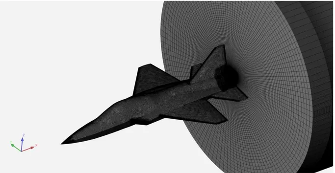
There is no single definition of what the aircraft afterbody should be defined as. Figure 1.2 shows the surface considered as the aircraft afterbody in this study. The end of the afterbody is called the external flap. In some studies, the external flaps are called aircraft boattail. The nozzle geometry varies at different settings since the external flap angle, or even known as boattail angle, is proportional to NAR.

(16)

Figure 1.2: Aircraft afterbody at NAR=1.8

Figure 1.3: external flap angle 𝛽

1.2 Aim

The aim of this report is to present a methodology for optimizing net thrust for the afterburning low-bypass turbofan engine in a conceptual aircraft model by finding the optimal axisymmetric nozzle configuration for different Mach numbers at an altitude of 12 km and 𝛼 = 0°. This will be accomplished by simulating the engine performance with EVA and MATLAB, and the drag forces over the afterbody with Computational Fluid Dynamics (CFD) using ICEM Mesh and M-Edge.

(17)

1.3 Research questions

How will different axisymmetric nozzle geometries affect afterbody drag at different freestream Mach numbers?

What effects will the nozzle exhaust flow have on afterbody drag?

What will be the differences between uninstalled and optimal installed engine performance?

1.4 Delimitations

The nozzle configuration will be optimized only for an angle of attack of 0°, an altitude of 12 km and with a specific fixed nozzle throat area for each specified freestream Mach number. This is because computational resources for a more extensive profile are not available. If they were, separate cases for different throat areas and varying altitudes could have been added to simulate a complete mission profile. However, the specific altitude should not have a great impact on results and the same conclusions would most likely be made.

The freestream Mach number range is chosen to be from 0.6 to 1.6. Any lower Mach numbers will have less effect on net thrust because the drag forces will be small. The upper Mach number limit of 1.6 is chosen, as the conceptual aircraft is not thought to exceed such speeds. Furthermore, the intake duct in the fictive aircraft is not designed to manage supersonic speeds. Therefore, the engine inlet static pressure was set to values that ensured that air mass flow passed through the intake duct.

The thrust will only be simulated at maximum afterburner power setting as to enhance the trends in the drag model. This is achieved by adding a conceptual afterburner that increases the total temperature in the nozzle inlet to 2000 K.

The nozzle geometry is determined with the length dimensions from (Carson Jr. & Lee Jr., 1981). The use of this theoretical design is to avoid studying the finess ratio as an additional parameter when a reasonable design concept could be used instead.

(18)

2 METHOD

The purpose of this section is to provide the reader with information about how this study was conducted. It will include descriptions of study design, literature review and ethical considerations. Firstly, the different approaches to address the problem are defined in the study design. Secondly, the methods used to search for appropriate literature will be explained in the literature review. Finally, the ethical principles considered in this study will be introduced.

2.1 Report structure

The following main chapters will be presented in this report: Introduction, method, literature study, methodology development, results, analysis, conclusions and future work. The MDH report template for energy technology was used and the APA reference guide was followed. According to Malcolm Chiswick (2004) experiencing difficulties to comprehend the content in scientific papers are most of the time related to the structure and presentation of the paper. To improve the comprehensibility throughout the report, instructions from Rolf Ejvegård’s book “Vetenskaplig metod” was used.

2.2 Study design

This study was a part of a master thesis at MDH during the period 2019-04-25 to 2019-08-23. It was a case study and a modelling task that was performed in collaboration with Saab in Linköping, in order to examine the significance of variable nozzle geometry when installed in an aircraft. The object to study in this master thesis was the afterbody of a conceptual fighter aircraft with an afterburning low-bypass turbofan engine. Access to Saab’s workspace, competence, equipment and data was made available for the purpose of the study.

Figure 2.1: Flow scheme showing an overview of the study approach

Project planning & Problem definition Development of research questions Literature review Uninstalled engine Performance • EVA off-design points • MATLAB script Drag simulations • Drag forces (CFD) Installed Performance • Optimization Data analysis & reporting

(19)

At first a proper problem definition was identified, and research questions were then formulated with the aim of framing interesting aspects of the problem. Literature was then reviewed to identify key elements and theories. Afterwards, an operating scheme for the CD nozzle was created. The operating scheme was based on isentropic relations for a CD nozzle and a gas turbine simulation model.

The tool used to simulate the gas turbine is called EVA and it simulated the conditions at the nozzle inlet. The total temperature into the nozzle was assumed be raised to 2000 K by an afterburner. These conditions were the backbone of constructing a mathematical model for the isentropic relations in MATLAB. The aim of the model was to find an appropriate nozzle throat area and uninstalled gross thrust at a specific operating condition.

A set of five operating conditions was later selected to frame a Mach number range of 0.6 to 1.6 at an altitude of 12 km. For each operating condition a fixed throat area was determined by employing the operating scheme. Different nozzle area ratios (NAR) were then examined to determine the uninstalled engine performance.

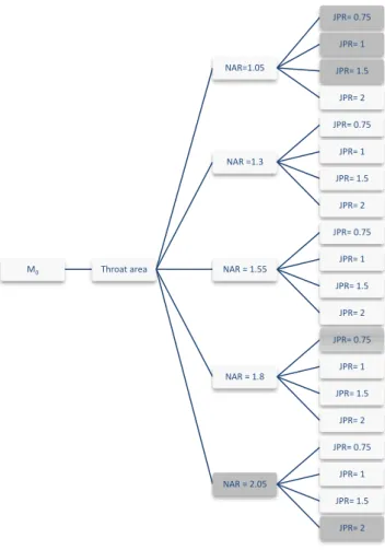
To investigate the installed engine performance, a drag model was created with CFD for a model of the aircraft and nozzle. At each Mach number, five NAR at; 1.05, 1.3, 1.55, 1.8 and 2.05, were used to examine the impact of variable nozzle exit area. Four different JPR were also examined for each area ratio. In total, 25 different nozzle configurations were modelled and a total of 100 simulations were executed.

The uninstalled engine performance and the drag forces were then combined to find the optimal installed engine performance at the different operating conditions. The aircraft body used in this study is fictive due to ethical consideration described in section 2.4. Further description of how each program was used will follow in the methodology section

.

2.3 Literature review

The literature study was constructed continuously during the study to ensure that important theories and equations were included. The aim of the literature study was to increase the theoretical knowledge of the subject. Using earlier studies empathises the credibility by supporting the arguments presented in discussions and conclusions.

Firstly, fundamental principles mainly from books were described to present broad information about gas turbines and fluid mechanics. This was made in order to create a foundation for the methodology and result sections where data and models were introduced. Finally, the literature review was dedicated to research articles and books that could be valuable when comparing and discussing the results. Additionally, brief research regarding the selected software was made. The choice of sources was handled with care to increase the credibility of the study and minimize the risk of including any uncertain information. The literature review was mainly based on books, websites and some scientific papers. The main databases used for finding the scientific articles were the “Scopus”, “Google Scholar” and “ScienceDirect”. National Aeronautics and Space Administration (NASA) website was used as compliment to the previous named references.

(20)

2.4 Ethical consideration

Ethics of research concerning honesty, objectivity, integrity, carefulness and, most significant for this study, confidentiality were considered. Generally, ethical principles are mostly discussed in combination with medical or social researches. However, most guidelines can be applied to any scientific study.

The data from this study is only gathered from conceptual cases and is not associated with any real application. Nevertheless, the results, discussions and conclusions from this study may be considered when creating a methodology to simulate and optimize nozzles.

(21)

3 LITERATURE STUDY

In this literature study, fundamental theories behind fluid mechanics, gas turbine engines and CFD are presented.

3.1 Jet engine

Jet engines increase the internal energy of the gases in order to accelerate them through a nozzle and thereby generate thrust. (Walsh & Fletcher, 2004; Saravanamuttoo et al, 2001;

Rolls Royce, 2005). Basically, air is inhaled into the engine, compressed, burned with fuel in

a combustion chamber and then expanded out through the turbine and nozzle (Shevell, 1989; Lefebvre & Ballal, 2010; Mattingly, 1996). Different gas turbine stations and station numbering used in this study is shown in Figure 3.1. The compressor consists of several stages to safely increase the pressure while not risking any backflow. It receives its energy from a turbine through the torque of a shaft between them. There are various types of jet engines: Turbofan, turbojet and ramjet are some examples.

Many fighter aircrafts currently use 2-shaft turbofan engines. The main difference compared to a simple jet engine is that these types of engines include two separate turbines and two separate compressors. A low-pressure turbine is connected to a separate shaft than the high-pressure turbine. The low-high-pressure turbine also drives a fan located at the front of the engine. In a turbofan, the intake air is divided into two flows where some of it continues into the core while the remaining air bypasses. Depending on the aircraft type, the bypass air is then either used for cooling or for thrust in a cold nozzle.

The cold nozzle is generally adopted in configurations with high-bypass ratios. In low-bypass application on the other hand, the air is most often used for cooling purposes or in a mixer to improve the propulsion efficiency (Walsh & Fletcher, 2004; Saravanamuttoo et al, 2001). Since fuel economy and noise reduction are not always priorities in military fighters, low-bypass turbofans are more favorable (Nicolas, 1997; NASA, 2015a). Afterburnung low-low-bypass turbofan engines produce a large amount of thrust from the highly accelerated jet stream, which allows for high flight velocities and compact engine designs (Austin Spang & Brown, 1999; Walsh & Fletcher, 2004). However, to secure an appropriate design, there are some constraints on how low the bypass must be. More airflow passing through the core requires more compressor work to reach efficient combustion (Priyant Mark & Selwyn, 2016).

Military fighter aircrafts mainly use CD nozzles. There are two types of CD nozzles: The first is mechanically locked without the ability to change NAR. The second is the variable nozzle type investigated in this study, which allows the throat area and the exit area to be adjusted individually and therefore change NAR.

(22)

Figure 3.1: Gas turbine station numbering

3.1.1 Convergent-divergent nozzle

The axisymmetric CD nozzle is the combination of a convergent duct followed by a divergent duct. The location at the transition is called the throat and this is where the cross-section area is the smallest throughout the nozzle. The relation between the area of the duct and the fluid velocity is derived from the continuity equation for isentropic inviscid adiabatic flow by Anderson Jr (2007) and is

𝑑(𝜌𝑈𝐴) = 0 (3.1)

The resulting area-velocity relation is 𝑑𝐴 𝐴 =(𝑀 2_{− 1}₎𝑑𝑈 𝑈 (3.2)

The decreasing cross-sectional area in the converging part of the nozzle increases the fluid velocity for subsonic flow. The fluid velocity also decreases with increasing area for subsonic flow. For supersonic flow the velocity instead increases with increasing axial area but the velocity decreases with decreasing axial area. If the Mach number is 𝑀 = 1, the right-hand side of equation (3.2) equal to zero. This corresponds to a mathematical extreme point, where there is no change in cross-sectional area. This is the throat of the nozzle.

The CD nozzle utilizes this principle to accelerate the flow to supersonic conditions by first accelerating the flow from subsonic velocity in the converging duct, to sonic velocity at the throat and then finally to supersonic velocity in the diverging duct (Anderson Jr, 2007). Just as the CD nozzle can be utilized to accelerate the flow from subsonic to supersonic velocity, the principle also allows for deceleration from supersonic to subsonic velocity with the same CD nozzle configuration (Anderson Jr, 2007).

Another important equation, which relates the Mach number with the ratio of the duct area A to the sonic throat area A*_{, is called the area-Mach number relation (Anderson Jr, 2007;} Munson et al., 2013). It is derived from the mass continuity for isentropic flow. This equation can be used to find the local Mach number at any location in the nozzle.

(𝐴 𝐴∗) 2 = 1 𝑀2[ 2 𝛾 + 1(1 + ( 𝛾 − 1 2 ) 𝑀 2_)] 𝛾+1 𝛾−1 _(3.3)

(23)

Two solutions can be obtained when using equation (3.3), one for the convergent region of the nozzle when M<1 and one for the divergent region of the nozzle when M>1. The relation between the Mach number, total conditions and static conditions for pressure, temperature and density can be calculated for an isentropic nozzle with the following equations for compressible flow (Anderson Jr, 2007).

𝑝 𝑝0 = (1 +𝛾 − 1 2 𝑀 2₎ − 𝛾 𝛾−1 (3.4) 𝑇 𝑇0 = (1 +𝛾 − 1 2 𝑀 2₎ −1 (3.5) 𝜌 𝜌0 = (1 +𝛾 − 1 2 𝑀 2₎ −_𝛾−11 (3.6)

3.1.2 Choked flow

There is a limit to the maximum mass flow of a fluid through a CD nozzle. This phenomenon starts at the throat at sonic conditions and continues in the divergent part of the nozzle when the fluid downstream can no longer communicate with the flow upstream. This is because the maximum speed at which the information of the fluid properties propagates through the flow is at the speed of sound. In the divergent part of the nozzle, the flow is supersonic, and the fluid moves faster than the speed of sound. This makes the fluid properties at the throat and upstream independent of the fluid properties downstream. Any further expansion of the flow in the divergent nozzle, that increases velocity and reduces pressure, will not increase the mass flow rate any further. When this happens, the flow is choked and the mass flow rate is determined by the throat area independent of how low the exit pressure is (Anderson Jr, 2007; Munson et al., 2013).

3.1.3 Compressible flow & shock waves

Flows within the supersonic region are subject to shock waves because of the compressibility of the fluid. Shock waves are rapid compression processes that change the properties of the flow across them (Anderson Jr, 2007). The two different types of show waves are: Normal shock waves and oblique shock waves. The velocity decreases across both types of shock waves, but it decreases down to subsonic velocity for normal shock waves. The total pressure also decreases across the shock waves. Because there is no work performed total enthalpy and total temperature is constant. The static conditions also change across the shock wave, increasing the static pressure, static temperature, density as well as the entropy.

Shockwaves occur in many locations over the aircraft body and become more prominent as Mach number increases. Notably, they occur both at the intake and also inside the nozzle. There will be normal shockwaves or oblique shockwaves either outside, in the entry or down

(24)

the intake duct depending on the design. This happens when the flow changed from supersonic velocity in the freestream to subsonic velocity in the intake. Inside the nozzle will either be a normal shock wave, depending on the conditions in the nozzle, or oblique shock waves in the divergent nozzle and jet plume.

3.1.4 Gross thrust

The thrust is the force that propels the aircraft forward and is created by the momentum and the pressure difference of the exit stream. If the exit pressure is larger than the ambient pressure, the surplus of pressure will create additional force over the exit area of the nozzle (Walsh & Fletcher, 2004; NASA, 2015c). The gross thrust can be calculated as

𝐹𝐺 = 𝑚̇9∗ 𝑈9 + (𝑝9− 𝑝𝑎𝑚𝑏) ∗ 𝐴9 (3.7)

3.1.5 Afterburner

To avoid installing large engines that increases the weight and the size of a fighter aircraft, an afterburner can be used as an alternative (Kundu, Price & Riordran, 2016; Walsh & Fletcher, 2004). An afterburner is a second combustions system that burns fuel with the remaining oxygen in the gas flow after the turbine (Zukoski, 1978). The exhaust gas temperature therefore increases significantly. This is often necessary to produce the massive amount of thrust that allows the fighter to accelerate to supersonic velocity (Saravanamuttoo et al, 2001).

Afterburners are installed before the exhaust nozzle and are connected to the turbine by a diffuser that decreases the fluid velocity of incoming air from the turbine (Saravanamuttoo et al, 2001; Zukoski, 1978). The application of an afterburner requires the nozzle throat to be adjustable as the throat area must be larger when the afterburner is in operation.

The increase in thrust is not obtained without trade-off (Saravanamuttoo et al, 2001; Zukoski, 1978). Since the pressure is much lower after the turbine, the combustion that takes place in the afterburner will not necessarily be as efficient as in the combustor. Evidently, using the afterburner will increase SFC drastically but the fighter will have much more capability when accelerating and manoeuvring (Saravanamuttoo et al, 2001; Zukoski, 1978).

3.2 Factors that impact performance

An aircraft engine is usually developed separately from the other components of the plane. The engine will therefore not necessarily be of optimal design when installed in the aircraft. The best engine configurations vary depending on the aircraft design.

Some examples of the losses in the installed engine are aerodynamic drag, viscous losses and pressure losses. These all have negative impact on performance. In other words, the engine

(25)

performance will be contingent on the operating conditions of the aircraft (Anderson Jr, 2012; Munson et al., 2011; Kundu et al., 2016).

The forgoing losses entail a decrease in generated thrust from the propulsion system and increased fuel consumption when the engine is installed in the aircraft. The total thrust losses due to installation effects can reach up to 15 % in fighter aircrafts. These losses will vary at different operating condition. For example: At take-off the thrust losses are between 7 -10 %, while cruising the corresponding value is typically 3-5 % (Kundu et al., 2016).

3.2.1 Aerodynamic drag

As an aircraft moves through the surrounding air it faces resistance by forces acting in the opposite direction of its flight path (Mattingly et al. 2000; Kundu et al., 2016). These forces are called drag forces and they are a penalty that arises for objects that is moving through any fluid. There are different types of drag forces. One is the form drag or also known as pressure drag that is created when the air is being pushed away from the aircraft (Anderson Jr., 2012). Another type is viscous drag that is associated with the friction forces over the aircraft surface (Anderson Jr., 2012; Mattingly et al. 2000).

Additional drag forces that must be considered are induced drag and wave drag (Anderson Jr., 2012). Induced drag is the result of the lifting force over the surface of the body, mainly the wings of the aircraft. Wave drag on the other hand is limited to transonic and supersonic flight. Accelerating to supersonic velocity causes shock waves around the aircraft that induces a large amount of drag.

Drag coefficient is an indicator of how easy the aircraft can move through air. It is defined as the relation between the drag force and the dynamic pressure and reference area

𝐶𝑑=

𝐹𝐷

(𝜌𝑈_{2 ) 𝐴}2

(3.8)

The drag coefficient over the aircraft is at its highest level at the point when the speed of sound limit is broken (Carson Jr. & Lee Jr., 1981). This is a result of the formation of shock waves over the plane at this velocity. The shock waves are a result of a rapid compression of the air by the aircraft that creates a massive change in air properties, such as pressure difference over the shock wave. This large variation in pressure causes an increase in drag. This is the reason aircrafts avoid cruising at transonic velocity. When the aircraft exceeds the speed of sound, however, most parts of the plane are travelling at supersonic speeds, which helps preventing boundary layer separation. (Carson Jr. & Lee Jr., 1981)

3.2.2 Afterbody drag

The drag over the external flaps of afterbody could account for about 15% of the total aircraft drag, depending on conditions and configuration (Bergman, 1974). It depends on several flow and geometrical factors and is difficult to estimate analytically. Two of the major effects that

(26)

are present is the jet plume effect and the entrainment effect (Carson & Lee, 1981). The jet plume effect reduces drag by pressurizing the end of the afterbody and the entrainment effect increases drag by increasing the external velocity over the afterbody, which reduces the pressure. These are mainly dependent on NAR and JPR.

3.2.2.1. Area ratio

The external flap angle changes with the variable nozzle exit area. Decreasing the external flap angle at the hinge simply increases the nozzle exit area. It is often determined as a relation between the exit area and the throat area.

𝑁𝐴𝑅 =𝐴9

𝐴8 (3.9)

Increasing the external flap angle increases the jet plume effect by changing the direction of the surface pressure more towards the upstream axial direction. Increasing the external flap angle also increases the entrainment effect. Compton and Runckel (1970) attribute this occasion to the greater external flow turn at smaller NAR. This turning of the flow increases the velocity of the fluid and therefore reduces the pressure over the afterbody. The net result from increasing the afterbody angle at subsonic flow tends to reduce drag up to an angle where the flow starts separating and the drag starts to increase as a result of the separation (Tran et al., 2019). Therefore, increasing the afterbody angle generally causes more favourable jet interference (Compton & Ruckel, 1970).

3.2.2.2. Pressure ratio

The jet effects have various influences on drag depending on freestream Mach number and nozzle pressure ratio, because they decide the structure of the flow on the aircraft afterbody. The nozzle pressure ratio is defined as the relation between the nozzle total inlet pressure and the static exit pressure

𝑁𝑃𝑅 =𝑝07

𝑝9 (3.10)

JPR can also be used to define the exhaust flow 𝐽𝑃𝑅 = 𝑝9

𝑝𝑎𝑚𝑏 (3.11)

It is important to notice the difference between NPR and JPR. NPR is the relation between the total pressure and the static exit pressure, while JPR is the ratio between the static exit pressure and the ambient pressure. Both NPR and the JPR can be used to describe the flow through the nozzle, and they are correlated with each other. A JPR less than 1 is an indication of overexpanded nozzle. While a JPR larger than 1 is a sign of underexpanded and if the JPR

(27)

Both underexpanded and overexpanded flows mean lower nozzle efficiency. In the case of underexpanded flow, the expansion will continue outside of the nozzle through expansion waves, which do not contribute to thrust. While if the flow is highly overexpanded, shock waves will occur in the nozzle and cause reduced efficiency.

(a) (b) (c)

Figure 3.2: (a) overexpanded (b) Fully expanded (c) underexpanded

Increasing JPR reduces the entrainment effect as the expanding jet diameter increases and the flow turning acceleration decreases. Increasing JPR also increases the jet plume effect that pressurizes the end of the afterbody. The high jet diameter helps to move the freestream acting upon the afterbody away from the centreline (Bergman, 1974; Compton & Runckel, 1970). Therefore, the flow will recompress more on the afterbody surface compared to design conditions.

At supersonic conditions, the exhaust flow creates a trailing shock wave over the afterbody (Carson & Lee, 1981; Donovan & Lawrence, 1957). The shock location over the afterbody is dependent on the JPR andincreasing it will force the shock wave upstream.

Increasing JPR therefore tends to have a favourable effect on the afterbody drag for both subsonic and supersonic conditions (Bergman 1974; Reubush, 1974; Harrington, 1969). Although, the positive effects of JPR are not as noticeable at small afterbody angels during either supersonic or subsonic conditions (Carson & Lee, 1981).

3.2.3 Nozzle performance

With the isentropic relations, shown in 3.1.1 and the thrust equation in section 3.1.4, the total states can be calculated for each station in the nozzle. It is however not realistic to assume isentropic conditions when estimating nozzles performance. When accounting for losses, the characteristics of the nozzle will differ. Some losses to mention are the losses caused by incomplete flow expansion and pressure losses due to viscous effects. In the coming sections some coefficients used to measure the real performance of nozzles will be described. These variables are highly dependent on the specific nozzle design.

3.2.3.1. Discharge coefficient C

D

When fluid flows through a pipe, duct or any other fixed surface, a layer around the walls of the surface will develop (Munson et al., 2011). This layer is called the boundary layer. Friction losses are created in the boundary layer because of the interaction between the surface and the fluid.

(28)

The principle of boundary layer is most important when explaining the discharge coefficient. Due to friction losses, the effective area, through where the fluid passes, differs from the real geometric area of a nozzle. It means that the viscous effects prevent the fluid from passing through the actual geometric area (Mattingly, Heiser & Pratt, 2000; Dixon & Hall, 2014). This flow behavior will cause a variation between the real mass flow and the theoretical mass flow and thereby create losses in thrust. The definition of the discharge coefficient can simply be expressed as the ratio of the real mass flow to the theoretical mass flow through the nozzle.

𝐶𝐷=

𝑚̇𝑟𝑒𝑎𝑙

𝑚̇𝑖𝑑𝑒𝑎𝑙

(3.12)

Since the area is the main influencing variable on the discharge coefficient, it can also be expressed as a function of the effective flow area and the actual geometric area.

𝐶𝐷=

𝐴𝑒𝑓𝑓

𝐴𝑔𝑒𝑜

(3.13)

3.2.3.2. Velocity coefficient C

X

As mentioned earlier, the velocity of the flow increases both in the convergent and the divergent region of the nozzle at choked conditions. For non-ideal calculations, the velocity coefficient is used as an indicator of the degree of velocity losses caused by the viscous effects in the nozzle. These losses occur due to shear stress, which is a force that hinders the movement of a flow. When the fluid is in contact with a pipe or a surface it slows down due to shear stress from the roughness of the pipe wall (Anderson Jr, 2012; Munson et al., 2011). The pressure will then drop and therefore reduce the exit velocity. The fundamental principle behind this phenomenon is the viscosity of fluids and in some cases the density.

Higher viscosity means larger friction force, which restricts the fluid from flowing (Munson et al., 2011). The temperature has a major impact on the viscosity of fluids and most gases will flow more easily at lower temperatures, while liquids tends to have higher viscosity at low temperatures.

The velocity coefficient can be defined as the ratio between the actual velocity and the ideal velocity of the exhaust gas at the nozzle exit (Mattingly et al. 2000). Since the thrust is dependent to the jet velocity, this parameter, as well as the discharge coefficient, will have an impact on the nozzle performance.

𝐶𝑋 =

𝑈9

𝑈9𝑖𝑑𝑒𝑎𝑙

(3.14)

The denominator is the ideal velocity that can be achieved in the case if losses are neglected and the nominator is the actual velocity of the exhaust gas. The normal range for the velocity coefficient is between 0.95<Cx<0.98 (Sforza, 2012).

(29)

3.2.3.3. Thrust coefficient C

F

Supersonic flight requires high-pressure ratio over the nozzle, which makes it crucial to use a convergent-divergent nozzle to reduce the thrust losses (Mattingly et al. 2000; Walsh & Fletcher, 2004). The ratio between the real thrust and the ideal thrust is described by the thrust coefficient. It is another variable that is used to evaluate the performance of nozzles. (Mattingly et al. 2000; Walsh & Fletcher, 2004).

𝐶𝐹=

𝐹𝐺𝑟𝑒𝑎𝑙

𝐹𝐺𝑖𝑑𝑒𝑎𝑙

(3.15)

The term in the denominator is the ideal thrust produced when the flow expands completely to equal the ambient pressure, and where no viscous losses and mass flow losses occur (Mattingly et al. 2000; Walsh & Fletcher, 2004).

3.3 Computational fluid dynamics

CFD is the method of using numerical algorithms to compute and determine the behavior of fluids. CFD simulations are created from two main elements: Pre-processing and solving. Pre-processing is the first step where the computational domain is first determined and where the geometry of the region is then created and subdivided into smaller domains or cells in a mesh (Versteeg & Malalasekera, 2007). The physical properties of the domain and the settings of the mesh are then also determined.

The solver then uses numerical solution technique to approximate the unknown flow variables and then solve the algebraic equations as partial differential equations (Versteeg & Malalasekera, 2007). The numerical solution then presents results that that can be interpreted in different manners. This is a third element beyond CFD called post-processing. It is a method to visualize the solution and to present clear illustrations of how the flow develops or how the heat changes through the fluid.

The theory behind fundamental fluid mechanics for the Eulerian description will be presented in the following section. The conservative governing equations for transient three-dimensional fluid flow and heat transfer of compressible Newtonian fluids are derived for mass transfer, momentum and energy. A turbulence model and the solution method of finite volume will then lastly be described.

3.3.1 Continuum mechanics

The Eulerian description depicts fluid motion at points in space and time within a fixed control volume instead of following an individual particle through the fluid (Rao, 2017). The control volume V with a surface S consists of infinitesimally small volume elements dV and infinitesimally small area elements dS. The physics of such systems can be modelled by continuum mechanics that describes the system as a continuous mass instead of a discrete atomic structure of individual particles (Rao, 2017). The substance that is modelled is

(30)

therefore assumed to completely fill the volume it occupies, but where dV is still large enough to be considered a continuous medium.

There can be closed systems that are defined as having no transfer of properties outside of the system boundaries such as matter, momentum or energy. The closed nature of such systems allows for three conservation principles to be applied as the conservation of mass, momentum and energy (Anderson Jr, 2007). These principles all follow the first law of thermodynamics which states that the total energy in a closed system must remain constant. This allows for the derivation of equations that determine the fundamental physical principles of a fluid moving through a fixed control volume. These final equations are called the governing equations and are known as Navier-Stokes equations of continuity, momentum and energy. They will be derived as done by Anderson Jr (2007).

3.3.2 Continuity equation

Mass can not be created nor destroyed. The continuity equation is derived from the conservation of mass and it follows the physical principle that mass must remain constant in a closed system. Therefore, it follows that the net mass flow out of a control volume through its surface must equal the rate of change of the mass inside the control volume.

Let V be an arbitrary control volume with surface S. It has a surface element dS with the normal vector n that is oriented to point out of the control volume.

Figure 3.3: Control volume V with surface element dS

The vector surface area element is then dS=ndS. Let 𝑼 = [ 𝑢 𝑣 𝑤

] be the local velocity vector and 𝜌 the density, then the mass flow across the area element dS is

𝜌𝑼𝒅𝑺 = 𝜌𝑼 ∙ 𝒅𝑺 (3.16)

The net flow of mass out of V through dS is then ∯ 𝜌𝑼 ∙ 𝒅𝑺_𝑆 . Applying the divergence theorem then gives

(31)

∯(𝜌𝑼 ∙ 𝒅𝑺)

𝑆

= ∰ ∇ ∙ (𝜌𝑼) 𝑑𝑉

𝑉

(3.17)

The mass contained within the volume element dV is 𝜌𝑑𝑉 and the total mass inside V is therefore ∰ 𝜌𝑑𝑉_𝑉 . The rate of decrease of the mass inside V is

− 𝜕 𝜕𝑡∰ 𝜌 𝑑𝑉 𝑉 = − ∰𝜕𝜌 𝜕𝑡 𝑑𝑉 𝑉 (3.18)

The net mass flow out of the control volume through the surface and the rate of change of the mass inside the control volume is

∰ ∇ ∙ (𝜌𝑼)𝑑𝑉 𝑉 + ∰𝜕𝜌 𝜕𝑡 𝑑𝑉 𝑉 = 0 (3.19)

This can be simplified as

∰ [𝜕𝜌

𝜕𝑡+ ∇ ∙ (𝜌𝑼)] 𝑑𝑉

𝑉

= 0 (3.20)

Since V is an arbitrarily chosen volume then the only way the integral can be equal to zero is when the expression in the brackets are equal to zero. Therefore, the equation can be reduced to

𝜕𝜌

𝜕𝑡+ ∇ ∙ (𝜌𝑼) = 0 (3.21)

This is the Navier-Stokes continuity equation as a partial differential equation.

3.3.3 Momentum equation

Newton’s second law of motion states that the sum of all forces acting on a body is equal to its time rate of change of momentum. It can be written in the general form as

𝑭 = 𝑑

𝑑𝑡(𝑚𝑼) (3.22)

Consider the right-hand side as the rate of change of momentum over time of a fluid as it flows through V. This rate of change is the sum of two terms. The first is the net change of momentum out of the control volume V over the surface S. The second is the rate of change of momentum over time due to unsteady fluctuations of flow properties inside V. These two terms are derived from the continuity equation, which represents the mass flow, then by scalar multiplication with the velocity vector U, the momentum is obtained.

(32)

𝑑 𝑑𝑡(𝑚𝑼) = ∯(𝜌𝑼 ∙ 𝒅𝑺)𝑼 𝑆 + 𝜕 𝜕𝑡∰ 𝜌 𝑼𝑑𝑉 𝑉 (3.23)

The forces acting on the fluid comes from two sources. The first source is the body forces acting inside V such as gravitational, electromagnetic or inertial forces for example. The second source is the surface forces acting on S such as pressure forces and shear stresses. Let

g represent the net body forces per unit of mass that is exerted on the volume element dV.

The total body forces exerted within V are then ∰ 𝜌𝒈𝑑𝑉_𝑉 . The total pressure over S is − ∯ 𝑝𝒅𝑺_𝑆 . The total force that is experienced by a fluid that is flowing through V is the sum of the body forces, the pressure forces and the viscous forces.

𝑭 = ∰ 𝜌𝒈𝑑𝑉

𝑉

− ∯ 𝑝𝒅𝑺

𝑆

+ 𝑭𝑉𝑖𝑠𝑐𝑜𝑢𝑠 (3.24)

The integral form of the momentum equations is then obtained by combining the previous equations as ∯(𝜌𝑼 ∙ 𝒅𝑺)𝑼 𝑆 + 𝜕 𝜕𝑡∰ 𝜌 𝑼𝑑𝑉 𝑉 = ∰ 𝜌𝒈𝑑𝑉 𝑉 − ∯ 𝑝𝒅𝑺 𝑆 + 𝑭𝑉𝑖𝑠𝑐𝑜𝑢𝑠 (3.25)

By applying the divergence theorem, and separating the surface pressure into static pressure p and the stress tensor 𝝉, the equation can be rewritten as

∰ [𝜕 𝜕𝑡(𝜌𝑼) + ∇ ∙ (𝜌𝑼 𝑻_{𝑼) + ∇ ∙ p − ∇ ∙ 𝝉 − 𝜌𝒈 − 𝑭} 𝑉𝑖𝑠𝑐𝑜𝑢𝑠] 𝑑𝑉 𝑉 = 0 (3.26)

The stress tensor 𝝉 models the viscous stresses over the surface of a body as 𝝉 = [

𝜏𝑥𝑥 𝜏𝑥𝑦 𝜏𝑥𝑧

𝜏𝑦𝑥 𝜏𝑦𝑦 𝜏𝑦𝑧

𝜏𝑧𝑥 𝜏𝑧𝑦 𝜏𝑧𝑧

] (3.27)

The viscous stresses can be understood by first defining the shear stress at the surface parallel to a body as

𝜏𝑦 = 𝜇

𝜕𝑢

𝜕𝑦 (3.28)

The viscous stresses over the surface is then defined as 𝜏𝑥𝑦 = 𝜏𝑦𝑥= 𝜇 ( 𝜕𝑢 𝜕𝑦+ 𝜕𝑣 𝜕𝑥) (3.29) 𝜏 = 𝜏 = 𝜇 (𝜕𝑢+𝜕𝑤) _(3.30)

(33)

𝜏𝑦𝑧= 𝜏𝑧𝑦= 𝜇 (

𝜕𝑣 𝜕𝑧+

𝜕𝑤

𝜕𝑦) (3.31)

The viscous stresses normal to the surface of the body is then defined as 𝜏𝑥𝑥 = 𝜆(𝛻 ∙ 𝑼) + 2𝜇 ( 𝜕𝑢 𝜕𝑥) (3.32) 𝜏𝑦𝑦 = 𝜆(∇ ∙ 𝑼) + 2𝜇 ( 𝜕𝑣 𝜕𝑦) (3.33) 𝜏𝑦𝑦 = 𝜆(∇ ∙ 𝑼) + 2𝜇 ( 𝜕𝑤 𝜕𝑧) (3.34)

Where 𝜆 is know as the second viscosity and often substituted as −2

3𝜇. For the same

reasoning as for the continuity equation, equation (3.26) must be identically zero at all points in the flow and can therefore be written as

𝜕

𝜕𝑡(𝜌𝑼) + ∇ ∙ (𝜌𝑼

𝑻_{𝑼) = −∇ ∙ p + ∇ ∙ 𝝉 + 𝜌𝒈 + 𝑭}

𝑉𝑖𝑠𝑐𝑜𝑢𝑠 (3.35)

This is the instantaneous Navier-Stokes momentum equation.

3.3.4 Energy equation

The governing equation for energy is derived from the first law of thermodynamics, which states that energy can neither be created nor destroyed. Applying this law to a control volume, the rate of change of energy for the fluid flowing through V must be equal to the rate of heat added and work done to V. The total rate of volumetric heating can be expressed as ∰ 𝜌𝑞̇𝑑𝑉_𝑉 + 𝑄̇𝑣𝑖𝑠𝑐𝑜𝑢𝑠, and the rate of work on a moving body is

𝑾̇ = 𝑭 ∙ 𝑼 (3.36)

Considering the right-hand side of the integral form of the momentum equation (3.25), the total rate of work done on the fluid inside V is expressed by scalar multiplication of the velocity vector U for the surface forces, the body forces and the viscous forces.

𝑼 [∰ 𝜌𝒈𝑑𝑉 𝑉 − ∯ 𝑝𝒅𝑺 𝑆 + 𝑭𝑉𝑖𝑠𝑐𝑜𝑢𝑠] = − ∯ 𝑝𝑼 ∙ 𝒅𝑺 𝑆 + ∰ 𝜌(𝒈 ∙ 𝑼)𝑑𝑉 𝑉 + 𝑊̇𝑣𝑖𝑠𝑐𝑜𝑢𝑠 (3.37)

(34)

The random motion of the atoms and molecules in the fluid is denoted as the internal energy per unit of mass 𝑖. A moving fluid inside is V with the velocity vector V has a kinetic energy. The sum of the internal and kinetic energies is called the total energy and the net flow of this across surface S can be expressed as ∯ (𝜌𝑼 ∙ 𝒅𝑺)_𝑆 (𝑖 +𝑈2

2). The total energy E can be expressed

as (𝑖 +𝑈2

2) and the change of the total energy inside V over time due to transient variations of

the variables can be expressed as 𝜕

𝜕𝑡∰ 𝜌 𝐸𝑑𝑉𝑉 . The integral form of the energy equation can

be expressed as an equality between rate of change of the energy inside V over time and the net rate of flow of energy across S with the rate of total heat addition and the rate of total work done on the fluid.

∯(𝜌𝑼 ∙ 𝒅𝑺) 𝑆 𝐸 + 𝜕 𝜕𝑡∰ 𝜌 𝐸𝑑𝑉 𝑉 = ∰ 𝜌𝑞̇𝑑𝑉 𝑉 + 𝑄̇𝑣𝑖𝑠𝑐𝑜𝑢𝑠− ∯ 𝑝𝑼 ∙ 𝒅𝑺 𝑆 + ∰ 𝜌(𝒈 ∙ 𝑼)𝑑𝑉 𝑉 + 𝑊̇𝑣𝑖𝑠𝑐𝑜𝑢𝑠 (3.38)

By applying the divergence theorem and setting the volume integral to be equal to zero for all points, the partial differential equation for the energy equation can be simplified to

𝜕

𝜕𝑡𝜌𝐸 + ∇ ∙ (𝜌𝐸𝑼) = 𝜌𝑞̇ − ∇ ∙ (𝑝𝑼) + 𝜌(𝒈 ∙ 𝑼) + 𝑄′̇𝑣𝑖𝑠𝑐𝑜𝑢𝑠+ 𝑊′̇𝑣𝑖𝑠𝑐𝑜𝑢𝑠 (3.39) The heat flux can be expressed in terms of volumetric heating such as absorption or emission of radiation. The heat transfer across the surface can be expressed as thermal conduction as

𝑄′̇𝑣𝑖𝑠𝑐𝑜𝑢𝑠= 𝑘𝑡𝑇(∇ ∙ ∇𝑇) _(3.40)

The rate of work done on the fluid due to viscous stresses can be expressed as 𝑊′̇𝑣𝑖𝑠𝑐𝑜𝑢𝑠= (∇ ∙ 𝝉) ∙ 𝑼𝑇

(3.41)

The viscous stresses can be expressed with the dynamic viscosity and the second viscosity as done for the momentum equation. The general energy equation for unsteady, compressible, three-dimensional, viscous flow can then be expressed as

𝜕

𝜕𝑡𝜌𝐸 + ∇ ∙ (𝜌𝐸𝑼) = 𝜌𝑞̇ − ∇ ∙ (𝑝𝑼) + 𝜌(𝒈 ∙ 𝑼) + 𝑘𝑡𝑇(∇ ∙ ∇

𝑇_{) + (∇ ∙ 𝝉) ∙ 𝑼}𝑇

(3.42)

(35)

3.3.5 Turbulence modelling

A unit of measurement of the relative importance of inertia forces and viscous forces for fluid flow is represented by the Reynolds number (Versteeg & Malalasekera, 2007). When the fluid is flowing in an orderly fashion in adjacent layers the flow is called laminar, which occurs for lower Reynolds numbers (Versteeg & Malalasekera, 2007). When the Reynolds numbers instead enters the regime of larger values, the flow begins to behave in a random and chaotic way (Versteeg & Malalasekera, 2007). This flow is called turbulent and its unsteady motion makes the velocity and the other flow properties adapt this complicated behaviour. Due to the nature of turbulent flow, it is incredibly difficult to model and predict.

In practice, it is often enough to calculate the time-average properties of a flow that follows the same expression. The flow property for the velocity vector is denoted as 𝑼_𝑖 and it is the sum of the steady mean component 𝑼̅_𝑖_{and the fluctuating component 𝑼′}_𝑖_.

𝑼𝑖= 𝑼̅𝑖+ 𝑼′𝑖 (3.43)

The Navier-Stokes equations for continuity and momentum can be written as time-average for turbulent flow. The Reynolds average Navier-Stokes equations (RANS) for continuity and momentum can be written in Cartesian tensor form as

𝜕𝜌

𝜕𝑡+ ∇𝑖∙(𝜌𝑢𝑖) = 0 (3.44)

𝜕

𝜕𝑡(𝜌𝑼𝑖) + ∇𝑗∙ (𝜌𝑼𝑖𝑼𝑗) = −∇𝑖∙ 𝑝 + ∇𝑗∙ 𝝉𝒊𝒋+ ∇𝑗∙ (−𝜌𝑼′̅̅̅̅̅̅̅̅) 𝑖𝑼′𝑗 (3.45) The −𝜌𝑼′̅̅̅̅̅̅̅̅̅𝑖𝑼′𝑗 term is of the Reynold stresses in the RANS equations. These are modelled with

the Boussinesq assumption (FOI, 2007). −𝜌𝑼̅̅̅̅̅̅̅̅′𝑖𝑼′𝑗= 𝜇𝑡[ 𝜕𝑼𝑖 𝜕𝑥𝑗+ 𝜕𝑼𝑗 𝜕𝑥𝑖− 2 3(∇𝐔)𝛿𝑖𝑗]− 2 3𝜌𝑘𝛿𝑖𝑗 (3.46)

3.3.6 Menter SST 𝒌 − 𝝎 turbulence model

A common turbulence model is the Menter SST k − ω model. M-Edge (Eliasson, 2002) (former CFD solver Edge) uses an alternative version that is blending the standard k − ε in the outer part of the boundary layer with the Wilcox k − ω in the near part of the boundary layer (FOI, 2007). This transforms the k − ε model into the k − ω with an added cross-diffusion term from Kok (2000) and with different coefficients. The turbulent kinetic energy is defined in (FOI, 2007) as

𝑘 =1 2𝑼̅̅̅̅̅̅ 𝑖𝑼𝑖

OPTIMIZATION OF NOZZLE SETTINGS FOR A FIGHTER AIRCRAFT