Real-time control in industrial IoT

V¨

aster˚

as, Sweden

Thesis for the Degree of Master of Science in Intelligent Embedded

System 30.0 credits

REAL-TIME CONTROL IN

INDUSTRIAL IOT

Alma Didic

adc13001@student.mdh.se

Pavlos Nikolaidis

pns13002@student.mdh.se

Examiner: Moris Behnam

M¨

alardalen University, V¨

aster˚

as, Sweden

Supervisor: Saad Mubeen

M¨

alardalen University, V¨

aster˚

as, Sweden

Company supervisor: Kristian Sandstr¨

om

ABB Corporate Research, V¨

aster˚

as, Sweden

Company supervisor: Hongyu Pei Breivold,

ABB Corporate Research, V¨

aster˚

as, Sweden

Acknowledgements

We would like to thank our supervisor from MDH Dr. Saad Mubeen, our supervisors from ABB Professor Kristian Sandstr¨om and Dr. Hongyu Pei Breivold for the collaboration and guidance during the thesis. We would also like to thank our examiner Dr. Moris Behnam for his precious help and advice.

Abstract

Great advances in cloud computing have drawn the interest of industry. Cloud infrastructures are used, mainly, for monitoring the shop floor. In recent years cloud technologies combined with IoT technologies have initiated the effort to close loops between industrial applications and cloud infras-tructures. This thesis examines the effect of including remote servers, both local and centralized, in the closed control loop. Specifically, we investigate how delays and jitter affect the closed control loop. A prototype is developed to include servers on a control loop and inject delays and jitter in the network. Furthermore, delay mitigation mechanisms are proposed and, using the prototype, a number of experiments are performed to evaluate them. The mitigation mechanisms focus mainly on delays and jitter that are larger than the period of closed control loop. The proposed mechanisms improve the closed control loop response but still fall short compared to the performance of the close control loop when it executes locally, without any servers included. We also, show that local servers can be included in the closed control loop without significant degradation in the performance of the system.

Table of Contents

2.3.3 Fog and similar technologies . . . 4

2.3.4 Fog architecture . . . 5

2.3.5 Another definition of Fog computing . . . 6

2.4 Offloading . . . 6

2.4.1 Definition . . . 6

2.4.2 Computational offloading approaches . . . 7

2.5 Industrial automation systems . . . 8

2.5.1 Automation . . . 8

2.5.2 Cloud-based automation . . . 10

2.5.3 Fog in industrial applications . . . 10

2.5.4 Smart factory . . . 11 3 Research method 12 4 System development 14 4.1 Architecture overview . . . 14 4.2 Design . . . 14 4.2.1 System design . . . 14

4.2.2 Delay mitigation mechanisms . . . 17

4.3 End device set-up . . . 19

5 Experimental evaluation 20 5.1 Experimental set-up . . . 20 5.2 Local Response . . . 20 5.2.1 Constant delays . . . 21 5.2.2 Jitter . . . 22 5.2.3 Discussion . . . 24 5.3 Delay mitigation . . . 26 5.3.1 Prediction methods . . . 26 5.3.2 Adaptive PI controller . . . 31 6 Related work 35 6.1 Cloud and Fog architectures . . . 35

6.2 Offloading . . . 35 6.3 Cloud-based automation . . . 35 6.4 Discussion . . . 36 7 Conclusion 37 8 Future work 38 9 References 39

1

Introduction

Technology has gone through a big boost in the recent years. The arrival of cloud computing has made sharing and accessing data an everyday occurrence. It has made working with big streams of data easy and manageable. It supports the storage of such data with flexibility.

The development of Internet of things (IoT) [1] has brought connectivity among the most diverse devices and has introduced a new kind of data flow. The future of IoT will bring even more connectivity and interaction among the simplest and most common devices (e.g., light bulbs and toasters). The IoT is therefore bringing more and more devices into the connected world, while cloud computing is able to support more and more users and their increasing amount of data. It is clear that both of these technologies are on the rise and are here to stay. It is only natural that these two technologies start coming together at some point.

The automation Industry is an area that uses both of these technologies. Having the end devices connected and networking together enables them to send and receive the information from each other. This means that practically the devices can demand the information when they need it instead of waiting for a scheduled response. It simplifies task scheduling as well as the scalability of the system. Having a cloud supervise all the data flow is beneficial for fault detecting and maintenance monitoring. Cloud computing can also be used as a way to backup a great amount of data. Furthermore, clouds can be used on a higher level between multiple plants to improve efficiency and collaboration between them at different sites.

1.1

Problem statement

Cloud computing and IoT are typically used at different levels. IoT, which is used at lower levels, deals mostly with the end devices, their connections and the protocols they use. Cloud computing is used at higher levels with the end users and deals with handling and storage of data. In other words, IoT works with low latency and, in the industrial automation, real-time environment. On the other hand, the cloud is connected to the system through a Wide Area Network (WAN) and therefore, it has unpredictable latencies. Thus, the following question comes to mind:“Is it possible to construct a stable and reliable control system while using cloud computing as a part of it?” If the cloud is brought closer to the devices, making a more secure and stable connection, there is no doubt that the automation industry will benefit from it. It would enable a centralized control while minimizing costs. But moving parts of the control system is not simple since it can affect the stability, robustness and reliability of the system.

1.2

Thesis goal

The goal of this thesis is to investigate ways of using the cloud in a closed loop control system and the impacts it will have on the system itself. The thesis includes building a prototype to asses the effects of having the cloud in the control system and evaluating the results.

1.3

Thesis outline

The rest of the thesis is organized as follows: Section 2 explains the terms and relevant technologies which are used throughout the document. Section 3 presents the research method that is used in this thesis. Section 4 explains the prototype system and its architecture. Section 5 presents the experimental evaluation. Section 6 summarizes the related work done in this and related fields. Finally, Section 7 concludes the thesis and Section 8 presents the recommendations for the future work.

2

Background

2.1

Internet of Things

The internet of things (IoT) is a term that first showed up in 1999 and in the recent years quickly gained wide popularity. It depicts an idea of various devices, such as sensors and embedded devices - the things, being connected to each other through the internet and using it as a means of sharing data and information. The things might have some level of intelligence that enables them to be aware of the surroundings and act accordingly. This simple idea offers a lot of potential to a wide range of fields and applications (health monitoring, home automation, ambient intelligence, augmented reality applications, smart cars, smart cities, ...) so it is not a big surprise it has gained such a huge following. But because it covers such a wide range it makes it hard to narrow down or generalize the fundamental characteristics of the IoT concept. There is no set definition of the term and different authors emphasize different aspects of it. Some focus on the networking or the connectivity of the devices and the way this connectivity is achieved, others focus on the fact that the things are embedded devices with limited resources and power saving features. One of the more general definitions, taken from [2] is:

“The Internet of Things (IoT) is the interconnection of uniquely identifiable embed-ded computing devices within the existing Internet infrastructure. Typically, IoT is expected to offer advanced connectivity of devices, systems, and services that goes be-yond machine-to-machine communications (M2M) and covers a variety of protocols, domains, and applications.”

As the idea of many connected devices grew into separate fields, many new concepts started forming. This, however, created a big pool of terms that are sometimes used interchangeably such as Web of Things (WoT), Internet of Everything (IoE), Embedded Web, Future Internet of Things (FIoT). Some even equalize it with more specific terms such as Machine-to-Machine (M2M) or even Industrie 4.0. It is important to note that the IoT is the most general term and although it might be related to a large part of what all of these terms specify. However, all these other terms are created for some specific sub-area which it focuses on and shouldn’t be confused with IoT.

Since the IoT networks simple embedded devices, limited by their CPU capabilities, power sources and memory, it naturally found its way into many applications. Some fields, like automation and ambient intelligence, were not part of the original idea, especially since they don’t require an internet connection. However, the potential of a great number of networked embedded systems is large, whether to expand the limited functionalities of the devices or to better utilize the massive amount of data they create. This also led to the development of cyber-physical systems (CPS), automated systems that connect the operations of the physical reality to communication and computing infrastructures [3]. While traditional embedded systems focus more on the computing abilities, the CPS focus more on the connection between the physical and computational elements. Research studies from Gartner [4] predict that there will be around 26 billion devices connected through the IoT by 2020. Such a number will have a huge impact on many things, not only on technology development [5]. For example, the IoT will require the use of IPv6 since using IPv4 would not be enough to support this amount of devices. Another problem that is considered in some papers is the amount of electronic waste that will build up, as well as the availability of materials that are used for making electronics (since very little is recyclable from old circuits). Another challenge is adapting to the impact of the changes that will come with the inevitable changes in existing business models. Job structures will change as many labour jobs become replaceable by machines and new maintenance jobs are formed instead. But the biggest challenge with IoT is privacy and security. The existing internet infrastructure is far from perfect when it comes to keeping the data safe. Having a big number of devices harvesting sensitive data from public places raises a lot of privacy and security concerns which current legislations cannot handle (for example data ownership). This implies that there is a need for some form of governance. That is, a governing body is needed to create and enforce policies that deal with such problems [5].

There is a great need for standardization as well, to ensure interoperability not only for the existing IoT frameworks but also for the future ones. There have been some efforts to introduce

an architectural reference model, like the IoT-A1_{project. In any case all agree that this area will}

expand rapidly in the next few years and that it will have both social and economical impacts on the industry, the workers and generally the countries that adopt it.

2.2

Cloud computing

Cloud computing was first introduced around 2000 and rapidly became popular. It was fully developed through the first decade of the twenty first century and reached the peak of inflated ex-pectations by the end of the decade. Grid and cluster computing architectures are the predecessors of the cloud architecture. Cloud architecture is based on aggregation of hardware components that are accessed and used as a unified entity. The details of the aggregation are hidden to the user and thus the complexity of scaling up is negligible. Scalability along with pay-as-you-go charging policy applied by cloud providers introduced a new operational and business model. Utilizing cloud computing, enterprises can take advantage of powerful infrastructures and, in parallel, minimize the operational, acquisition and maintenance costs by exploiting the pay-as-you-go policy. Con-sequently cloud computing drew the attention of industries that were interested in computational resources and big data analysis.

The great interest of companies in cloud computing increased the number of cloud providers, resulting with more than 200 cloud providers around the world in 2014, providing a big variety of services2. Cloud services are divided in three main categories: Infrastructure as a Service (IaaS), Platform as a Service (PaaS) and Software as a Service (SaaS). IaaS provides computational power and storage as a service (CPU, HDD etc.). Resources can be scaled up or down on demand in order to adapt the fluctuating demands. PaaS targets software developers and is indented to help them during the development process. Developers can utilize the service to develop, test and maintain software in a collaborative environment. SaaS offers commercial software applications hosted in remote data centers that can be accessed from everywhere. Amazon Web Services and Rackspace3

are examples of IaaS services, Google App Engines and Microsoft Azure Services4 _{are examples of}

PaaS services and finally SaaS example applications are Google Mail and Google Docs.

Cloud computing comes with significant advantages for industries but not for all kinds of applications. Firstly, latency-sensitive applications cannot be hosted in cloud infrastructure due to unpredictable and high latencies introduced by Wide Area Networks (WAN). Secondly, data privacy is one of the major drawbacks of cloud computing for industries. In order to reach the cloud infrastructure, a multi-hop route should be utilized. Multi-hop introduces a lot of privacy and security issues because the connection relies on a commercial network. Consequently, the probability for data attacks en route increases. Finally, the cloud infrastructure itself faces safety problems including insider attacks and exposure to a wide range of malicious elements.

2.3

Fog computing

2.3.1 Definition

The term fog computing was first introduced by Cisco in 2012 [6] to overcome the drawbacks of the cloud architecture. Since fog computing has not reached maturity yet, it is still a fuzzy term. Cisco’s initial definition does not reveal all the advances that fog introduces [7]. Consequently, several definitions of fog computing exist in literature [8, 7] along with the opinion that fog is a market buzz word [9] and that cloud providers introduced similar purpose architectures before Cisco invented this term. Furthermore, fog computing is described in [10,7] not as a new technol-ogy but rather as a combination of mature technologies that have already been used for a while, such as P2P networks and Wireless Sensor Networks (WSN). Nevertheless, fog computing should not be considered a trivial extension of cloud computing [11,12]. Fog computing brings computa-tional power to the edge of the network and thus makes Ubiquitous Computing (UC) possible [11] and enables cloud architectures to include smart sensors and intelligent devices. Moreover, fog

1_{http://www.iot-a.eu/public}

2_{http://en.wikipedia.org/wiki/Category:Cloud computing providers} 3_{http://www.rackspace.com/}

computing leverages the rapid increase of IoT platforms, e.g., if you need bigger area coverage or to include more end-devices you add fog nodes [13].

Nowadays mobile devices need more and more computational power to execute computationally intensive tasks for applications like augmented reality applications. These applications also require real-time response to ensure Quality of Service (QoS). Even if these applications are not time critical, their quick responses are highly desirable. Mobile devices, as well as embedded devices, are limited with computational power, battery and size [14,15]. Although there has been a great advancement in their performance concerning CPU frequency in recent years, battery life does not face the same progress [16] and longer battery life is highly demanded by the users[17]. Moreover, the gap in terms of computational power between mobile devices and, their counterparts, stationary devices is not likely to narrow in the foreseen future because technological advances in hardware are applied in both kind of devices [18]. Fog servers can alleviate this problem by bringing the cloud to the edge of the network which implies more computation power closer to the user. The edge nodes are 10 to 100 thousand times faster than the end-devices with 100 times less network latency compared to cloud [18,16].

2.3.2 Cloud vs Fog

There are some main differences between fog and cloud (summarized in Table1) that make fog not a competitor of cloud but a technology that has come to form a new operational scheme of more capabilities. Cloud computing combined with fog is the future platform for IoT applications [6,19] where applications can take advantage of the locality of the fog and the global-centralized nature of the cloud. Fog computing is a vital part of the IoT platform architecture because of its support of scalability. In the past decades the humans have been the ones that produce data. Nowadays, in the IoT era the devices spread in a wide range, form clusters, and produce big data [9,20]. Along with the existing three dimensions of big data: volume, velocity and variety, it adds a fourth one -the geo-distribution [21]. Embedded devices, as mentioned, are resource constrained, but in order to perform intelligent tasks they need to communicate and aggregate information from devices within the cluster. So there is a need for intelligent platform placed in the edge of the network to increase computational power of IoT devices. That implies that fog nodes should be distributed and placed in the near vicinity of the user compared to the centralized cloud infrastructure. Being close to the user, just one hop away [22, 23, 24], enables fog nodes to support latency sensitive applications. On the other hand, due to the unpredictable and significant latencies introduced by WAN [8,25, 26,27, 28, 29,15], cloud computing is not appropriate for applications that require either predictable or quick responses. Since WAN latencies are not expected to decrease in the near future [30], fog nodes placed on the edge of the network enable IoT platforms to support a wider range of applications. A significant problem that cloud providers have to deal with, as mentioned before, is data privacy and security. Fog nodes alleviates this problem because data is kept in the local network and is not transferred between numerous servers. This decreases the probability of man in-the-middle attacks [23,31] on the data en route until it reaches the fog, as opposed to reaching the cloud infrastructure[22,7]. The gain from the data kept in local networks has another advantage though, reducing Internet traffic. The security improvements are further enhanced by the location awareness of fog nodes. In the cloud context, applications and data are placed “somewhere in the cloud” [32]. Fog nodes are hosted inside the premises of a plant, in a near data center, intelligent routers that can host general purpose logic [25], smart gateways [8], access points or even set-top-boxes [23]. Hosting fog nodes in such places also minimizes the possibility of insider attacks that cloud infrastructures are more exposed to. Another solution would imply to keep data encrypted in data centers, which adds an overhead in process data and results in higher latencies due to the encryption/decryption procedure [7]. Finally, fog nodes store data ephemerally where cloud exhibits a more permanent storage.

2.3.3 Fog and similar technologies

Fog computing has a lot of similarities with cloudlets [33], edge computing [34] and mobile local clouds [35] and there is no clear distinction between them since all three are introduced mainly to move the cloud closer to the edge. One can address some differences due to the different context in which they are used. A lot of diversity exists in the difference among these terms. In [22] all the

Requirement Cloud Computing Fog Computing

Latency High Low

Delay Jitter High Very low

Location of server nodes Within the Internet At the edge of the local network Distance between the client and server Multiple hops One hop

Security Undefined Can be defined

Attack on data en route High probability Very low probability

Location awareness No Yes

Geographical distribution Centralized Distributed

Number of server nodes Few Very large

Support for Mobility Limited Supported

Real-time interactions Supported Supported

Type of last mile connectivity Leased line Wireless

Table 1: Comparison between Cloud and Fog(taken from [7])

aforementioned terms are identical due to the fact that they serve the same purpose in the network. In [36], Mobile Cloud Computing (MCC) architectures are separated in two categories. The first is a client-server architecture where the MCC provides resources to all clients. This approach is identical to the fog computing architecture presented in [6] where the fog term is introduced for the first time. The same architecture is analyzed in the context of cloudlet for assisting troops in battlefields [16], face recognition [18] and augmented reality applications [27]. In the second approach, all the devices in the network share their resources. The latter architecture is used in the context of cloudlets in [37]. The only difference is that the central node can be a normal desktop computer or any device that can orchestrate the sharing without facing energy problems. This architecture does not exist yet for fog computing. Hong et al. [25] state that the cloudlets do not support distributed geo-spatial applications in contrary to fog nodes. Despite the divergence in architectures, all three technologies are made to offer computational power or save energy on resource-constrained devices and serve real-time applications. In this thesis, fog node, local cloud and edge node are used interchangeably.

2.3.4 Fog architecture

The architecture of fog nodes introduced by Cisco in [21,6] includes three tiers. Fog nodes ingest data produced by local embedded devices and sensors. The first tier of the architecture is used for M2M interactions and supports real-time applications. The M2M interaction is the key aspect to increase the intelligence of “things” [11,12]. By utilizing the above architecture, fog is capable of providing sub-second responses [22]. In addition, high computational characteristics can serve computational intensive applications to resource-constrained devices such as smart phones. In [38], fog computing is used for one of the most computationally-intensive tasks, namely brain-state classification, where it achieves low response times to enable augmented brain-computer interaction. Several approaches that utilize local servers to boost computational power of mobile devices have been proposed, for example, for surveillance [18] or face or object recognition [39,40]. In all these approaches, performance is increased by 2-3 orders of magnitude and consequently the QoS of the mobile devices is increased and battery consumption is kept low. Finally, the first tier can filter or pre-process data that is received by the mobile devices and sensors and send it to the higher tiers for further processing, as shown in Figure1. This is known as hierarchical data processing [13].

The second and third layer of the fog architecture also deal with machine to machine inter-action(M2M), real-time analytics, visualization and reporting, e.g., human to machine interac-tions(H2M). The second layer provides seconds to sub-minute responses. Consequently, the second layer can handle soft real-time tasks, M2M interactions and H2M interactions. The last layer is responsible for analytics. It provides response times from minutes up to days for transactional analytics. Two different architectural concepts regarding the third layer can be developed: in-dependent fog devices connected with the cloud and interconnected fog devices (smart grids) to exploit the advantages of cooperation [23,12]. It should be noticed here that the higher the tier,

the wider the coverage range. Cloud is responsible for the global coverage which is used for intel-ligent business analytics based on long period, wide area gathered data. Regarding data storage, fog should support different kinds of storage ranging from temporary storage in the lower level, to semi-permanent storage in the higher level.

Figure 1: Different use of the same data

2.3.5 Another definition of Fog computing

The fog computing term is also used to describe a safety approach regarding data in cloud comput-ing proposed in [41]. One should not be confused with the term fog computcomput-ing that is investigated in this thesis because their meanings are completely distinct. In [41], they propose a security technique based on user behavior profiling and decoy technology in order to detect the attacker and protect the user from misuse of their data. User behavior profiling is a common mechanism to track users profile and detect abnormal behaviour. User behaviour profiling is also used in banks to detect unusual credit card transactions. There is a lot of research for user profile behaviour monitoring and detection of abnormal behaviour but it is out of the scope of this thesis. The sec-ond feature included in this approach is called decoy technology which is used to detect an attack and serve the attacker with fake files to minimize the harm of the attack. Fake files are placed in conspicuous locations that are highly possible to be accessed by the attacker. When these files are accessed, a possible attack takes place and the system feeds the attacker with all the fakes files. Consequently, it helps the cloud to prevent big data loss.

2.4

Offloading

2.4.1 Definition

As embedded devices become more and more important and useful in everyday life [7], the demand for more capabilities rises. As mentioned before, in the foreseeable future we can expect stationary devices to be 2-3 orders of magnitude better in performance than mobile devices. One way to narrow that gap is to exploit other resourceful devices. A resourceful device can be any device that has a resource which can be used by the embedded device to increase its performance. Resources can be computational power, memory, battery or even data. The procedure of moving tasks to other devices is the so-called offloading [40]. Depending on the device characteristics, offloading can

be used to save energy [17], decrease response time by moving computation and data to a powerful device [39, 42, 43, 44], or request data from other devices in order to increase accuracy or ease the computation [45]. There are a few works that investigate offloading solutions for optimizing multiple parameters, e.g. energy and response time [46,47].

In this work we focus more on computational offloading (sometimes also referred to as cyber foraging or surrogate computing [40]) which deals with moving tasks to powerful, in terms of com-putational power, servers and receiving results from the servers. In the comcom-putational offloading concept, the target device used to offload tasks can be another mobile device. In this work, we consider that the offloading target is a stationary powerful device as the aforementioned fog or cloud server. These devices are also called surrogate servers [48, 40]. The benefits of offloading, apart from increasing the performance of the system, is that it exploits the advantages of a cen-tralized system. When a cluster of devices is connected to a powerful server that provides some intensive computation algorithms such as image processing, any updates or improvements made on the server side can impact the whole system.

2.4.2 Computational offloading approaches

Offloading algorithms are used to make the decision which task should be offloaded so the systems requirements are met. Computational offloading algorithms focus on meeting the timing constraints of their tasks [14] or minimizing the response times to support smaller sampling periods or to increase, for instance, throughput [43] and improve QoS. Computational offloading algorithms can be divided in two categories: static and dynamic.

Static offloading algorithms let the developer decide which task/part of the code is suitable for offloading before runtime. Static offloading is an NP-complete problem that is proved by induction from the subset sum problem. The detailed proof can be found in [43]. However, given which tasks to offload, an optimal ordering can be found in linear time using Johnson’s rule [49], which minimizes the total response time. Tasks that have hardware dependencies, such as I/O drivers, cannot be offloaded. These tasks can be found by static analysis [50]. Moreover, tasks that can cause security issues if they are offloaded or human interaction tasks that need to interact with the user should not be offloaded either [28]. Static offloading adds small overhead to the system and is advantageous when the parameters of the system can be accurately estimated or computed, but it cannot adapt to significant changes [40].

On the other hand, dynamic offloading algorithms decide which tasks to offload at run-time. There are several approaches for dynamic offloading exhibiting different advantages and disadvan-tages. In [48], regression is used to predict when the tasks’ execution time goes over a certain limit, and starts preparing offloading to prevent violating the timing constraint. Another way is to make the offload decision when the task is ready to execute according to its input. In this case the system is based on a-priori knowledge of the possible input properties that could lead to a deadline miss. For instance, the system can handle up to a set image size in pixels, so when it obtains something bigger it decides to offload [39]. Yuan Zhang et al. [50] propose a component-based approach where a call graph of the system is built and then further partitioned to sub-graphs. Afterwards, the system decides whether to offload the whole sub-graph or execute it locally. Partitioning of the graph in sub-graphs is an NP-hard problem, so heuristics are used to find a near optimal solu-tion [50,35]. In [51,52], an estimation of the tasks’ execution time is made using measurements or historical data and thus creating a dynamic profile of the task to make the offloading decision. Dynamic offloading can be adapted to changes in the network such as fluctuating bandwidth. But it introduces bigger overhead to the system compared to static offloading [40,42].

On the server side, execution time can be estimated either by profiling or by some worst-case guarantee given by some cloud providers. If the server is unreliable and the response time cannot be estimated based on profile, an expected response time can be set according to the computational power of the server. If this time is overpassed, a local execution can start [53]. If there are multiple servers available for offloading, the system can have performance history and estimate the next possible response time. If a probabilistic scheduler is utilized, servers with better performance can have a bigger chance to serve offloaded tasks [29]. The latter approach outperforms the greedy solution where the server with the better performance is always selected for remote execution. This results to overload on specific servers, whilst other servers have very low utilization and thus waste

resources. Finally, in the case that a server has to support multiple clients, the Total Bandwidth Server (TBS) is used to provide a fair part of computational power to all clients [14].

2.5

Industrial automation systems

The industry has, with the constant emergence of new technology, gone through great changes throughout history. Like the conveyor belt revolutionized the industrial process, utilizing technol-ogy in automation and control made a great impact on the industry in the past few decades. Since a dramatic upswing in the development of current technology has been going on recently, it is expected it will outpour into many fields that will find use of it. Industrial automation is expected to be one of them.

However changing industrial automation systems is not an easy task since these systems are typically quite large and complex. It is not uncommon to find a mix of devices in such systems, both old and modern ones, covering many different functionalities. Legacy systems are still used since they were built to last, and it can be a problem to integrate them with new technologies [54]. Another challenge is keeping the strict industrial requirements. Often new technologies do not support such requirements and need to be adapted or further developed before they can be used in the industry.

Industrial automation systems are built to be robust, durable, reliable, often fault tolerant, real-time and safety critical, relying on strict industrial standards. A fault tolerant system is a system that can continue working correctly if a failure happens. This is especially important for ensuring availability. Typically, fault tolerance is enabled through redundancy of parts, components, infor-mation or data that can then replace the one that failed to complete its task. A real-time system is a system that reacts to it’s environment within a certain time frame - a set deadline. In these systems, providing the correct result is just as important as providing it on time. Responding in a timely manner makes the system predictable and reliable, which is why the timing correctness is important. Depending on the consequences of a missed deadline, real-time systems are classified as hard real-time if it is absolutely unacceptable to miss a deadline, and soft real-time if an occasional deadline miss can be tolerated.

2.5.1 Automation

Automation or automatic control means using a specialized computer system for controlling phys-ical processes, equipment, machinery and other applications, while reducing human intervention. Automating processes can optimize resource use, such as energy and materials and minimize their waste. It also increases production efficiency and precision which increases quality of the product or service. Automation also saves labour, and takes over heavy operations.

Control is achieved through control loops. When a measurement is done, some calculation or comparison needs to be done in order to make a decision and then perform a certain action based on that decision. If the decision making process involves giving feedback for corrections, it is called a closed loop; otherwise, it is an open loop.

The ISA 95 [56] standard describes automation systems as layered architecture, pictured in Figure 2. The bottom of the architecture is where the sensors and actuators are, sensing and changing the physical processes. This is also referred to as layer L0. The next layer, L1, is where the control of the sensors and actuators lies, whether it is microcontrollers, programmable logic controllers (PLC) or some other specialized computer system. The connection between this layer and the sensors and actuators is also referred to as the field-level network. The next level, L2, is where operators monitor the process variables and control loops. This level can include such systems as Human-Machine Interfaces (HMI) or Supervisory Control And Data Acquisition (SCADA), different kind of alarms or event triggers and logging of process information. The communication between the controllers of L1 and the HMI/SCADA devices of L2 is called the control network. The third level, L3, is for optimizing and coordinating software and control loops of the whole plant. The top level, L4 is the enterprise management. It connects the plant production with outside factors such as market demands and material cost. It also performs analysis based on which optimization goals for L3 are determined.

Some processes can be fully automated, but others may be complicated to fully automate if the human interaction they include is hard to mimic using computers. Since automation is useful for industries there will always be a tendency towards full automation.

2.5.2 Cloud-based automation

With the emergence and popularity of cloud computing and IoT, the further development of in-dustries is moving towards cloud-based solutions in automation and control systems. New research in industries has primarily gone into the direction of supervision, monitoring and high-level con-trol [57, 58, 59, 60, 54, 55], which is a natural path since the higher levels (L4, L3) have less constraints than the lower ones (L2, L1) [55]. Most of the existing works draw their ideas from the service-oriented architecture (SOA) or web-based architecture (WOA) concepts [54]. This means that the automation functions are provided as services on the cloud. The users then have easy access to all the different functionalities of the system without any requirement for specialized hardware, such as HMI. There are some solutions emerging for the L2 level as well [61], but very little is done so far for L1 [62, 55]. The problem here lies in the fact that the constraints, espe-cially the real-time requirements, get harder in the lower layers. This is a problem because using an internet connection introduces unpredictability into these systems that require predictability. Many solutions propose a local cloud to minimize this problem and some are able to offer soft-real time guarantees. Currently, some of the existing applications for cloud-based automation are as follows.

• Monitoring and SCADA systems - Most commonly the system is a user-based application that enables the operators to access the plant and monitor it remotely form a mobile device. Different access is provided based on user privilege.

• Analytics - Large systems with many devices produce a lot of information which is useful for fault detecting analysis. Some solutions use clouds for storage and analyse big chunks of data later (batch computing) while others analyse it as it comes, without storing it first (stream computing).

• Management at different levels - Most dominant is the idea of Cloud Manufacturing, a new and advanced computing and service-oriented manufacturing model.

• Storage - Clouds can be used for storing data that might not need frequent use but needs to be archived, like different kinds of documents or logs and historical data from processes and devices.

• Collaboration - Using cloud computing for collaboration in the development of automated systems is beneficial, especially when remote teams need to work on its development. Using a cloud-based solution in the industry offers many benefits. Other than the great compu-tation power it can offer, the cloud is extremely flexible in terms of setting up, adding or removing nodes. Some solutions propose using cloud computing as a complement to the existing infras-tructure, for example to help out during peak times of the system [63]. In that case there is no need to allocate extra resources that will not be fully utilized most of the time. Instead, the extra computational power could be reserved when needed and released when done. Since the industry uses large systems, typically it takes a lot of time from the start of setting up to the time the system is used. This is because proper testing needs to be done before it can be used [55]. Chang-ing or upgradChang-ing can also be problematic if it requires the system to go down (offline) while it is done. The cloud-based system skips all these problems and also reduces cost in maintenance and labor needed during setups and hardware testing. As a result, much less space for hosting all the machinery and wires is needed.

2.5.3 Fog in industrial applications

The characteristics of fog architecture best fits industrial applications. Augmented security, hier-archical data processing, low latencies and low jitter makes fog interesting for industry [21]. First of all, low latencies and jitter conform with the need for predictable response times that is a red

line for industrial applications. In complement, hierarchical data processing is ideal for industrial automation systems that are based on closed control loops. Fog nodes can be used for filtering, aggregating or summarizing data from the machine to the cloud or from the cloud to the sys-tem/machine [13]. This implies that only useful data reaches the cloud and the system [13, 18]; whereas, all the irrelevant data is filtered out by the fog node. Data security and privacy is also really important to ensure safety and avoid abnormal machine behaviour, as well as to protect crucial industrial data that can be valuable to competitors. Moreover, connecting fog nodes forms a smart grid which can switch to renewable or cheaper energy sources to save energy and reduce operational costs [36]. To the best of our knowledge, there are no industrial case studies that use fog nodes.

2.5.4 Smart factory

Implementing the IoT in industries would completely change how the factories operate. Not only will it increase the efficiency and production of the factory but also change the work and business models that are used and the jobs required (taking over the labor tasks and introducing maintenance and programming ones). In Germany, a workgroup was formed to investigate the possibilities of incorporating the concepts of cyber-physical systems, internet of things and internet of services. They have predicted that the changes will be significant enough to call it a new industrial revolution, introducing their idea of the smart factory in Industrie 4.0 [64]. There are many names emerging for similar ideas, that are sometimes used interchangeably, such as Factory of Things (FoT), Factory of the Future (FoF), Industrial internet. Many countries have created workgroups and associations for research on how to adjust the industry to the new ideas, e.g., Industrie 4.0 working group in Germany [64], Smart Industry initiative in Netherlands [65], Future of manufactoring project in UK [66], European Factories of the Future Research Assosiation (EFFRA) [67], Industrial Internet Consortium [68] and many big companies (Cisco5 _{and Intel}6₎

have started defining their own position in this field by introducing new ideas and further developing their own IoT solutions. It is a new challenge but it is evident that the future of industry is now going in this direction and that the potentials are great.

5_{http://www.cisco.com/web/solutions/trends/iot/overview.html}

3

Research method

The research method used in this thesis is called the System development research [69]. It consists of five steps (as shown in Figure3), namely:

1. Construct a conceptual framework 2. Develop a system architecture 3. Analyze and design the system 4. Building the (prototype) system 5. Observe and evaluate the system.

Figure 3: Flow diagram of research method, adapted from [69]

The system development research method is used to answer research questions when a theo-retical solution cannot be found or an innovative way of utilizing existing technologies needs to be demonstrated. In this case a system is developed to validate the proposed technique or the solution. This method is also known as proof-by-demonstration.

In the beginning, the research questions must be formulated and stated clearly. Clarifying conceptual framework, relevant disciplines and goals is also a part of this step and it helps to maintain the focus during the research process. Moreover, according to the goals, the high-level system functionalities should be determined along with requirements. Relevant disciplines in the bibliography should be studied in order to extract useful information, like different ways to ap-proach the problem. This step includes the theory building, i.e., forming new ideas and concepts, conceptual frameworks, new methods or models which will be checked for correctness later.

In the second step, a high-level architecture of the system must be defined. The different parts of the architecture must be identified as well as their functionalities. The dynamic interactions be-tween the different components should be specified as well. In this research approach, that requires development, all the constraints of the components and their interactions should be considered in order to result in a system that can fulfill the stated objectives. The requirements must be defined during this step so they are quantitative and measurable for evaluation during the last phase. Finally, every assumption that has to be made should be made in this step so the system can be developed according to the defined requirements, assumptions and constraints.

In the next step, technical and scientific knowledge of the studied domain is applied to produce different approaches and alternative solutions. Additionally, evaluation criteria should be deter-mined in order to evaluate all the possible solutions and make the decision of the final design. Afterwards, the detailed functionalities of every component is designed in order for the system to meet the requirements.

System implementation research method is used, as mentioned, to investigate the performance of a design and to explore its potential functionalities, advantages and disadvantages. During the implementation, researchers get an insight of the frameworks, tools and components used. The knowledge acquired from the implementation can be used to refine the system or help future expansion of the system.

After the system is built, case and field studies are conducted and evaluated by experiments according to the predefined goals of the system. Experimental results and the experience gained

from the development of the system may lead to formulate new theories to explain results. Results can also lead to extend or develop new models and functionalities. The experience gained from the whole research process can be generalized and used in the future in similar system development.

4

System development

In this chapter we present the design of our prototype. First we explain the difference between a close control loop without a server and a close control loop that includes a server. Then we describe the system architecture and our proposed solution for mitigating delays.

4.1

Architecture overview

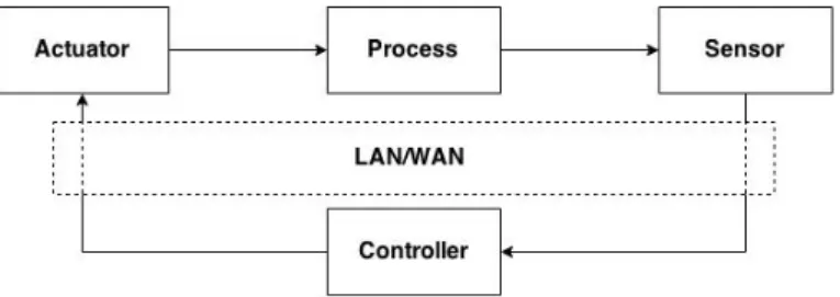
In our thesis the effect of adding a remote server to a closed control-loop needs to be investigated. A typical closed control-loop consists of a controller, an actuator, a sensor and a process to be controlled. As it can be seen in Figure4, the sensor produces a value by measuring the environment of the process and sends the information to the controller. The controller takes the measured value and, according to the desired output value, it computes a new output value. Afterwards, the controller feeds the output value to the actuator. The actuator makes the corresponding change on the process and after that the sensor can obtain an updated value.

Figure 4: Closed control loop

Our focus is the migration of the controller to remote servers. The system in Figure 4 is used as a reference model in the experiments. When a remote server is added in the control loop, latencies, jitter and packet loss can be introduced between the controller and the sensor or actuator. As Figure5 shows, the controller is connected to the actuator and the sensor via a network. The network can be either local (LAN) or global (WAN). For the former, the remote server is considered to be a local cloud (fog node) which resides close to the rest of the control loop. For the WAN case, the remote server is connected with the actuator and the sensor via internet, resulting in significant latencies between them.

Figure 5: Network Control System

4.2

Design

In this chapter the details of different hardware and software solutions used for developing the prototype are described.

4.2.1 System design

The system is based on existing hardware and software solutions. The Arduino starter kit7_{is used}

as the end device (the “thing”) to handle real-time tasks like a process automation system. The

starter kit includes Arduino Uno equipped with an ATMega3288_{microprocessor, prototype board,}

motors, sensors and LEDs. Arduino is a good choice for prototyping because there is a vast amount of libraries available online from serial port communication to more high-level communication such as Ethernet, IP stacks and TFT-LCD touch screens. A disadvantage of Arduino libraries is that they are not well documented. Arduino uses a C-based programming language and compiles with gcc9. Arduino is not made for process automation in practise because gcc is not meant for safety-critical systems [70], as it includes more than a 100 unpredicted cases, i.e., in some cases the compiler makes unpredicted compilation. In summary, the starter kit is a good choice for our purposes of fast prototyping but not the ideal for a real world machine. Building a back-end in real world machines is not possible due to limited time budget and to a more general approach of the subject.

The HP Compaq Elite 8300 Series computer is used as a server. It contains a i5-3470S quad-core Processor with a speed of 2.9 GHz and 3.7 GiB RAM. The server supports Intel’s virtual-ization technology (Intel VT-x) which minimizes the virtualvirtual-ization overhead for I/O and memory. Moreover, Intel VT enables virtual machines (VM) to run without performance degradation or compatibility issues, as if they were running natively on a CPU. Regarding memory, VT-x enables memory isolation and monitoring for each virtual machine separately. The server is approximately 600 time faster than the Arduino Uno which makes it good enough to be used as a server. The server runs a Ubuntu Server 14.04 LTS that hosts kernel virtual machines (KVM). The VM runs the Trusty distribution of Linux on a generic kernel.

As mentioned before, the network that connects the controller with the rest of the control loop can be either LAN or WAN. For the latter an emulator needs to be added to the system to introduce WAN characteristics such as delays, jitter and packet loss. For this purpose WANEM10 is utilized. WANEM is a software tool that can interfere with the incoming traffic and introduce the desirable network behaviour. WANEM can add delay, jitter packet loss, packet reordering, bandwidth limit, corruption, duplication and disconnection between nodes that are connected to it. WANEM is also able to add different rules for different routes in the network. In order to utilize WANEM one only needs to redirect the messages between nodes through the machine running WANEM.

WANEM runs on a virtual machine created with Oracles Virtual Box11 _{on Intel’s NUC} 12_.

Intel NUC is a small, really powerful computer that can use GPOS and high-level libraries as a normal personal computer. Intel NUC has various models available, most of which include i-series CPUs, DDR3 memories, USB, HDMI and Ethernet interface. Intel NUC can be used either to host a SDN real-time network or for fog computing because of its potential computation capabilities. Intel NUC is directly connected to Arduino, using Ethernet to maximize throughput. Since NUC can host a GPOS such as Linux or Windows, all the low-level libraries are already implemented in these OSs. The advantage of NUC is that it is expandable in certain ways and it can connect to HDD/SSD, USB3.0 and PCIe. Another advantage is that Intel is putting some effort in the IoT area, including the use of closed loops with gateways providing feedback to smart factories.

In order to implement the aforementioned design in a controlled environment, the schema of Figure6is used. All the components are connected to an Ethernet Switch (HP 1410-16G Switch13). When Internet needs to be added in the closed control loop, all the traffic from and to Arduino Uno is redirected and passed through WANEM. In the case of LAN, the Arduino Uno connects directly to the server. For all the experiments there are two different approaches for the control loop implementation which are two simple and initial ideas of how the control loop works when the controller is moved to a server. The first one, referred as polling, reads the sensor, sends the value to the server and waits until it gets the answer. Afterwards it applies the value and reads the sensor again. A descriptive pseudo code is provided in Algorithm1.

8_{http://www.atmel.com/products/microcontrollers/avr/megaavr.aspx} 9_{https://gcc.gnu.org/} 10_{http://wanem.sourceforge.net/} 11_{https://www.virtualbox.org/} 12_{http://www.intel.com/content/www/us/en/nuc/overview.html} 13_{http://h30094.www3.hp.com/product/sku/10256671/mfg partno/J9560A}

Algorithm 1 Polling

1: _{procedure Polling controller} 2: begin: 3: sensorValue ← readSensor(); 4: sendMsgToServer(sensorV alue); 5: loop: 6: if resultAvailable() then 7: result ← readResult(); 8: applyValue(result); 9: goto begin; 10: goto loop;

The second approach is the non-polling approach. The loop of this approach has three steps, the first step is to read the sensor, the second is to send the value to the server and the third is to check if there is a response from the server. If there is a response, the system reads the response and applies the value. If there is no response, the system moves to the first step. The pseudo code that describes the non-polling version is provided in Algorithm2.

Algorithm 2 Non-polling

1: _{procedure Non-polling controller} 2: begin: 3: sensorValue ← readSensor(); 4: sendMsgToServer(sensorV alue); 5: if resultAvailable() then 6: result ← readResult(); 7: applyValue(result); 8: goto begin;

The architecture to be evaluated includes a back-end machine connected to remote servers. Servers can be local, representing fog nodes or global and act as cloud servers. On the machine there is a closed control-loop that reads a sensor, computes a value according to the input and applies the result to an actuator. As shown in Figure4, the computation of the value is done locally on the machine. In our design we add the server to the closed control-loop. In this case, depicted in Figure 6, the machine sends the value to the server, the server computes the value and sends the computed value back to the machine and finally the machine applies the received value. Depending on where the server is in the network, latencies, jitter and even packet loss is introduced from the machine to the server and from the server to the machine. In the experiments there is no bandwidth limit.

Figure 6: Architecture overview

4.2.2 Delay mitigation mechanisms

Since the controller of the control loop is offloaded, and the control system influenced by network problems, it is of interest to have a local delay mitigation mechanism. Two different mitigation approaches are proposed here, one for each communication algorithm.

In order to improve the polling method, a timeout is introduced to stop the system for wait-ing forever on the server response and instead try and predict the misswait-ing server values. The timeout equals to the average round trip time (RTT) in the server communication. The RTT is the total time it takes a message to go from the client to the server and the server response to reach the client. Prediction methods are sometimes used in dynamic offloading to estimate changes in some parameters rather than checking every time. This includes predicting changes in parameters such as the load per node or available bandwidth, as is done in [71]. If the server does not respond in the expected time, the system predicts the value and uses that instead. The late responses from the server get buffered when they arrive and the system can either use those values when they arrive or disregard them. Both options are considered here, where applying the late values is labeled as buffering, and disregarding them is labeled as no buffering.

Two prediction models are used here: 1. Exponential moving average

2. Double exponential smoothing model

The exponential moving average [72] (also called exponential smoothing) is a simple weighted moving average of the data values and the previous statistic values. It is calculated as presented in equation (1), where stis the statistical value, st−1is the statistical value calculated in the previous

round, xt is the current observation and A is the smoothing factor. The smoothing factor, A, is

set between 0 and 1 and weights the data values.

st= Axt+ (1 − A)st−1 (1)

The current value st is an interpolation between the observation xt and the previous value

st − 1, where A determines how close the interpolated value is to the latest observation. The forecast for the next period is then the current value, as shown in equation (2)

Ft+1= st (2)

While the two prediction models mentioned are similar, the double exponential smoothing introduces another term that takes the change of the slope, or trend, into account. It is based

on the “Holt model” forecast [73]. The data value is calculated by the formula (3). In addition to the exponential moving average (see equation (1)), it has a parameter bt−1 that represents the

trend calculated in the previous round. The trend value is calculated in every round by using the equation (4). Apart from using the statistical data values st and st−1, as well as the previously

calculated trend bt−1, it also uses another smoothing factor B, set between 0 and 1. The first

smoothing factor, A, acts as a weight for the data values while the other one, B, weights the trend of the slope.

st= Axt+ (1 − A)(st−1+ bt−1) (3)

bt= B(st− st−1) + (1 − B)bt−1 (4)

The forecast can now be made for xt+m at the time

t + m, m > 0. The forecast is calculated as presented in equation (5)

Ft+m= st+ mbt (5)

Both methods depend on values from the previous round which doesn’t make it obvious how to start. There are a few different recommendations on how one can set the initial values, since not every approach works well for all cases. In our case, the initial values are set up based on the first values of the observation xt. In the case of the exponential moving average, the initial value

is

s1= x0,

while for the double exponential smoothing the initial values are s1= x0

b1= x1− x0.

Both methods also require setting the smoothing parameters, A and B, to a value between 0 and 1. While there is no formal way to do it, they can be calculated by using optimization techniques for getting the minimal error between the data and predicted values. In our case, the parameters are set using a trial and error method. Since having lower values of the A parameter means a slower response of the system, in our case higher values are preferred. The B parameter reflects how much change in the trend the model is expecting. A small value expects very little change and the other way around. In our case, the system works better for higher values of B since it adapts better to the rise of the curve in the beginning. The parameters in our system are set at A = 0.8 and B = 0.9. In order to improve the non-polling method, an adaptive PI controller is utilized. When the non-polling method is used and the delay increases more than the sampling period, the controller makes the decisions based on old messages because messages are queued in the network. Specif-ically, the controller’s sampling period is approximately 16 milliseconds (ms) thus the controller receives a new value every 16 ms. When the RTT is bigger than 16 ms, the controller sends a number of messages before it receives an answer. The number of messages sent before receiving an answer depends on the RTT. For example with 20 ms of RTT two messages are queued in the network. The result of the queued messages is to double the I part of the PI controller. Concretely, the integral part of the controller is computed by formula

integrali= integrali−1+ errori, f or i > 0,

where integral0= 0 and errori is the difference between the target value and the value read from

the sensor [74]. Therefore, when the first message is received from the controller the integral part is

Afterwards, the second message is received with the same sensor value, since as mentioned before the previous computed value has not applied yet. Therefore, for the second message we have error2= error1and so

integral2= integral1+ error2

= integral0+ 2 ∗ error1

= 2 ∗ error1

= 2 ∗ integral1.

From the last equation we conclude that for every queued message the integral part of the controller becomes a multiple of the initial value resulting in performance downgrade especially before the settling time. Settling time is the time elapsed to stabilize the output from a change of the input. On the other hand, the P part of the controller remains the same even when messages are queued in the network since it does not depend on previous values. In order to mitigate the ever increasing integral part of the PI controller, we apply a smoothing factor to the computed value of the controller. The actuator receives a value, applies the smoothing factor then applies the value to the plant. The smoothing factor is computed by the formula

a = sampling period sampling period + RT T

where RT T is the round trip time and sampling period is the sampling period that is used when the controller executes locally. The smoothing factor increases as the RTT increases. The smoothing factor applied is a type of adaptive controller but its definition is intuitive. Its benefits are examined by conducting a number of experiments in Section5.

4.3

End device set-up

The control loop consists of a photo-resistor (LDR-VT90N2) and an LED (LEDWC503B-WAN-CBADA151). The controller can change the brightness of the LED until it reaches the desired value. The LED values can be set between 0 and 1024, and the target value used in our experiments is 700. The sampling period is approximately 14 ms. In order to accomplish this a PI controller is utilized with proportional gain Kp= 0.001 and and integral gain Ki= 0.002. The Ziegler-Nichols

heuristic tuning method is used to obtain the initial values of the parameters and then manual fine tuning to obtain the final values. The Figure7illustrates the circuit diagram of the control-loop. As it can be noticed the LED is connected in series with a 330Ω resistor to a digital output of the microcontroller. Also the photo-resistor is connected in series with a 1kΩ resistor to a 5 Volts supply. The microcontroller reads the voltage drop across the photo-resistor through an analog input.

5

Experimental evaluation

This chapter contains the experiments that are conducted on the developed system. First we discuss the experimental setup. Then we discuss the results with constant and variable delays in the local controller. After that, an analysis of the delay mitigation mechanisms (the two prediction methods and the adaptive PI controller) is presented and compared to the local controller response under the same delays.

5.1

Experimental set-up

In the first set of experiments we investigate the effects of adding constant delays in the control-loop for both the polling and non-polling approaches. WANEM is used to inject the delays in the network. Firstly, the delays are set at 0, 1 and 10 ms, to investigate the effect of delays shorter than the sampling period in the control-loop, for both approaches. The second part of the first set of experiments is set to 50, 100 and 150 ms for the polling approach, and 15, 20 and 23 ms for the non-polling approach. The purpose of this set of experiments is to investigate the effect of delays longer than the sampling period to the control loop. In the second set of experiments, we investigate the effect of variable delays and jitter in the control-loop. WANEM is used to set the jitter to 1, 2, 5 and 10 ms for both approaches, in order to investigate the effect of small jitters in the control loop. Similarly, the second part of this set of experiments is to investigate the effect of jitter longer than the sampling period in the control loop. Jitter is set to 25, 50 and 75 ms for both approaches.

In the next two set of experiments, we apply the delay mitigation mechanisms, one for the polling method and one for the non-polling method. The second set of experiments uses the two prediction methods to test how they can improve the polling method. Both methods are tested under the delays and jitter that affect the control loop in the first set of experiments. The results are then compared between the two prediction methods and with the polling method without any prediction.

In the third set of experiments the Adaptive PI controller is used. The experiments target delays and jitters that exceed the sampling frequency. As mentioned earlier, the effect of delays smaller than the sampling period is not significant. Delays and jitter are set to the same values as in the first set of experiments in order to compare the results.

5.2

Local Response

In the first set of experiments, we investigate the effects of network latencies on the controller in both polling and non-polling approaches. In Figure8the controller is executed locally. As we can see the overshoot, the difference between the maximum value and the target value, is negligible and the settling time is 89 ms.

5.2.1 Constant delays

In the polling approach the latencies affect the sampling frequency of the control loop. In Figure9, three different communication latencies are examined. The direct communication with the server, labelled as fog, where the latency is less than half a millisecond and represents the communication with a local server where no latencies are introduced. In the other two cases, the latencies are set to 1 and 10 ms respectively. One can notice that the disturbance in the response curve is not big, especially for the fog and 1 millisecond communication latency. As expected, the delays that are less than the sampling frequency can be tolerated without significant change at the performance of the control loop. Therefore it can be concluded, that offloading the controller to local servers does not have any effect on the response.

Figure 9: Latency less than the initial sampling period

In Figure 10, the communication delays are more than the initial sampling period. In these three experiments the latency is dominating the control procedure and it is approximately 4, 8 and 12 times higher that the sampling period, respectively. It can be easily noticed that the disturbance is obvious, the overshoot is increasing and for 150 ms latency the system becomes unstable. The result is reasonable since controllers are tuned to work on a specific sampling frequency and make timely decisions.

Figure 10: Latency more than the initial sampling period

In Figure 11 the non-polling approach is used. As it can be noticed in this approach, when latencies are kept below the sampling period there is no great effect on the response. In the non-polling approach the degradation in the performance is severe when messages are queued in the network. As we can notice in Figure11, when the delay is 10 ms the controller sends two messages with the same value before it receives a response. This results doubling the I part of the PI controller and thus causes bigger changes to the actuator which downgrades systems’ performance. That is,

the system receives the first message, it computes a value and then it receives a second message with the same value. That makes the controller to compute a bigger value in order to decrease the error, since the previous value does not affect the system. Obviously, this interpretation from the controllers’ side is wrong since the first computed value has not applied yet.

Figure 11: Latency less than initial sampling period

In Figure 12, the fast degradation of the controller’s performance can be seen. When the latency is increased to 23 ms four messages are queued in the network. As a result, the system becomes unstable. The queued messages cause an increase in the I part of the controller before the computed value is applied. Additionally, the controller makes its decisions not on how the last computed value affects the system, but on how an older value affects the system. In this context, the age of the value is proportional to the network delays. Finally, as it can be derived from the figure below that the controller still stabilizes with 3 messages queued in the network.

Figure 12: Latency more than initial sampling period

5.2.2 Jitter

In the second set of experiments we investigate how jitter affects the performance of the controller. In Figure 13 the effect of four different values of jitter is depicted for the polling approach. As it can be noticed, the effect of jitter that is smaller than the sampling period does not affect the performance of the controller significantly. However, the jitter increases the overshoot but the system still manages to stabilize.

Figure 13: Jitter less than the initial sampling period for the polling approach

In Figure 14, it can be clearly seen that as the jitter increases and exceeds initial sampling period, the overshoot increases significantly. Additionally, one can notice the settling time increases and reaches, approximately, 600 ms. The performance of the controller is degraded and it cannot be considered acceptable compared to the local response characteristics.

Figure 14: Jitter more than the initial sampling period for the polling approach

In Figures 15 and 16, the performance of the non-polling approach for communication lines with jitter is investigated. As it can be clearly seen, the non-polling approach malfunctions when messages are queued in the network. Even if one message is queued in the network the degradation is considerable. Overshoot is more that 100 when one message is queued in the network and it rises fast as the jitter becomes bigger that the sampling period.

Figure 15: Jitter less than the initial sampling period for the non-polling approach

Figure 16: Jitter more than the initial sampling period for the non-polling approach

5.2.3 Discussion

By comparing the delays’ effect on the controller with the jitter, we can conclude that both affect the settling time since it takes more time to get enough responses to stabilize the system. Also, both the delay and jitter affect the overshoot of the controller. Additionally, the polling approach tolerates delays better than the non-polling approach. In the next four figures the changes of overshoot and settling time are depicted for the two approaches. Obviously the overshoot and the settling time for the non-polling approach increases faster as compared to the polling approach. Moreover, from the graphs we can verify that offloading the controller to fog nodes does not affect the system. Consequently, the local servers can be included in the control loop without performance degradation.

Figure 17: Overshoot using the polling approach

Figure 18: Overshoot using the non-polling approach

Figure 20: Settling time using the non-polling approach

5.3

Delay mitigation

In next set of experiments we try different methods to compensate delays and jitter in the control loop. The goal of the experiments, as said before, is to increase the reliability of the system when messages are delayed. For the polling approach, since messages are not received in every period, a prediction model is used, whereas in the non-polling approach a smoothing factor is applied to the received value to mitigate the ever-increasing computed value from the controller as a result of the queued messages.

5.3.1 Prediction methods

The prediction methods used here are, as mentioned before, the double exponential smoothing model and the exponential moving average. Both of them are applied in the polling method when the waiting time for the server exceeds a timeout of 18ms, as that is the average RTT between the device and the server. The communication between the server and the device is capable of buffering the messages between them. In the case of higher delays the buffered messages become older and older as the system continues to use them. But if the system does not buffer the messages then it makes use of less values form the server in total. The prediction methods, however, depend on being updated with new values. Both prediction models are tested with and without buffering the messages. The tests show that buffering and not buffering gives similar results in the lower delays, but not buffering takes more time on the same number of samples, since it reaches the timeout more often than buffering. In the case of tests with constant delays, for the double exponential smoothing the not buffering approach starts to become unstable at 75ms delay (see Figure21). For the exponential moving average the curve also loses its smoothness at 75ms delay (see Figure22). This is because both of these methods start using more predicted than calculated control values at this point, around 65.68%. In the case of tests with variable delays, the no buffering approach gives results that are very close to the buffering approach, but still uses more predicted values and takes longer time. In the analysis presented from here on, only the buffering method is considered.