Representing travel cost variation in large-scale models of long-distance passenger transport

www.transportekonomi.org

Representing travel cost variation in large-scale models

of long-distance passenger transport

Ida Kristoffersson, VTI

Andrew Daly, Leeds University

Staffan Algers, TPMod

Stehn Svalgård-Jarcem, WSP Advisory

Working Papers in Transport Economics 2020:6

Abstract

In this paper we show that travel cost variation for long-distance travel is often substantial, even within a given mode, and we discuss why it is likely to increase further in the future. Thus, the current praxis in large-scale models to set one single travel cost for a combination of origin, destination, mode, and purpose, has potential for improvement. To tackle this issue, we develop ways of accounting for cost variation in model estimation and forecasting. For public transport, two methods are developed, where the first method focuses on improving the average fare, whereas the second method incorporates a submodel for choice of fare alternative within a demand model structure. Only the second method is consistent with random utility theory. For car, cost variation is related to long run decisions such as car type choice and employment location. Handling car cost variation therefore implies considering car type choice and workplace choice rather than different options related to a specific trip. These long-term choices can be considered using a car fleet model.

Keywords

1. Introduction

Large-scale transport models of long-distance passenger transport are often used in cost-benefit calculations of infrastructure investments or policy implementations. One common application of such a model is to investigate the costs and benefits of building high-speed rail (Cambridge Systematics 2016; WSP 2011). The electric vehicle market is developing (Liu and Lin 2017; Jensen et al. 2017) and thus another application, likely to be more common in the near future, is to analyse the effects of electrification of the car fleet on long-distance travel. Both high-speed rail and electric cars form new cost alternatives for future long-distance travel. One core feature of large-scale transport models is therefore the way travel costs are represented in the model. For public transport (PT) modes such as rail, air, and long-distance bus, this refers to the representation of fares, whereas for car this refers to the representation of fuel and other operational costs in the model.

Typically, in large-scale modelling of public transport cost, a single average fare is used for one combination of origin, destination, mode, and trip purpose (typically private or business). Sometimes the fare implemented in the model differs also by person type (e.g. commuters might be assigned season tickets). Long-distance models that include submodels of the choice of different travel fares are scarce. Models exist, such as PRAISE in the UK (Whelan and Johnson 2004), which do model this choice, but they have a much more restricted scope compared to national large-scale travel models. However, large variation exists in travel costs both for PT modes and for car. Dynamic pricing strategies have increased, and rail and air operators often use revenue management strategies to adjust fares to actual demand and customer heterogeneity (Hetrakul and Cirillo 2015). The opening of the rail market for competition between different operators has also had an effect on ticket prices for example in Sweden (Vigren 2017).

For car, the introduction of electric vehicles will likely increase travel cost variation further from a situation already differentiated by differences in car size, fuel type and fuel efficiency. The

appropriate cost of driving a car that should be entered into model estimations or applications is not easy to state simply. Among the issues that need to be considered are:

• to what extent the ownership costs, i.e. the costs that are incurred whether or not the car is driven (e.g. most of the depreciation and insurance costs), should be included.

• how choices made by the owner or driver, such as the type of car or fuel and the driving style (e.g. speed choice), need to be taken into account.

• how taxation is accounted.

• how compensation, in particular by an employer, is included.

A useful text and recommendations on these issues can be found in the UK government’s Transport Analysis Guidance, called TAG or WebTAG (Department for Transport 2019). This approach is based on an attempt to calculate the marginal cost per kilometre to the owner or driver. The cost is based on a very detailed calculation of fuel consumption per kilometre which is intended to be an average for the UK vehicle fleet of vehicle efficiency and fuel type; forecasts of changes in efficiency and fuel type are also given. The WebTAG methodology for calculating car driving costs is used in many large-scale models, for example models for Manchester (RAND Europe 2013) and West Midlands (RAND Europe 2014). The method used in the Swedish long-distance model is similar to WebTAG with a detailed calculation of fuel consumption per kilometre, which is intended to be an average for the Swedish

vehicle fleet. One difference is that car costs for business trips are assumed equal to private trips in the Swedish model, whereas this is not the case in the UK guidelines.

In this paper we show that travel cost variation for contemporary domestic long-distance travel is substantial and discuss why it is likely to increase further in the future. Furthermore, we suggest ways of accounting for cost variation in model estimation and forecasting.

2. Example of contemporary travel cost variation for long-distance trips

2.1 Overview of long-distance travel in Sweden

2.1.1 Context

Sweden is a geographically extended country with about 1570 km from the southernmost to the northernmost point. Domestic long-distance travel is therefore quite common and has also been reinforced by a strong urbanisation trend past decades, spreading family generations over the country. The Swedish travel survey from 2011-2016 shows that as much as 74 % of long-distance trips are private trips with different purposes such as visiting family and friends, whereas only 14 % are business trips (Berglund and Kristoffersson 2020). The most common travel modes for domestic long-distance travel within Sweden are car (73 %), train (16 %), air (5 %), and long-distance bus (4.5 %). Modal shares depend a lot on trip purpose, e.g. with train and air shares being substantially larger for business trips. In many ways, Sweden is typical of a European country, wherefore the considerable diversity in travel costs and the discussion on how to account for this diversity is likely to be applicable also to other countries. Of course, discussion related to air travel is not relevant for smaller countries where domestic travel is not conducted by air.

2.1.2 Public transport

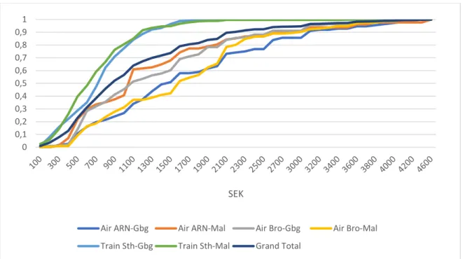
Figure 1 shows that there is substantial travel cost variation for long-distance public transport even when fares are segmented by mode, OD pair and route. The data set used is a stated preference (SP) data set related to high-speed rail modelling (WSP 2011). Fare distributions are segmented by the modes train and air, the OD pairs Stockholm-Gothenburg and Stockholm-Malmö (the two main OD-pairs for long-distance travel in Sweden, since it involves the three largest cities in Sweden), and the routes Arlanda-Gothenburg, Arlanda-Malmö, Bromma-Gothenburg, and Bromma-Malmö (dividing air travel from Stockholm into the two main airports Arlanda and Bromma).

Figure 1: Cumulative fare distributions within each mode (train or air), OD pair (Gothenburg and Stockholm-Malmö) and route (separating Bromma Airport (Bro) from Arlanda Airport (ARN)). Travel costs are given in SEK1_.

The fare distributions for train are similar, one reason being that the same operator runs the service. The distributions are also not as wide as for air, as train tickets are cheaper in general.

Figure 2 shows the distribution of ticket prices for the air route Stockholm-Arlanda to Gothenburg, to better show the frequency of each fare class. The average fare is 1638 SEK, but the fare variation is large as is shown in the figure.

Figure 2: Distribution of ticket prices for air travel between Arlanda in Stockholm (ARN) and Gothenburg (Gbg).

1 _{10 SEK ≈ 1 EUR} 0 0,1 0,2 0,3 0,4 0,5 0,6 0,7 0,8 0,9 1 SEK

Air ARN-Gbg Air ARN-Mal Air Bro-Gbg Air Bro-Mal Train Sth-Gbg Train Sth-Mal Grand Total

0 0,02 0,04 0,06 0,08 0,1 0,12

Air ARN-Gbg

2.1.3 Car

Somewhat more surprisingly there is considerable variation also in car travel costs, see Figure 3. Calculations are based on data from the Swedish car register containing fuel consumption for cars from years 2000 – 2014. Unfortunately, data on the marginal cost of car travel other than fuel costs has not been available to the project. The fuel consumption data base reflects the passenger car fleet composition in early January 2015. The number of vehicles in the data base includes 3 395 000 active cars registered in the 2000 – 2014 period. For each car in the database, fuel consumption per 100 km is multiplied by the fuel cost for each fuel type (petrol, diesel, electricity) as of 2014, see Table 1. The reader should keep in mind that petrol and diesel prices vary, which obviously may have an impact on the cost distribution. However, the correlation between petrol and diesel prices is very high, so this would affect the distribution mean rather than the variance. The price of electricity of 1.1 SEK/kWh in Table 1 is calculated based on the assumption that the electric cars are charged at home. For long distance travel however, charging often needs to be done at public charging stations, where prices are much higher, up to 3 times higher than for home charging. For plug-in hybrids, range is quite important, as it also affects fuel type. The electric range for plug-in hybrids is often less than 50 km, implying that longer distance trips mostly will use petrol rather than electricity. Petrol

consumption for plug-in hybrids may be quite high in many cases.

Table 1: Fuel costs in December 2014 in SEK per litre/kWh.

Petrol Diesel Electricity

14.32 14.19 1.1

Figure 3: Fuel cost distribution for Swedish cars of model year 2000-2014.

0% 2% 4% 6% 8% 10% 12% 14% 16% 18% 20% 5 15 25 35 45 55 65 75 85 95 105 115 125 135 145 155 165 175 185 195 205 SEK per 100 km

Figure 4 shows the fuel cost distribution for the OD-pair Stockholm-Gothenburg. Comparing with Figure 1 one can conclude that the car cost variation is of the same magnitude as the variation for train travel, given that there is only one person in the car. Larger party sizes lead to less variation in absolute terms.

Figure 4: Fuel cost distribution for cars with model year 2000-2014 for the trip Stockholm – Gothenburg.

So far, what has been discussed is variation in vehicle costs, but for business trips, car travel costs are often not equal to the vehicle costs. Business travellers are compensated for their car travel with reimbursement and the level of reimbursement varies a lot. WSP (2016) shows that the

reimbursement for travellers who used their private car for a business trip in Sweden in 2015 varied between 13 and 44 SEK per 10 km. The typical reimbursement is SEK 18.50, which is at present the maximum amount allowed without having to pay a benefit tax, but about half of car users got more than this amount. Also for company benefit car users the compensation for fuel costs varied between 2 and 55 SEK per 10 km in 2015 (WSP 2016).

2.2 Explanatory factors for contemporary travel cost variation

2.2.1 Public transport

Analysis of the data shows that the remaining cost variation (after segmentation by mode, OD pair and route) is partially explicable by ticket type, departure time in peak and income for air travel, and by ticket type, senior citizenship, and income for train travel, see Table 2 and Table 3 for results of the regression analysis these inferences are based upon.

Table 2 shows that the ticket type variables (FullFlex and Flex, but not FixEconomy), as well as the departure time in peak variable (Peak) are significantly different from zero and give significant contributions to the fare paid. These effects remain also when additional variables are included. The route effect for Stockholm-Gothenburg (RouteSG), implemented as a dummy which is one if the route is Arlanda-Gothenburg, and the operator effect included as a dummy for SAS as operator (OPSAS), are not significant. Age effects (Age65+ and Age-27) are also not significant, but income effects are (Inc-20 and Inc40+). As can be expected, travellers with income less than 20 000 SEK per month choose cheaper tickets, and travellers with income more than 40 000 SEK per month choose

0% 2% 4% 6% 8% 10% 12% 14% 16% 18% 20% 24 72 120 168 216 264 312 360 408 456 504 552 600 648 696 744 792 840 888 936 984 SEK Sthlm - Gbg

more expensive tickets. The gender variable (GenderW), which is one if the traveller is female, is not as significant as the ticket type and departure time in peak variables. When introducing the gender variable, the low-income variable becomes insignificant, probably because of a correlation between income and gender.

Table 2: Regression models of air traveller fares.

Model 1 Model 2 Model 3 Model 4

Variable Parameter t-value Parameter t-value Parameter t-value Parameter t-value

GenderW -179.4 -1.9 Inc40+ 271.8 2.9 222.9 2.3 Inc-20 -375.0 -2.3 -306.3 -1.8 Age65+ -275.2 -1.2 -230.5 -1.0 -222.4 -1.0 Age-27 -195.2 -1.3 16.4 0.1 10.1 0.1 OPSAS 178.4 1.6 189.0 1.7 166.9 1.6 131.1 1.2 RouteSG 37.2 0.4 35.9 0.4 -15.4 -0.2 -18.5 -0.2 FullFlex 1021.4 7.0 975.9 6.5 832.5 5.6 806.1 5.4 Flex 680.7 5.2 623.2 4.6 528.1 3.9 541.1 4.1 FixEconomy 17.4 0.2 -22.6 -0.2 -88.4 -0.8 -85.6 -0.7 Peak 363.9 3.7 333.5 3.4 353.6 3.7 356.2 3.8 Intercept 678.1 5.8 764.3 6.0 750.4 5.7 856.8 6.0 r2 0.36 0.37 0.42 0.43

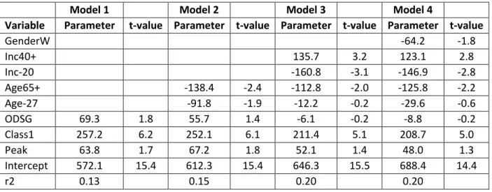
In Table 3, the corresponding regression models for train is shown. Table 3 shows that for train, the first-class ticket type variable (Class1) is significantly different from zero, whereas the dummy for OD pair Stockholm-Gothenburg (ODSG) and the departure time in peak (Peak) variables are not. When age is added, the effect for the group 65+ (Age65+) also turns out to be significant, whereas that for the group under 27 years (Age-27) does not. Income effects (Inc-20 and Inc40+) also appear as significant, while the gender effect (GenderW) is marginal.

Table 3: Regression models of train traveller fares.

Model 1 Model 2 Model 3 Model 4

Variable Parameter t-value Parameter t-value Parameter t-value Parameter t-value

GenderW -64.2 -1.8 Inc40+ 135.7 3.2 123.1 2.8 Inc-20 -160.8 -3.1 -146.9 -2.8 Age65+ -138.4 -2.4 -112.8 -2.0 -125.8 -2.2 Age-27 -91.8 -1.9 -12.2 -0.2 -29.6 -0.6 ODSG 69.3 1.8 55.7 1.4 -6.1 -0.2 -8.8 -0.2 Class1 257.2 6.2 252.1 6.1 211.4 5.1 208.7 5.0 Peak 63.8 1.7 67.2 1.8 52.1 1.4 48.0 1.3 Intercept 572.1 15.4 612.3 15.4 646.3 15.5 688.4 14.4 r2 0.13 0.15 0.20 0.20

2.2.2 Car

The analysis of fuel cost variation shows that the main explanatory factors for fuel cost variation are

fuel type, fuel efficiency and model year. These factors are correlated, as fuel type and fuel efficiency

are both dependent on model year. Diesel cars have become more common in Sweden during the latest years, and electricity is starting to gain ground. Furthermore, newer cars are in general more fuel efficient compared to older cars. These changes in the Swedish car fleet over the years are partly caused by a number of car fleet policy measures.

Figure 5 shows that Diesel cars are in general cheaper per 100 kilometres than Petrol cars. This is slightly due to difference in fuel cost per litre (see Table 1) but mainly due to Diesel cars being more fuel efficient. Electric cars are too few to give a visible effect in the figure, but they are cheaper than most Diesel and Petrol cars per 100 kilometres.

Figure 5: Fuel cost distribution for Swedish cars of model year 2000-2014 segmented by fuel type.

0% 2% 4% 6% 8% 10% 12% 14% 16% 18% 20% 5 15 25 35 45 55 65 75 85 95 105 115 125 135 145 155 165 175 185 195 205 SEK per 100 km Petrol Diesel El

Figure 6 shows the fuel cost distribution for cars of model year 2000, 2006, and 2014, respectively. It is clear that the fuel cost distribution shifts to the left as years pass by, i.e. fuel costs decrease. This decrease in fuel costs is mainly driven by cars becoming more and more fuel efficient.

Figure 6: Fuel cost distribution for Swedish cars of model year 2000, 2006, and 2014, respectively.

Fuel cost can be expected to vary more in the future, because of the expected growth of electric vehicles having considerably lower fuel costs compared to conventional vehicles. This growth will be specifically driven also by European and national climate policies. On the other hand, policy

measures to ensure that marginal costs for car travel are internalised might be implemented in the future. These would likely be higher in congested areas (and during congested times) and would therefore be expected to affect urban travel to a higher degree than long-distance travel.

0,% 5,% 10,% 15,% 20,% 25,% 30,% 5 15 25 35 45 55 65 75 85 95 105 115 125 135 145 155 165 175 185 195 205 SEK per 100 km 2014 2006 2000

3. Methods to Account for Cost Variation in Model Estimation and Forecasting

3.1 Public transport

The typical implementation of public transport costs in large-scale models is to use one average fare per mode, OD, and trip purpose. This approach does not capture existing cost variation and may even result in counter-intuitive results, since an improvement in the offer, e.g. a reduction in the first-class fare, may lead to an overall decrease in the utility for train, if enough people change fare alternative and the overall average price increases. Another example is when there is, for a given journey, one fast and one slow service and a higher fare applies to the faster service. Then if the fare for the faster service is reduced somewhat, but not to the level of the slower service, some more travellers will use the fast service. What happens to the average fare? Those who were already using the fast service will pay less, but those who switch will pay more, and it is quite possible that the average fare will increase. Since no other aspect of the service has changed, this will imply that the overall rail service is less attractive, and a large-scale model will predict a switch away from train travel. The reason for the outcome of both examples above is that the average fare is not consistent with random utility theory. We now describe two ways to better capture cost variation in model estimation and forecasting. Only the second method is consistent with random utility theory.

3.1.1 Improving the average fare

Using the first method, the public transport average fare calculation is improved by segmenting the fare into an increased number of fare categories and using data on the distribution of travellers over these fare categories.

The average fare is calculated by

𝑓̅ = ∑ 𝑝𝑗 𝑗. 𝑓𝑗 (1)

where 𝑝𝑗 is the share of travellers choosing fare category 𝑗 and

𝑓𝑗 is the fare for category 𝑗.

The improvement in cost representation using this method lies in the extended description of the travel fares that exist and the use of more detailed data on traveller distribution over these fare categories.

The implementation of segmentation over different fare categories requires path choice to be made for each fare category, using available public transport assignment software, to calculate level of service variables for that specific fare category. If the fare varies by route, then assignment need to take into account also variation by person type, covering both the availability of some fare types to specific person types and the variation of the value of time in the population.

The distribution of travellers over fare categories may change in future, so that the average fare may change without any change in the prices of tickets. While the changes in the coming 20 years in the split over different public transport fare categories are not expected to be as large as the changes in split over different car fuel types, accurate forecasting also requires these shares to be forecast.

3.1.2 Submodel for choice of fare alternative

In the second method, we propose to use the logsum from a multi-fare choice model in mode-destination choice forecasting, to be consistent with random utility theory. The fundamental problem with the use of average fare as a composite fare measure is that the average is not consistent with a utility basis for the model. If the fare of an alternative is increased, the utility of that alternative is

reduced, and we also expect that the utility for the whole set of alternatives should be reduced. The issue is how the composite utility for the set of alternatives is calculated for input to the mode-destination modelling and to specify the role of fares in that composite utility. It has long been known that, if choice for a set of alternatives is modelled using a logit model, then the only utility-consistent measure of composite utility for the set of alternatives is the logsum 𝐿, and is defined by

𝐿 = log(∑_𝑖

exp 𝑉

Where 𝑉𝑖 is the utility of alternative 𝑖 , usually a linear function of the fare and other attributes.

This is clearly not the same as the average utility, which is calculated by

𝑉̅ = ∑𝑖

𝑝

𝑉

To see how these are related, consider the logarithmic form of the logit model:

log

𝑝

𝑉

log(∑

exp 𝑉

= 𝑉

If we multiply equation (4) by 𝑝𝑗 and add up over all the alternatives, we obtain, since the probabilities

add up to 1

∑_𝑗

𝑝

𝑝

𝑝

𝑉

−

𝑝

𝐿

= 𝑉

Reformulation of equation (5) leads to:

𝐿 = 𝑉̅ − ∑ 𝑝𝑗 𝑗log 𝑝𝑗 = 𝑉̅ + 𝐸 (6)

That is, because all the log probabilities are negative, the logsum is larger than the average utility. The positive difference, (− ∑_𝑗

𝑝

𝑝

in transport planning for many years, although it has largely been replaced by utility theory.

The key feature of the logsum in the present context is that it responds correctly to fare changes, specifically

𝜕𝐿

𝜕𝑓_𝑘

= 𝑝

𝛽

where 𝛽𝑓 is the coefficient of the fare in the linear utility function 𝑉𝑘. This always has the correct

(negative) sign and retains consistency with the utility theory underlying the model.

2 _{In statistical mechanics, for example, the “entropy is a logarithmic measure of the number of states with}

significant probability of being occupied” (Wikipedia, which goes on to give the formula of equation (6)). In information theory, this measure is defined as Shannon entropy.

The advantage of this formulation is that we can now use the average fare (and average travel time etc.) in calculating 𝑉̅. In fact, this calculation is exactly what would be done if we were to use the averages for these variables. All that must be done is to add the entropy to the utility.

In calculating entropy, we note that all that is required is the probabilities for each alternative. Some means must be found to forecast these, but this must be done in any case to calculate the average for the fare and other variables. This step is identical to the step of calculating traveller shares for the different fare categories in the first method described in the previous section.

The scale of equation (6) needs consideration. It would be usual to expect that the scale of choice among ticket types, routes etc. would be higher than the scale in the mode-destination choice model, i.e. the sensitivity of travellers’ choices to utility would be greater for within-mode switching than for between-mode switching, so that a scaling needs to be applied to between-mode choice, often designated by 𝜃, with 0 < 𝜃 ≤ 1. The coefficients within 𝑉̅ have been estimated at mode-destination level, i.e. the scaling by 𝜃 is implicit, so that what is required is to add 𝜃𝐸 to the

calculated mean utility. Estimation of 𝜃 requires some additional investigation. We would then arrive at a revised version of equation (6):

𝜃𝐿 = 𝑉̅∗_{+ 𝜃𝐸 (8)}

where 𝑉̅∗ is the mean utility as currently used in the mode-destination modelling, with the scale defined for those choices, which is likely to be smaller than the scale defined for within-mode choices.

Care is needed in practice. Experience has shown that the impact of 𝐸 can be excessive, particularly when the number of alternatives changes. The extreme case is when a new alternative is introduced which has the same overall utility as a single existing alternative. The entropy changes from 0 to log 2, which is approximately 0.69, while the average utility does not change. In models of long-distance choice, where the coefficients are relatively small, the value 0.69 can represent many minutes of travel time, so that a careful calculation of 𝜃 is essential and the assumption that 𝜃 = 1 (as might be a naïve expectation) can cause difficulty.

We conclude that it is feasible to use this alternative approach, to avoid basing the model entirely on averages of fare (and other variables). However, this introduces some complications in programming the addition of entropy to the utility functions and in estimating the parameter 𝜃.

3.2 Car

As is discussed in section 0, there are expected to be considerable differences in marginal cost between electric, hybrid and internal combustion (i.e. petrol and diesel) cars. Determining an average car cost therefore requires a good estimate of the split over fuel types, as well as forecasts of the costs of each fuel type. Moreover, the costs of electric cars may depend on tour lengths, particularly for long tours, which are the key focus of this study. These costs depend on technological developments and government policy, while the split further depends on traveller choices and the rate of incorporation of electric vehicles into the fleet. Car fuel cost variation is a different type of cost variation compared to public transport cost variation. For car, the variation is related to long run decisions like car type choice and employment location, whereas public transport cost variation is related to specific trips. Handling car fuel cost variation therefore implies considering car type choice and workplace choice rather than different options related to a specific trip.

It is easy to establish a base year car fuel cost distribution based on the Swedish car register. To be useful for forecasts, this distribution must be forecast as well. To do this, a car fleet model is needed.

In 2006, such a model for Sweden was developed for the Swedish Road Administration. The Swedish car fleet model is a cohort-based model, where the base year car fleet is propagated year by year considering scrapping, car ownership level and addition of new cars. The demand for number of new cars is defined by the difference between the number of cars implied by the forecast car ownership level and the car fleet size after scrapping. The distribution of new cars by fuel type and fuel

consumption is calculated using a discrete choice model. An earlier version of the model has been described in Beser Hugosson et al (2016) and in Habibi et al (2019). A recent version has been described in Engström et al (2019). The model has also been used by Swedish planning authorities, the most recent application being for the Swedish Environmental Protection Agency 2017 (TPmod AB 2017).

The car fleet model output is currently quite aggregate but can easily be modified to also produce a distribution of car fuel cost per km, consistent with the car fleet input data. The distribution can then be used in two different ways. The simplest is of course to use the mean or the median of the distribution as car fuel cost in the mode-destination choice model. A more elaborate way would be to use the distribution as such, which would require the mode-destination choice model to be based on microsimulation (simulating behaviour by individuals rather than groups of individuals). In a microsimulation setting, each individual would be assigned a specific car from the total distribution of cars. Currently the car choice model operates at the national level, which means that no

geographical variation is considered. Considering regional variation would require a regionalisation of the model, which would also be necessary for analysis of geographically differentiated car fleet policies.

The variation in reimbursement for business trips can be accounted for when calculating car travel costs in the model. Currently, reimbursements are not explicitly considered at all in the Swedish long-distance model and is therefore implicitly accounted for in the cost coefficient of the model. It should be noted that this is not ideal from a model estimation point of view if the cost coefficient is

constrained to be the same for all modes, which is the case for the business model. In such cases it is important that all costs are included. One suggestion is to use the tax authority maximum amount allowed without having to pay a benefit tax for a certain share (from data) of the car users and an average for car users getting a different reimbursement. This method would apply both to travellers using their private car for business travel and to company benefit car users paying fuel costs

privately, even though the shares and average reimbursements would differ between the two categories.

4. Discussion

In this paper it is shown that travel costs for long-distance trips vary significantly for both car and public transport (train and air) for the Swedish case. Given that the air and rail market have opened up for competition in many countries in Europe, Sweden is likely a representative case. Even though cost variation is substantial, and travel cost is one of the most important input data when using large-scale models to conduct cost-benefit analyses of major transport projects, cost, and especially cost variation, is inadequately represented in most large-scale systems of long-distance trips. More focus and scientific effort have traditionally been put on the demand modelling side, i.e. the estimation of behavioural parameters for mode and destination choice. This is unfortunate, for example since deficiencies in cost data will also affect the cost parameter estimates, and in turn the value of travel time.

For large-scale transport modelling systems in Europe, we find that somewhat more effort has been put into the modelling of car cost variation compared to public transport cost variation. In several cases, car fleet models are used to model the composition of different fuel types and fuel

consumption levels in the national car fleet, both at present and for the forecast year. Furthermore, the calculation methodology is often well documented and easy to follow. However, there is room for some improvement also for car cost calculations. The detailed data from car fleet models already used could be utilised better. Given mode and destination choice models in which a synthetic population is used, then the full car cost variation could be modelled by making draws from the car fleet and assigning one specific car to each car-user in the synthetic population.

Cost modelling for public transport trips has even larger potential for improvement. Most large-scale models refer to unpublished reports when discussing the costs that are used for public transport long-distance travel. A more transparent process and documentation of public transport travel costs would be beneficial to the overall development of large-scale modelling. Furthermore, we show in this paper that the current praxis of using one average fare per mode, OD pair and trip purpose, is not consistent with utility theory if several fare alternatives are available to the traveller, e.g. depending on service, route or ticket category. In this case, an improvement in the offer to the traveller might lead to an overall decrease in the utility for that mode. In this paper we show that this problem can be overcome by introducing a logit fare choice model and using the logsum from the fare choice model in the mode and destination choice model. We also show that this logsum is composed of the average fare plus a term called entropy, which is related to the switching of fare alternatives. When implementing such a fare choice model, one need also to include a scaling factor for the entropy, since travellers usually switch more easily between different fare alternatives, compared to changing mode or destination.

Acknowledgement

This work was conducted within the Primo project funded by the Swedish Transport Administration under Grant TRV 2019/11943.

References

Berglund, Svante, and Ida Kristoffersson. 2020. ‘Anslutningsresor: En Deskriptiv Analys (Connection Trips: A Descriptive Analysis)’. 2020:3. Working Papers in TransportEconomics.

https://www.diva-portal.org/smash/get/diva2:1416370/FULLTEXT01.pdf.

Beser Hugosson, Muriel, Staffan Algers, Shiva Habibi, and Pia Sundbergh. 2016. ‘Evaluation of the Swedish Car Fleet Model Using Recent Applications’. Transport Policy 49: 30–40.

Cambridge Systematics. 2016. ‘California High-Speed Rail Ridership and Revenue Model’.

https://www.hsr.ca.gov/docs/about/ridership/CHSR_Ridership_and_Revenue_Model_BP_M odel_V3_Model_Doc.pdf.

Department for Transport. 2019. ‘TAG UNIT A1.3 - User and Provider Impacts’.

https://assets.publishing.service.gov.uk/government/uploads/system/uploads/attachment_ data/file/805260/tag-unit-a1-3-user-and-provider-impacts.pdf.

Engström, Emma, Staffan Algers, and Muriel Beser Hugosson. 2019. ‘The Choice of New Private and Benefit Cars vs. Climate and Transportation Policy in Sweden’. Transportation Research Part

D: Transport and Environment 69: 276–292.

Habibi, Shiva, Muriel Beser Hugosson, Pia Sundbergh, and Staffan Algers. 2019. ‘Car Fleet Policy Evaluation: The Case of Bonus-Malus Schemes in Sweden’. International Journal of

Sustainable Transportation 13 (1): 51–64.

Hetrakul, Pratt, and Cinzia Cirillo. 2015. ‘Customer Heterogeneity in Revenue Management for Railway Services’. Journal of Revenue and Pricing Management 14 (1): 28–49.

Jensen, Anders F., Elisabetta Cherchi, Stefan L. Mabit, and Juan de Dios Ortúzar. 2017. ‘Predicting the Potential Market for Electric Vehicles’. Transportation Science 51 (2): 427–440.

Liu, Changzheng, and Zhenhong Lin. 2017. ‘How Uncertain Is the Future of Electric Vehicle Market: Results from Monte Carlo Simulations Using a Nested Logit Model’. International Journal of

Sustainable Transportation 11 (4): 237–247.

RAND Europe. 2013. ‘Manchester Motorway Box - Post-Survey Research of Induced Traffic Effects’. TR676. https://www.rand.org/pubs/technical_reports/TR676.html.

———. 2014. ‘PRISM 2011 Base - Mode-Destination Model Estimation’. RR186. https://www.rand.org/pubs/research_reports/RR186.html.

TPmod AB. 2017. ‘Bilparkens Utveckling 2017 –2030 Med Hänsyn till Nya Styrmedel - En Simuleringsstudie’. Report TPmod (in Swedish).

Vigren, Andreas. 2017. ‘Competition in Swedish Passenger Railway: Entry in an Open Access Market and Its Effect on Prices’. Economics of Transportation 11: 49–59.

Whelan, Gerard, and Daniel Johnson. 2004. ‘Modelling the Impact of Alternative Fare Structures on Train Overcrowding’. International Journal of Transport Management 2 (1): 51–58.

WSP. 2011. ‘Höghastighetståg - Modellutveckling, Forskningsrapport (High Speed Train - Model Development, Research Report)’.

http://fudinfo.trafikverket.se/fudinfoexternwebb/Publikationer/Publikationer_001401_0015 00/Publikation_001404/HHT%20rapport_110622.pdf.

———. 2016. ‘Val Av Förmånsbil - Förmånsbeskattning, Företagspolicy Och Konsumentpreferenser’. FUD-rapport.

https://www.trafikverket.se/contentassets/773857bcf506430a880a79f76195a080/forskning sresultat/val_av_formansbil_formanbeskattning_foretagspolicy_och_konsumentpreferenser. pdf.