2003:41 Development of a Quantitative Framework for Regulatory Risk Assessments: Probabilistic Approaches

SKI Report 2003:41

SSI report 2003:19

Research

Development of a Quantitative Framework

for Regulatory Risk Assessments:

Probabilistic Approaches

R. D. Wilmot

November 2003

ISSN 1104-1374 ISSN 0282-4434

SKI/SSI perspective

Background

SSI has issued regulations that impose a risk criterion for radioactive waste disposal. SKI has issued corresponding regulations on long-term safety of geological disposal, including aspects and guidance on safety assessment methodology (such as time frames). Based on these regulations, SSI and SKI need to develop an attuned view of what is expected from the applicant, in terms of risk assessment in support of a license application. A previous study for this purpose (SKI ref. no. 14.9-010580/01114 and SSI ref. No. 60/2760/01, SSI P 1288.01) provided qualitative descriptions of various approaches to risk assessment by reference to assessments in other countries.

Relevance for SKI & SSI

One approach to evaluate risk in performance assessments is to use probabilistic

approaches to express uncertainties. This report describes the various approaches available for undertaking such probabilistic analyses, both as a means of accounting for uncertainty in the determination of risk and more generally as a means of sensitivity and uncertainty analysis. Also the use of different outputs for presenting probabilistic results is discussed in the report, since communication of results constitutes an important part of an assessment. In addition, the report describes issues that must be considered when characterising and interpreting risk and dose as a function of time.

Results

The objective of this project has been fulfilled. The current project is intended to build upon the previous study and to provide additional support to SSI’s and SKI’s

understanding of risk and how it can be treated in assessments. The specific objective was to review available probabilistic techniques to account for uncertainties, both regarding description of the mathematical basis for different techniques and to survey how different techniques have been used in practise.

Project information

SKI project manager: Eva Simic

Project Identification Number: 14.9-020495/02267 SSI project manager: Björn Dverstorp

SKI Report 2003:41

SSI report 2003:19

Research

Development of a Quantitative Framework

for Regulatory Risk Assessments:

Probabilistic Approaches

R. D. Wilmot

Galson Sciences LTD

5 Grosvenor House

Melton Road

Oakham

Rutland LE15 6AX

United Kingdom

November 2003

This report concerns a study which has been conducted for the Swedish Nuclear Power Inspectorate (SKI) and the Swedish Radiation Protection Authority (SSI). The conclusions and viewpoints presented in the report are those of the author/authors

iii

Executive Summary

The Swedish regulators have been active in the field of performance assessment for many years and have developed sophisticated approaches to the development of scenarios and other aspects of assessments. These assessments have generally used dose as the assessment end-point and have been based on deterministic calculations. Recently introduced Swedish regulations [SSI FS 1998:1] have introduced a risk criterion for radioactive waste disposal: the annual risk of harmful effects after closure of a disposal facility should not exceed 10-6 for a representative individual in the group exposed to the greatest risk.

A recent review of the overall structure of risk assessments in safety cases concluded that there are a number of decisions and assumptions in the development of a risk assessment methodology that could potentially affect the calculated results. Regulatory understanding of these issues, potentially supported by independent calculations, is important in preparing for review of a proponent’s risk assessment. One approach to evaluating risk in performance assessments is to use the concept of probability to express uncertainties, and to propagate these probabilities through the analysis. This report describes the various approaches available for undertaking such probabilistic analyses, both as a means of accounting for uncertainty in the determination of risk and more generally as a means of sensitivity and uncertainty analysis.

The report discusses the overall nature of probabilistic analyses and how they are applied to both the calculation of risk and sensitivity analyses. Several approaches are available, including differential analysis, response surface methods and simulation. Simulation is the approach most commonly used, both in assessments for radioactive waste disposal and in other subject areas, and the report describes the key stages of this approach in detail. Decisions relating to the development of input PDFs, sampling methods (including approaches to the treatment of correlation), and determining convergence may all affect calculated results. The report discusses the key issues for each stage and how these issues can be addressed in implementing probabilistic calculations and considered in reviews of such calculations.

An important element of an assessment, whichever approach is adopted for undertaking calculations, is the communication of results. The report describes the use of outputs specific to probabilistic calculations, such as probability distribution and cumulative distribution functions, and also the application of general types of output for presenting probabilistic results. Illustrating the way in which a disposal system may evolve is an important part of assessments, and the report describes the issues that must be considered in using and interpreting risk and dose versus time plots.

v

Contents

Executive Summary... iii

1 Introduction...1

2 Probabilistic Analysis ...3

2.1 Introduction...3

2.2 Uncertainty and Sensitivity Analysis...3

2.3 Probabilistic Approaches ...5

2.3.1 Simulation...6

2.3.2 Differential analysis ...7

2.3.3 Response surface methodology...8

2.3.4 Fourier amplitude sensitivity test (FAST) ...9

3 Simulation...11

3.1 Introduction...11

3.2 Developing Input PDFs...12

3.3 Sampling Methods ...15

3.3.1 Monte Carlo sampling...15

3.3.2 Stratified or Importance Sampling...16

3.3.3 Latin Hypercube Sampling ...17

3.4 Correlation ...19

3.5 Convergence ...22

3.6 Timing of Events...24

4 Outputs and their Interpretation ...27

4.1 Introduction...27

4.2 Numerical Output ...27

4.3 Graphical Output...30

4.3.1 Probability Distribution Function (PDF) ...31

4.3.2 Cumulative Distribution Function (CDF)...32

4.3.3 Complementary Cumulative Distribution Function (CCDF) ..32

4.3.4 Box-whisker plots ...33

4.3.5 Scatter plots...33

vi

5 References...36 6 Figures...38 Appendix 1 Probabilistic Approaches ...51

Development of a Quantitative Framework for

Regulatory Risk Assessments:

Probabilistic Approaches

1

Introduction

The responsibility for regulation of radioactive waste management and disposal in Sweden is shared between the Swedish Nuclear Power Inspectorate (SKI) and the Swedish Radiation Protection Authority (SSI). Recently introduced Swedish regulations [SSI FS 1998:1] impose a risk criterion for radioactive waste disposal: the annual risk of harmful effects after closure of a disposal facility should not exceed 10-6 for a representative individual in the group exposed to the greatest risk. The regulation and the accompanying guidance indicate that the regulatory authorities require a consideration of both consequences (doses) and the probability of receiving a dose to be considered in assessments.

The Swedish regulators have been active in the field of performance assessment1 _for

many years and have developed sophisticated approaches to the development of scenarios and other aspects of assessments. These assessments have generally used dose as the assessment end-point. The recent introduction of a risk criterion has, therefore, required an examination of the implications of a change in end-point on the type of calculations conducted and the structure of the assessment.

As part of this examination of the implications of a risk criterion, the overall structure of risk assessments in safety cases to meet risk targets has been reviewed (Wilmot, 2002). One approach to evaluating risk in such assessments is to use the concept of probability to express uncertainties and to propagate these probabilities through the analysis. This report describes the various approaches available for undertaking such probabilistic analyses, both as a means of accounting for uncertainty in the determination of risk and more generally as a means of sensitivity and uncertainty analysis.

Following this Introduction, Section 2 of the report discusses the overall nature of probabilistic analyses and how they are applied to both the calculation of risk and sensitivity analyses. The approach most commonly used, both in assessments for radioactive waste disposal and in other subject areas, is simulation2. Section 3 of the report describes the stages of this approach and discusses the key issues that must be considered in implementing and reviewing this type of calculation. Whatever type of approach is adopted for undertaking analyses, the results must be communicated.

1 _{The term performance assessment is used in a generic sense in this report to cover all approaches to}

assessing the long-term behaviour of a facility. The term risk assessment is used in a more specific sense to cover assessments that use risk as a measure of performance.

2 _{The term “simulation approach” has been used elsewhere to refer specifically to the approach used by}

HMIP to model environmental evolution and develop time-dependent boundary conditions for the assessment model. This is a confusing use of the term and “simulation approach” is used here in its more general sense.

There are some specific aspects of probabilistic analyses to be considered in developing outputs from these calculations and these are discussed in Section 4. References are provided in Section 5 of the report and the figures are presented in Section 6.

Appendix 1 lists the main performance assessments that have used probabilistic calculations.

2

Probabilistic Analysis

2.1

Introduction

An earlier report (Wilmot, 2002) describes how the concept of probability can be used as a way of expressing uncertainty. Uncertainties can arise either because there is an objective uncertainty or randomness in the system, or because there is imperfect knowledge about the system. There can be some benefit in distinguishing between these two types in the analysis and presentation of uncertainties. However, the mathematical approaches to treating uncertainties that are expressed as probabilities are essentially the same whatever the source or characteristics of the uncertainties. This report provides a discussion of approaches used to analyse uncertainties expressed as probabilities. Expressing uncertainties in the form of probabilities means that some form of probabilistic approach is likely to be used for uncertainty propagation i.e., calculating the uncertainty in model outputs induced by the uncertainties in the inputs. Similarly, once a decision has been made to express uncertainties as probabilities, then a probabilistic approach will likely be the most efficient method for uncertainty analysis, i.e., comparing the importance of the input uncertainties in terms of their relative contributions to uncertainty in the outputs. Finally, whatever means is used to express uncertainties, probabilistic approaches can be used for sensitivity analysis, i.e., assessing the effect of changes in inputs on model predictions.

Although different in detail, the probabilistic approaches used for these three steps are similar in principle. Several approaches have been developed and are applicable to systems of different complexities, although performance assessments that use probabilistic approaches predominantly use a simulation approach.

In the following section, a brief outline of the principles behind sensitivity and uncertainty analyses is presented. This is followed in Section 2.3 by more detailed descriptions of different approaches. Because the simulation approach is the most commonly used in performance assessments, an extended discussion of this approach and of the issues involved is presented in Section 3.

2.2

Uncertainty and Sensitivity Analysis

Whatever the system under analysis, the aim of any assessment or modelling study is to determine some output (y) as a function of a number of inputs (x1, x2, …). In its

most basic form, the system can be expressed as: )

(X f

y= (1)

where: X =(x₁,x₂,_Kx_n)

If each of the inputs has a single value, then the output will be a single value. However, if any of the inputs has an associated uncertainty, then the output will also be uncertain. If the uncertainties in the inputs are expressed in the form of probability distribution functions (PDFs), then the output will be an m-dimensional response

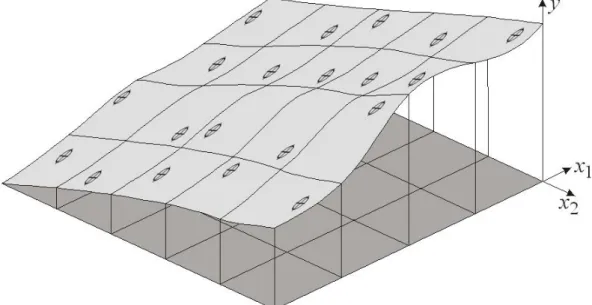
surface, where m of the n inputs are uncertain. As an illustration, Figure 1 shows a response surface for the system y = f(x1, x2), where both x1 and x2 have a range of

values. The output can also be expressed as a PDF of values for y, from which an expectation value and other statistical descriptors can be calculated if required.

Sensitivity is the rate of change of y with respect to a change in an input x. In the simple example illustrated in Figure 1, there are two sensitivities, one with respect to x1, and one with respect to x2. These sensitivities can be evaluated at any point on the

response surface, but in general they are evaluated at the best estimate value for each of the inputs (e.g., at the mean, median or mode of the respective PDFs). If this best estimate or nominal value is designated X0, then the sensitivities are the partial derivatives of output y, with respect to each input at this point:

0 0 ₂ 1 , X X x y x y       ∂ ∂       ∂ ∂ (2)

A disadvantage of this simple measure of sensitivity is that it is dependent on the units of the variables involved. The sensitivity to x1 will be a thousand times greater if the

units are millimetres than if they are metres. This disadvantage can be overcome by normalising the sensitivities and expressing them as relative values:

0 0 2 2 0 0 1 1 0 0 , y x x y y x x y X X ×       ∂ ∂ ×       ∂ ∂ ₍₃₎

These measures of sensitivity take no account of the uncertainties in the input, although a variable with a low sensitivity but large uncertainty may be as important as a variable with a greater sensitivity but smaller uncertainty. The contribution of a variable to the overall uncertainty can be expressed as the product of its sensitivity and standard deviation:

x X x y _×σ     ∂ ∂ 0 (4)

The Gaussian approximation3 can then be used to estimate the uncertainty of the output in terms of its variance:

              ∂ ∂ +               ∂ ∂ ≈ Var[ ] Var[ ] ] Var[ ₂ 2 2 1 2 1 0 0 x x y x x y y X X (5)

where Var[x₁]≡σ2_x1 and Var[x₂]≡σ2_x2.

Each of these measures can be extended to account for larger numbers of inputs. Whatever the number of input parameters involved, however, these measures all remain local measures of uncertainty around the nominal value of the output (y0). To

3 _{The Gaussian approximation states that the variance of the output can be reliably estimated by the}

take account of the behaviour of the full range of the output, it is necessary to use techniques that involve the full range of the input variables.

One approach that takes more account of parameter uncertainty than the above local measures uses a ‘high’ and a ‘low’ value for each parameter. These need not be the extremes of the distribution, but should encompass the central part of the distribution. The “nominal range sensitivity” is then calculated by varying each parameter from its high to low value, while keeping all other parameters at their nominal value. If the low and high values for the two parameters are denoted by [_x1−,_x1+]and[_x2−,_x2+]_{, then} the nominal range sensitivities are:

) , ( ) , ( ) , ( 0 2 1 0 2 1 1 y f x x f x x x U = + − − and (6) ) , ( ) , ( ) , ( 0 ₂ 1 2 0 1 2 y = f x x+ −f x x− x U (7)

Although these measures are more than local, they are less than global because they hold all but one of the parameters constant. In many systems, the effects of varying one input are dependent on the values of other parameters. In these cases, a joint parametric analysis, evaluating y for several values of the other parameters, is useful. The case illustrated above with two parameters and two values requires four evaluations of the output. Increasing the number of values and the number of parameters quickly increases the number of evaluations required using this approach. Relationships within the resulting data can be identified by calculating correlation coefficients between different inputs and the output. However, a visual examination of scatter plots (see Section 4.3.5) is also of value, because there are many ways in which distributions with a low correlation coefficient can nevertheless have a significant relationship. For example, situations where there are thresholds or discontinuities may not be identified without a visual examination of the data (see Figure 2).

The following section describes some of the approaches that can be used to decrease the number of evaluations required for systems that are more complex than the examples presented in this section.

2.3

Probabilistic Approaches

As soon as an assessment requires more information than can be obtained from a single evaluation of the output based on a set of input parameter values, it is appropriate to consider ways in which multiple evaluations can be undertaken effectively. For simple systems, with a small number of inputs, parameter distributions defined using simple functions, no correlations between input parameters, and easy to evaluate relationships, the direct evaluation of all the required output values may be the most effective approach. It may be possible to evaluate parts of such systems analytically. As the complexity increases, with more parameters, correlations, discontinuities and complex interactions, and more complex parameter distributions, each individual evaluation requires more effort. The computational effort required to perform large numbers of evaluations for such systems may become unrealistic. This has led to the development of alternative approaches to evaluating the output values and/or to selecting the combinations of

parameter values at which to undertake the calculations. A number of such approaches are described in this section.

The most familiar approach to evaluating the behaviour of system models for radioactive waste disposal in which uncertainties are expressed in terms of probability distribution functions is the simulation approach. In essence, this approach simply evaluates the output for a subset of all the possible combinations of parameter values. There are alternatives to the simulation approach for propagating uncertainties (Helton, 1993):

• Differential analysis

• Response surface methodology

• Fourier amplitude sensitivity test (FAST)

Although these methods are not currently in use in performance assessments, it is useful to review them briefly and to highlight the reasons why the simulation approach has been preferred.

2.3.1 Simulation

All of the approaches that are used to propagate uncertainty from the uncertainty in the inputs require evaluation of the output for specific sets of input values. In some of the approaches described below, the values selected for evaluation form a regular grid or are otherwise pre-selected. This means that the calculated output values cannot necessarily be used to estimate the properties of the overall output distribution. Instead, they are used to develop an approximation or surrogate form of the output which is then used for uncertainty propagation and sensitivity analysis. The simulation approach does not necessarily have this disadvantage and can provide an estimate of the output distribution directly.

In the simplest form of the simulation approach, values are selected at random from the input distributions. The output values calculated from these randomly selected values then form a random subset of all possible output values. Because the calculated output distribution is effectively a sample drawn at random from the overall distribution, the properties of the calculated distribution can be used to estimate the properties of the overall distribution using standard statistical techniques. There are a number of issues that must be considered in the practical implementation of a simulation approach. These include:

• The definition and use of PDFs to define the input distributions.

• Methods used for sampling.

• Accounting for correlations between input parameters

• Determining how many samples are required. These issues are discussed in more detail in Section 3.

2.3.2 Differential analysis

Differential analysis is a method for approximating the full model using a Taylor series, and then using this series in place of the full model for sensitivity and uncertainty analyses.

The Taylor series is developed at the nominal value X0, and expresses deviations of the output from the nominal value (y – y0) in terms of deviations of the inputs from their nominal value ( 0

i

x

x_i − ). Successive terms of the series include higher order deviations and partial derivatives. The second-order series has the form:

0 0 2 1 0 1 0 1 0 0 _{( )( )} 2 1 ) ( X j i n i j j n j i i X i n i i i x x y x x x x x y x x y y         ∂ ∂ ∂ − − +       ∂ ∂ − = −

∑

∑∑

This can be a good approximation to the model if the deviations ( 0

i

x x_i − ) are relatively small and the function is relatively smooth (i.e., the higher derivatives are small).

The Taylor series can be used for uncertainty propagation, although estimates of the tails of the distribution may not be reliable. As an example, the expectation value for y from a second order series is given by:

0 1 1 2 0 _{Cov[ , ]} 2 1 ) E( X n i n j i j j i _{x x} y x x y y

∑∑

where Cov[xi, xj] is the covariance.

If the inputs are uncorrelated, then this reduces to:

) Var( 2 1 ) E( 1 2 2 0 i n i i x x y y y

∑

and the variance can be estimated by:

) ( ) Var( ) Var( 2_{2 3} 1 2 1 i i n i i i n i i x x y x y x x y y _µ      ∂ ∂       ∂ ∂ +       ∂ ∂ ≈

∑

∑

whereµ₃(x_i)is the third central moment for xi (see Section 4.2).

A key point from these estimates is that the expectation value for the output is not equal to the nominal output (i.e., the output calculated using the nominal values for all inputs), unless the model is linear. In the more usual case of a non-linear model, the expectation value is also a function of the variances and covariances of the inputs. The advantages of differential analysis are that it provides a clear approach to uncertainty analysis, with the variance of the output decomposed to the sum of the contributions from each input. Also, the numerical analyses required are generally

simple. The disadvantages are that the derivation of the series can be complex, particularly as higher order terms are included to achieve a satisfactory approximation to complex functions. It is also a local approach to uncertainty analysis and will not be accurate if the model has discontinuities or large uncertainties.

2.3.3 Response surface methodology

The response surface approach involves fitting an approximate response surface to a moderate number of calculated output values, and then using this approximation for uncertainty propagation and analysis. The technique is of value where the computational resources required for evaluating the full model are very high.

Key steps in using the response surface approach are identifying both the key input parameters and the combinations of values for these parameters that will be used to calculate points on the response surface. Parameters to which the response surface is less sensitive can be set to their best estimate or nominal values. A number of experimental design procedures can be used to generate efficient combinations of values. Factorial designs are based on selecting two or more values for each parameter and then using all possible combinations of these values. For a two-level design (i.e., with a ‘high’ and a ‘low’ value for each parameter) with k parameters, a full factorial design will involve 2k _{combinations, a number that can become very}

large for complex systems. Fractional factorial designs, which use a given fraction (e.g. 1/10) of all possible combinations, are more efficient. Care is required in selecting a design for systems involving non-linearities and interactions between inputs so as not to reduce the number of combinations to such an extent that the response surface is not sufficiently well defined. Monte Carlo methods can also be used to define the combinations used to generate the response surface. The issues that apply to this approach are similar to the issues concerning the use of Monte Carlo methods for directly determining the output distribution (see Section 3).

Once the combinations of parameter values (design points) have been selected, the full model is used to calculate the output values at these points. A response surface is fitted to these output values using techniques such as least squares or spline functions. For relatively simple systems, linear or quadratic models may be adequate. Higher order models can be used either to provide a better fit for relatively simple systems or an adequate fit for more complex systems. Regression coefficients are a useful means of assessing how well the response surface fits the output values, but can be misleading if the number of design points is comparable with the number of degrees of freedom for the response surface. Determining how well the response surface matches output values for additional design points located at the extremes of the system is a useful way of assessing its adequacy.

Once a response surface has been established, it can be used for uncertainty propagation and sensitivity analysis. For a linear response surface of the form:

j n j jx b b y

∑

) E( ) E( 1 0 j n j j x b b y

∑

∑

∑ ∑

More complex relationships can be used to determine these values for more complex response surfaces. The alternative approach is to use Monte Carlo simulation with the equation for the response surface. Even with a quadratic or higher order surface, the computation requirements for this simulation will be low and large numbers of samples can be used, giving a good estimate of the distribution function for the response surface.

Sensitivity studies can be based on the response surface, using either analytical methods to calculate normalised sensitivity measures for each parameter, or graphical examination of the results from simulations.

The disadvantages of the response surface approach are related to the effort required to determine the response surface and to the difficulty in defining a response surface that adequately matches the output from a complex model. Typically, the complexity of the system-level models used in performance assessments for radioactive waste disposal means that the output function is too complex to be easily approximated by a response surface. In particular, response surfaces are difficult to implement satisfactorily where there are discontinuities or thresholds in the model output.

Although not generally used for system-level modelling, a response surface approach has been used in several programmes for sub-system analyses. In the WIPP PA, for example, creep closure of the repository is accounted for in assessment calculations by changing the porosity of the waste disposal area. The SANTOS code uses finite element methods to calculate porosity as a function of gas pressure, and a series of porosity time histories is calculated based on a set of thirteen different gas generation potentials. This modelling results in a three-dimensional response surface representing changes in gas pressure and porosity over the 10,000-year simulation period. In the system calculations, the porosity corresponding to the calculated gas pressure and fluid saturations is interpolated from this response surface.

2.3.4 Fourier amplitude sensitivity test (FAST)

The Fourier amplitude approach to sensitivity and uncertainty analysis is based on a transformation of the multi-dimensional integral over all model inputs to a one-dimensional integral which is easier to evaluate. This transformation is achieved by defining a curve in model space, and a Fourier series representation of this curve is then used to estimate the contribution of each input variable to the variance of the model output.

The general form of the one-dimensional integral used to estimate the expectation value for the general model y= f(X) is:

[

]

y (sin( ), (sin( ), _n(sin( _n ) d 2 1 ) E(

∫

where G1, …, Gn and ϖ₁,K,ω_n are series of functions and integers respectively. The

variance can be similarly estimated:

[

]

∫

The advantages of the FAST approach are that it is global, covering the full range of input distributions, and that a surrogate model is not required. The principal disadvantages are the difficulties in deriving the curve in parameter space, the inability to take account of correlations between inputs, and the lack of information about discontinuities or thresholds in the output.

There are no examples of the use of this approach in performance assessments for waste disposal facilities, and its disadvantages mean that it is unlikely to be used for system analyses. It may, however, have a role in some sub-system analyses.

3

Simulation

3.1

Introduction

Simulation is the most common method used for probabilistic calculations, not only in performance assessments for radioactive waste disposal, but also in other sectors. A principal reason for this is that the concept is easy to understand and does not involve any complex mathematics. There is sometimes resistance to adopting a probabilistic approach because of the perceived difficulties of expressing uncertainty as a probability, but the concept of repeating a deterministic calculation many times with different parameter values is a simple one.

Although simple in principal, the application of the simulation approach to a complex problem comprises several stages and requires a number of decisions to be made. The principal stages are:

• Identification of key parameters and uncertainties

• Identification of correlations between parameters

• Model development (conceptual, mathematical and computational)

• Definition of probability distribution functions (PDFs)

• Sampling

• Calculation, and repetition of the calculation a sufficient number of times

• Presentation and analysis of results

During the development, licensing and operation of a disposal facility, a number of assessments will be undertaken. There will be iterations of these principal stages both within an assessment and between successive assessments. In particular, the analysis of results will help to identify the key parameters and where there would be most benefit in reducing uncertainty in subsequent iterations.

The scope of this report does not include a detailed description of all the stages of an assessment. Instead, it focuses on those aspects that are unique to probabilistic calculations. Model development is not discussed, because in principle the same models can be used for deterministic and probabilistic calculations. In practice, different models may be required, both to reduce the computational burden of running a complex model several hundred times, and also because a model used for probabilistic calculations must be robust over a wider range of conditions than a deterministic model applicable to a single set of conditions.

The key areas discussed in this section are the definition of PDFs, sampling, correlation and convergence. The definition of scenarios to be analysed, and specifically the use of sampling to define these, is also discussed. Section 4 describes the presentation and analysis of results.

3.2

Developing Input PDFs

The aim of probabilistic calculations is to take account of uncertainties. In the complex systems that are assessed in performance assessments, there will be uncertainties about many aspects of the system and system behaviour. Whether all of these uncertainties should be addressed is a strategic decision that is dependent upon the resources available and the purpose of the assessment (the assessment context). An assessment solely for design optimisation may, for example, account explicitly for a different set of uncertainties than an assessment aimed at developing a license application.

Any level of uncertainty in parameter values will have some effect on the overall calculated result, but in practise there will be a restricted set of uncertainties that will dominate the overall level of uncertainty. These key uncertainties may result from large uncertainties in the input values, or from sensitivities in the models that make the overall result sensitive to particular parameters. Where there are both large data uncertainties and significant system sensitivities, the final result may be dominated by a very few parameters.

Significant resources can be expended on developing PDFs if processes such as expert elicitation are required or additional site characterisation or experimental programmes are undertaken. There may be other reasons for undertaking additional data collection, such as confidence-building, but it is sensible to have an understanding of the key sensitivities before undue effort is expended on defining PDFs that do not have a significant effect on the calculated result. Paradoxically, the most appropriate tool for determining sensitivities is a probabilistic calculation. A key issue is therefore how to identify sensitivities prior to undertaking the calculations that would help to identify them.

Model sensitivity is not, however, the only criterion for determining the effort or resources that should be expended on defining parameter PDFs. A risk assessment model may be sensitive to parameters such as radionuclide half-life or inventory, for example, but these are known or well constrained and would not normally be input as a PDF. The issue, therefore, is to identify those parameters to which the model is sensitive and for which there are large uncertainties.

The resolution of this paradox lies in the iterative nature of the assessment process. This means that early assessments can use approximations to define levels of uncertainty without significant resources, and the results from these can be used to identify potentially important parameters. Further studies will then allow a better definition of the uncertainties for these parameters. Later assessments can focus on the key uncertainties, and work programmes to reduce the level of uncertainty can be effectively targeted.

Selecting distribution types

There is a large literature on identifying the most appropriate distribution to use in defining PDFs, and on assessing or optimising the “goodness-of-fit”. In studies where the intention of the simulation is to accurately reproduce conditions for which there

are a large number of observations and measurements, obtaining the closest possible match is appropriate. However, in the case of elicited data, or where there are comparatively few observations to define variability or uncertainty, simple distributions that have the same broad characteristics as the data are likely to be adequate, at least in the initial stages of the assessment process. Simple distributions are intuitive and their form can be described in terms familiar to non-statisticians. Figure 3 shows, for example, how a triangular distribution (defined by maximum, minimum and mode) can be substituted for a normal distribution (defined by mean and standard deviation).

There are three main distribution types used in performance assessment programmes, together with their log-transformed equivalents4:

- Uniform and log-uniform - Triangular and log-triangular - Normal and log-normal

Most assessments also have provision for defining a PDF using data pairs rather than a function. This cumulative or empirical distribution allows any data to be used and is useful in cases such as bi-modal data or sparse data that cannot easily be fitted by a function.

In addition to this basic set of distribution types, other distribution types are used for specific purposes. The Beta distribution has been used or proposed in several assessments. It has the benefit of being extremely flexible (Figure 4), but has the disadvantage of not being intuitively related to the data. The WIPP CCA (Appendix PAR) uses a Delta distribution to sample between different conditions or alternative models. The recent SKB report on developing PDFs (Mishra, 2002) uses the Poisson and Weibull distributions to account for data on canister failures.

SYVAC, the assessment code used for the Canadian performance assessment, also allows parameter values to be determined from an explicit equation and a sampled residual error parameter. For example, sorption coefficients for minerals are calculated from an equation fitted to observational data, multiplied by a random error factor to represent the uncertainty in the fitted equation. The error factor is sampled from a log-normal PDF with geometric mean 1.0, geometric standard deviation 3_{10 ,}

and truncated at 0.1 and 10 (± 3σ).

The effects of changing the type of distribution used to characterise uncertainty can be determined mathematically. Calculating the significance of such effects and whether they would significantly affect calculated doses and risks is more difficult because of the interactions and non-linearities present in models of complex systems.

Defining PDFs

There is an overlap between the task of determining which distribution type to use for a particular PDF and defining the values that describe the distribution (maximum,

4 _{A logarithmic distribution is generally more appropriate for parameters where the difference between}

minimum, etc.). As already noted, initial estimates of the maximum, minimum and mean or best-estimate values for a parameter can be made with significantly less resources than required for a comprehensive data review and/or elicitation exercise to define a PDF. Using such initial estimates, probabilistic calculations can be undertaken and sensitivity studies used to identify those parameters for which detailed studies aimed at better defining uncertainties are justified.

Methods for performing sensitivity studies are described in Section 2.2. In the context of deciding which parameters should be examined in detail, it should be noted that two types of sensitivity may be important. Results may be sensitive to parameters that have a linear relationship with the output but which have a wide variation from minimum to maximum. Results may also be sensitive to parameters where there is a much smaller range of uncertainty but which have a non-linear relationship with the output. In these cases, the key sensitivity will probably be to the selected maximum value (or minimum if the relationship is an inverse one). Parameters that display this type of sensitivity to the exact form of the distribution are particularly important to identify because confidence in the overall result may depend on the justification presented for the selected distribution.

In the initial stages of an assessment, the principal method for defining PDFs comprises a provisional analysis of available information and expert judgement. As discussed in Wilmot and Galson (2000), it is important that these judgements are acknowledged and documented even in the early stages because they may otherwise be “lost” if they are incorporated into the later stages of the assessment. Once key parameters have been selected and more formal methods for defining PDFs are adopted, there are two methods available. The first involves a detailed review of the available data, expert judgement as to the reliability and relevance of this information, and fitting a distribution to the data by varying the characteristics of the distribution. The second approach involves expert elicitation to define the shape of the PDF and then fitting a distribution (Wilmot et al., 2000; Hora and Jensen, 2002). In both cases, empirical distributions can be used if the distribution is complex.

A key concern when eliciting distributions is the phenomenon known as anchoring, whereby experts focus on a narrow range of values and underestimate the uncertainty. Facilitators therefore encourage experts to think carefully about circumstances that may give rise to larger or smaller values than their initial estimates. A similar underestimate of uncertainty can arise if experimental data used to develop PDFs is too restrictive and does not correspond, for example, to a wide enough range of physical and chemical conditions. Underestimating parameter uncertainty by defining PDFs that are too “narrow” will lead to an underestimate of uncertainty in the overall performance measure (dose or risk).

Because there is an acknowledged tendency toward anchoring and underestimating uncertainty, there may be a tendency for analysts to extend the range of PDFs in order to compensate. However, if this is done on an ad hoc basis, rather than being justified by documented information or reasoning, it can contribute to a phenomenon known as risk dilution. This is the paradoxical situation in which an increase in uncertainty about contributing factors, which should lead to caution, leads to a decrease in calculated risk and hence makes the system appear “safer”.

Significant risk dilution arising from an over-estimate of parameter uncertainty could occur, but it requires that the additional uncertainty is applied only to the tail of the distribution that lowers the calculated risk. An increase in the other tail, or a symmetrical increase, could in fact lead to “risk amplification” and over-estimate calculated risks. This could be an issue if it is added to other conservatisms in the analysis and suggested that the risks were above regulatory constraints.

3.3

Sampling Methods

Once the parameters to be sampled have been determined and appropriate PDFs defined, probabilistic simulations can be undertaken. Each simulation corresponds to a deterministic calculation, but with parameter values sampled from PDFs rather than being defined a priori. There are three methods that can be used for sampling from PDFs:

• Monte Carlo or random sampling

• Stratified or Importance Sampling

• Latin Hypercube Sampling (LHS)

3.3.1 Monte Carlo sampling

Although random samples can be generated directly from some types of distribution, the computational algorithms used to generate random (or more correctly, pseudo-random) numbers generally give numbers in the range 0 - 1. These can then be mapped to the complementary distribution function for a particular parameter to yield a random value for that parameter. This method is illustrated in Figure 5.

If sufficient random samples are made, then the resulting distribution of parameter values will approach the sampled PDF. However, the number of samples required to ensure that all regions of the PDF are adequately represented can become large if there are low-probability regions in the distribution. Because these low-probability regions generally correspond with the extreme values (tails) of the distribution, it can be important that they are sampled if the full range of system behaviour is to be explored.

In order to be 99% certain that at least one sample lies above the 95th percentile of a distribution, the number of samples required, N, is such that:

1 - 0.95N > 0.99

which gives a value of 90 samples. To provide the same confidence that at least one sample lies above the 99th percentile, some 459 samples would be required.

As the number of sampled parameters increases, there are two approaches to determining the number of samples required. The first approach is to use the same calculation as above to determine how many samples are required to provide confidence that one or more calculated values exceed the required percentile. On this

basis, and provided that the calculated values are independent, the number of samples required is independent of the number of sampled parameters or their distributions. This independence of the number of samples required from the number of parameters sampled arises because this calculation assesses the distribution of calculated values and not the distributions of sampled values. For example, consider a distribution calculated by multiplying sampled values from two uniform distributions (Figure 6). The 95th percentile of this distribution would correspond to samples lying at the 78th percentiles of the sampled distributions:

(1 - 0.78) * (1 - 0.78) = 0.048

This calculation will vary according to the types of distribution involved and how parameters are used in the calculations. However, in general, as the number of parameters increases, the more likely it becomes that the maximum calculated value will lie above a selected percentile without necessarily sampling the extremes of the parameter distributions. As noted above, this could mean that parts of the distributions that could lead to high consequences are not sampled.

The second approach to determining the required number of samples is based on ensuring that the full range of system behaviour is sampled. Again, the exact number of samples required will depend on the types of distribution and the calculation, but the approach can be illustrated using the same example as above. To provide 99% confidence that a pair of sampled values come from above the 95th percentile of their respective distributions, the number of samples required, N, is such that:

1 - [1 - 0.05 2] N > 0.99

which gives a value of 1840 samples. Extending this calculation to 5 sampled parameters:

1 - [1 - 0.05 5] N > 0.99

shows that some 14.8 million sets of sampled values would be required to provide the same confidence that one set represented the combination of the upper 5% from each sampled distribution.

These illustrative examples of the numbers of random samples required show why methods for determining when sufficient simulations have been run (convergence) may be more effective than an a priori determination of the number of samples required. Convergence is discussed in Section 3.5. More efficient approaches to sampling have also been developed. Some of these are discussed in the following sections.

3.3.2 Stratified or Importance Sampling

The number of samples required to fully explore model space using random sampling is large because there is no assurance that particular parts of this space will be sampled. Importance or stratified sampling overcomes this problem by dividing the model space into regions and then sampling from within each region. Generally, the number of samples corresponds with the number of strata, but the size of the strata

can be uniform (equal probability, Figure 7) or variable (unequal probability, Figure 8). In each case, when the calculated values are used to define an output distribution or determine an expectation value, they are weighted according to the probability of the strata.

Equal strata probabilities (stratified sampling) are generally easier to implement, but may require a large number of strata to ensure that low-probability, high-consequence regions are adequately explored. Using unequal probability strata (importance sampling) ensures that such regions can be selectively sampled without an excessive increase in the number of samples (i.e., fewer samples are taken from the high-probability, low-consequence regions), without compromising the validity of the probabilistic approach.

The disadvantage of either approach to stratified sampling is that it requires knowledge of the model space so that the strata and their probabilities can be defined. This is relatively easy when there are only a few parameters and simple relationships between them. However, as the number of sampled parameters increases and the relationships become more complex, it becomes increasingly difficult to determine the characteristics of the model space and hence to define the strata and their probabilities.

Importance sampling was investigated in the HMIP programme of work prior to Dry Run 3. The methodology used was to run pilot simulations to identify parameters and parameter interactions leading to high dose (those that contribute to 95% of the risk estimate) and also times of maximum risk. Importance sampling functions were then defined by fitting beta or log-beta distributions to the cumulative risk curves at the times of maximum risk. Initial studies defined the distributions manually, but algorithms were later developed to automate the process. Sampling efficiencies5 of more than 100 were demonstrated. However, the level of processing required to generate the importance sampling distributions reduced the overall efficiency.

Later HMIP models used methods for environmental simulation, introducing significant variations in the dose-time curves between simulations. This prevents the definition of a generally applicable importance sampling distribution. In Dry Run 3, an importance sampling case was specified in an attempt to improve convergence of a full climate simulation model. This resulted in improved convergence at the time for which importance sampling was specified, but considerably poorer convergence at other times.

3.3.3 Latin Hypercube Sampling

Latin Hypercube Sampling (LHS) has some of the advantages of both random and stratified sampling, but without the requirement to have a priori knowledge of how the parameter distributions and relationships interact to generate the model space. Instead, LHS divides each parameter range into intervals of equal probability and selects one value from each interval (Figure 9). When there are two or more sampled parameters, sample sets are formed by combining values at random from each

5 _{Sampling efficiency here is the ratio of the number of random samples to the number of importance}

parameter set. This combination is done without replacement so that each selected value is used once only in the analysis.

Values can be selected from each interval by random sampling within that interval. An alternative is to use the median value of each interval. Such Median Latin Hypercube Sampling (MLHS) provides more evenly distributed samples than random LHS. For a parameter that is defined as a single continuous distribution, the PDF generated using MLHS will usually look fairly smooth, even with a small sample size (such as 20), whereas the result using random LHS may look noisy. As sample size increases, the distinction between output from the two approaches becomes less. MLHS requires slightly less computational effort than random LHS, although the effort saved is unlikely to be significant in comparison with the overall computational effort required for an assessment model. MLHS also yields the same set of sampled values each time a distribution is “sampled”, if the number of samples is constant. This may be an advantage when system behaviour is being studied, although the order in which values are combined to form sample sets may lead to differences in the calculated output. MLHS can generate a distribution that is not representative of the true parameter distribution, specifically when the true distribution has a periodic function with a period similar to the size of the equiprobable intervals. However, parameters used in assessment models do not typically vary according to a periodic function of this kind.

The principal advantage of LHS is that it ensures that the entire range of each parameter is sampled, which in turn means that the distribution of sample sets will be more uniformly distributed across model space than with the same number of random samples. Helton and Davis (2001) show that, above a certain sample size, LHS results in calculated outputs with lower variance than those generated by random sampling.

Although it is not necessarily the case that the most important effects associated with a particular parameter only occur at the tails of the distribution, these tails, and the interactions between them, are commonly of interest. This interest arises both because these interactions can help in understanding system behaviour, and also because low-probability, high-consequence combinations can significantly affect the expectation value. With random sampling, there is no guarantee that the tails of the input distributions will be sampled. With LHS, the tails will be sampled but, because the combination of samples into sample sets is random, there is no guarantee that a sample from the tail of one distribution will be combined with a sample from the tail of a second distribution. Statistical assurance that particular parts of model space are represented in the output distribution can only be provided by increasing the number of samples, and thereby increasing the probability that samples from the tails of the distributions are combined.

The number of samples required to give a specified assurance that the maximum value in the output distribution exceeds the 99th or other percentile can be calculated in the same manner as for random sampling. For example, 299 samples of each parameter will give a 95% confidence that at least one value exceeds the 99th percentile of the calculated distribution. This approach was used to justify the selection of 300 samples to demonstrate compliance with the regulatory criterion in 40 CFR §194.55(d) for the WIPP. The number of samples needed to provide

assurance that particular parts of model space are represented can also be calculated in a similar manner as for random sampling. In this respect, LHS is more efficient than random sampling, but large numbers of samples are still required if the sample sets include more than a few parameters.

3.4

Correlation

A criticism that can be levelled at poorly designed probabilistic calculations is that some simulations evaluate conditions that are not physically realistic. This can occur if parameters that are in reality correlated are defined and sampled using independent PDFs. For example, whereas in reality high values of one parameter would be associated with high values of a second parameter, and low values with low values, sampling from independent PDFs could combine high values of one parameter with low values of the other. If such combinations are not physically realistic, then any doses or other end-point calculated as a result will not be meaningful. In some circumstances, such erroneously calculated doses may lie within the central part of the calculated distribution, and therefore have no significant effect on the overall result. In other circumstances, however, unrealistic conditions can lead to calculated doses in the tails of the output distribution and thus significantly affect the calculated expectation value.

A specific element of the modelling methodology used in Her Majesty’s Inspectorate of Pollution’s (HMIP) Dry Run 3 was the re-examination of simulations that contributed significantly to risk. This step was to allow for the elimination of any simulations that modelled conditions that were physically unreasonable. Although a close examination of the results should be a part of the analysis of all assessment calculations, determining whether sampled conditions are realistic or unrealistic is a subjective process. Eliminating high dose cases on the basis of such judgements, and thereby reducing the overall expectation value of dose or risk, may not be transparent and could introduce an unintentional bias to the results. With large numbers of simulations, it is not feasible to apply the same level of scrutiny to all sets of sampled conditions. This means that unrealistic conditions that result in low doses are left in the analysis results, lowering the overall calculated dose or risk. This is another example of how risk dilution can arise if an assessment is poorly planned.

The most appropriate method for reducing the potential for simulations to represent unrealistic conditions is to account for correlations within the definitions of parameters and in the sampling stages of the analysis. Correlations between parameters can be accounted for in assessments in several ways:

• Explicit relationships in the equations of the computational models. This approach means that values for one parameter are calculated from the sampled values for one or more other parameters.

• A sampled parameter is used to select between different PDFs for one or more other parameters (Figure 10).

• A limited number of calculations using detailed models is used to define a response surface relating two or more parameters. This response surface is sampled and the corresponding parameter values used in assessment calculations.

• A normally distributed parameter can be correlated with another normally distributed parameter by adjusting the sampled values by a factor including the correlation coefficient and a normally distributed random number. Groups of parameters can be correlated by use of a dummy parameter.

• A sampling protocol is used to ensure that sampled values for two parameters reproduce the observed correlation between the parameters.

The first of these approaches is prescriptive and does not allow for any uncertainty concerning the extent of the correlation. It may nevertheless be of value where alternatives are not available and where independent sampling could cause significant errors. The second approach is more flexible, but the first parameter is effectively restricted to only a few possible values. For example, the selection of redox conditions by sampling could be used to determine the distributions to be sampled for radionuclide solubility, but only about four sets of redox conditions and associated PDFs for solubility could realistically be established.

The response surface technique is useful under certain specific circumstances. When the relationship between two or more parameters is relatively simple, other approaches are probably more efficient. However, when there are more complex relationships between parameters, which cannot be incorporated into a system model without excessively increasing run-times, a response surface can be calculated using a stand-alone detailed model. Sampling from this allows consistent sets of parameter values to be used in the simplified system model and reduces the potential for generating unrealistic conditions.

The method for generating a correlated parameter using the correlation coefficient and a random number is presented in Box 1, and an example is shown in Figure 11. This is a useful technique but is limited in its application because it is restricted to normally distributed parameters.

The final approach listed above for introducing correlations is the most flexible, in that it can be applied to any type of distribution (and the correlated parameters need not have the same type of distribution), and more than two parameters can be correlated. This approach does, however, require additional steps in the modelling process and has also only been implemented in conjunction with LHS. A full description of the method is given in Iman and Conover (1982) and the mathematics are summarised in Helton and Davis (2001). An outline of the method is presented below.

The implementation of correlation into the LHS process uses the rank correlation coefficient (RCC) between the parameters rather than a correlation coefficient describing the relationship between parameter values. The RCC is determined by ranking the values for each parameter (the smallest value is ranked 1 and the largest is ranked n, where n is the number of observations) and then calculating the correlation between the ranks for each pair of values. The RCC is not only easier to implement in a sampling scheme, but it also allows for different types of parameter distribution to be sampled without changing other aspects of the model.

Table 1 illustrates a small set of observations and the calculated relationships and correlations.

The initial step for incorporating correlation into a LHS scheme is to sample the parameter PDFs. For each parameter, this gives n samples, each representing an equally probable part of the input distribution. Each set of sampled values is then rank ordered, and, instead of randomly selecting pairs of values, the pairs are selected so as to match the RCC. For example, if there was perfect correlation (RCC = 1), then the samples would be paired in rank order (rx1, ry1 ; … ; rxn, ryn), and if there was

a perfect inverse relationship (RCC= -1), then the samples would be paired in reverse order of their ranks (rx1, ryn ; … ; rxn, ry1).

Box 1 - Generating correlated distributions

A normally distributed parameter x with a specified correlation to a normally distributed parameter y can be generated from the relationship:

z C C y x₌µ_X+( ₋µ_Y) σ_X /σ_{Y +} (1₋ 2)σ_X where:

x sampled value of X adjusted for correlation to Y

Y

X µ

µ , specified means for X and Y

Y

X σ

σ , specified standard deviations for X and Y y sampled value of Y

C specified correlation between X and Y

Observations Ranks x y rx ry 1 10 2 1 1 2 15 6 2 4 3 22 4 3 2 4 30 5 4 3 5 45 8 5 5 y = 0.13x + 1.84 Correlation coefficient = 0.8 Rank correlation coefficient = 0.7

Table 1. Calculation of the rank correlation coefficient for a set of observations.

The method for pairing samples at other values of the RCC is based on a target correlation matrix that reflects the required correlation structure between parameters6. The sample matrix cannot be manipulated directly, and instead an independent matrix of scores is manipulated using a factorisation of the desired correlation matrix. The selection of the independent matrix is key to the validity of the approach as it determines how well the correlation of the manipulated matrix matches the desired correlation matrix. The scores used by Iman and Conover (1982) are approximations to Normal scores7. These scores were found to be generally effective and have been incorporated into the computer program developed to implement this approach (Wyss and Jorgenson, 1998).

Having manipulated the independent matrix, and checked that the resulting rank correlation matrix closely matches the target matrix, the sample matrix can then be ordered in the same way so as to give the same RCC.

3.5

Convergence

The model space that represents the interactions between all of the input parameters (and across the full range of these parameters) cannot, in general, be defined analytically. Probabilistic approaches are a means of overcoming this drawback by calculating the value of the output parameter(s) at various points across the model space. The model space for real systems is likely to be complex and not represented by a simple surface (see the discussion in Section 2.3). Conducting only a few

6 _{More than two parameters can be correlated using this approach.}

7 _{Obtained by evaluating the inverse cumulative Normal distribution function (Φ}-1_{) at the values of the}

ranks scaled into the interval (0,1) using the van der Waerden transformation. The score si for

calculations is unlikely to adequately represent this surface, and the expectation value calculated from a few calculations may differ significantly from the expectation value for the model surface. An infinite number of calculations could fully reproduce the model surface and give an exact estimate of the expectation value. This is clearly impractical, and the aim of a well-designed probabilistic analysis is to perform sufficient calculations to provide a reasonable representation of the model surface and estimate of the expectation value.

Two approaches can be taken to determining the number of calculations required. The first relies on general statistical relationships to determine the required number of samples a priori. The second approach is based on repeated examination of the calculated results to determine whether they adequately represent the system or if more calculations are required.

The a priori determination of the number of calculations required is based on the premise that, if samples are drawn at random from the input distributions, then the output distribution can be regarded as a random sample of the output population (model space). However, determining how many samples are required to ensure that this random sample is an adequate representation requires further assumptions about the form of the model surface. Assuming, for example, that a “95% confidence of at least one value being above the 99th percentile”8 is a reasonable measure of adequacy has an implicit assumption about the form of the output. If these implicit assumptions are not met, for example if the distribution is highly skewed, then the number of calculations may not be sufficient to provide a reasonable estimate of the expectation value.

Conceptually, the second approach does not require any assumptions about the form of the model surface. Instead, a comparison is made between the calculated output distribution and the model surface. As more and more calculations are performed, these two distributions will converge. A measure of how similar they are at any stage can be compared to an established criterion and a decision made as to whether more calculations are required.

The drawback of this approach to assessing convergence is that the form of the model surface is unknown, so that a direct comparison cannot be made. Various surrogate measures can be used, but these are based on assumptions about the form of the distributions and some caution is still required in their interpretation. The most common approach is based on the standard error of the mean (SEM).

If a sample set is taken from a population, then the mean of the sample set provides an estimate of the mean of the population. If a number of independent sample sets are taken, then the means will form a distribution. For a large sample, the distribution of the sample means is approximately a normal distribution, even if the population from which the samples were drawn is not a normal distribution. The central limit theorem states that the standard deviation of this distribution (termed the SEM) is equal to the standard deviation of the population divided by the square root of the sample size:

8 _{This is the criterion for determining the number of samples required in the regulations applicable to}