Aerosol parameterizations in space-based near-infrared retrievals of carbon dioxide

DISSERTATION

AEROSOL PARAMETERIZATIONS IN SPACE-BASED NEAR-INFRARED RETRIEVALS OF CARBON DIOXIDE

Submitted by Robert Roland Nelson Department of Atmospheric Science

In partial fulfillment of the requirements For the Degree of Doctor of Philosophy

Colorado State University Fort Collins, Colorado

Spring 2019

Doctoral Committee:

Advisor: Christian D. Kummerow Co-Advisor: Christopher W. O’Dell A. Scott Denning

Jeffrey R. Pierce Jennifer A. Hoeting

Copyright by Robert Roland Nelson 2019 All Rights Reserved

ABSTRACT

AEROSOL PARAMETERIZATIONS IN SPACE-BASED NEAR-INFRARED RETRIEVALS OF CARBON DIOXIDE

The scattering effects of clouds and aerosols are one of the primary sources of error when making space-based measurements of carbon dioxide. This work describes multiple investigations into optimizing how aerosols are parameterized in retrievals of the column-averaged dry-air mole fraction of carbon dioxide (XCO2) performed on near-infrared measurements of reflected sunlight from the Orbiting Carbon Observatory-2 (OCO-2). The primary goal is to enhance both the pre-cision and accuracy of the XCO2 measurements by improving the way aerosols are handled in the NASA Atmospheric CO2 Observations from Space (ACOS) retrieval algorithm. Two studies were performed: one on using better informed aerosol priors in the retrieval and another on re-ducing the complexity of the aerosol parameterization. It was found that using ancillary aerosol information from the Goddard Earth Observing System Model, Version 5 (GEOS-5) resulted in a small improvement against multiple validation sources but that the improvements were restricted by the accuracy and limitations of the model. Implementing simplified aerosol parameterizations that allowed for the retrieval of fewer parameters sometimes resulted in small improvements in XCO2, but further work is needed to determine the optimal way to handle the scattering effects of clouds and aerosols in near-infrared measurements of XCO2. With several multi-million dollar space-based greenhouse gas measurement missions scheduled and in development, the massive amount of measurements will be an incredible boon to the global scientific community, but only if the precision and accuracy of the data are sufficient.

ACKNOWLEDGEMENTS

These six and a half years in Colorado have been an amazing experience for me both academi-cally and professionally. It would not have happened if Chris O’Dell had not been willing to take a chance on someone who did not know the difference between a passive and active instrument. I am forever indebted to Chris for taking me on as his first student and mentoring me through both a master’s and doctoral degree here at Colorado State University (CSU). It was a learning process for the both of us but, in the end, a success.

I would like to thank Dr. Chris Kummerow for acting as my academic advisor for the past few years and for providing advice on how to navigate both graduate school and the professional world. Additionally, I wish to thank Jamie Schmidt, Sarah Tisdale, Holli Knutson, and the entire past and present CSU and Cooperative Institute for Research in the Atmosphere (CIRA) administrative staff for their endless patience and knowledge.

I am extremely grateful to have worked with an outstanding set of individuals during my time here. Thank you to Tommy Taylor for always being available to chat about research and for foster-ing my new cyclfoster-ing addiction, thanks to Andy Manaster and Emily Bell for befoster-ing great officemates, and thanks to Andy Schuh, Heather Cronk, David Baker, Natalie Tourville, Hannakaisa Lindqvist, Michael Cheeseman, and Greg McGarragh for the thoughtful discussions and mentorship. Addi-tionally, my committee has been patient and supportive throughout my graduate program. Thank you Chris O’Dell, Chris Kummerow, Scott Denning, Jeff Pierce, and Jennifer Hoeting.

The OCO-2 team at the NASA Jet Propulsion Laboratory (JPL) has been extremely supportive of my work over the years and I could not have asked for a more friendly, enthusiastic group of scientists to call my co-workers and friends. I thank them all, especially Annmarie Eldering and Dave Crisp, for acting as mentors as I continue to grow as a young scientist.

Finally, I would like to thank my friends and family. My loving girlfriend, Ariel, has supported me this past year as I worked to finish my studies. The number of friends I have made in Colorado

is too large to list here, but thank you all for being a part of my life. I am fortunate to have a mother who, despite us not agreeing on many things, has always been supportive.

TABLE OF CONTENTS

ABSTRACT . . . ii

ACKNOWLEDGEMENTS . . . iii

LIST OF TABLES . . . vii

LIST OF FIGURES . . . viii

Chapter 1 Introduction . . . 1

1.1 Greenhouse Gases and Climate . . . 1

1.2 Understanding Carbon Dioxide Absorption Mechanisms . . . 3

1.3 The Importance of Carbon Dioxide Measurements . . . 6

1.3.1 The Orbiting Carbon Observatory-2 . . . 11

1.3.2 Future Missions . . . 13

1.4 Retrieving Carbon Dioxide from Satellites . . . 15

1.4.1 Optimal Estimation . . . 17

1.5 Cloud and Aerosol Errors in XCO2 Retrievals . . . 20

1.5.1 Scattering Effects of Clouds and Aerosols . . . 21

1.5.2 Screening Methods . . . 22

1.6 Aerosol Parameterizations in Near-Infrared Measurements of GHGs . . . . 24

1.6.1 ACOS Aerosol Parameterization . . . 25

1.7 Outline . . . 26

Chapter 2 The Impact of Improved Aerosol Priors on Near-Infrared Measurements of Carbon Dioxide . . . 29

2.1 ACOS Aerosol Parameterization . . . 29

2.2 Validation Datasets . . . 30

2.2.1 TCCON and AERONET Validation Dataset . . . 30

2.2.2 Model Validation Dataset . . . 32

2.3 Filtering and Bias Correction . . . 32

2.4 Modeled Aerosol Priors . . . 34

2.4.1 Types and Optical Depths . . . 37

2.4.2 Types and Gaussian Fits . . . 37

2.4.3 Types and Scale Factors . . . 37

2.4.4 Aerosol Prior Uncertainties . . . 39

2.5 Results . . . 42

2.5.1 TCCON Validation Results . . . 42

2.5.2 Model Validation Results . . . 44

2.6 Conclusions . . . 54

Chapter 3 Simplified Aerosol Parameterizations in Near-Infrared Retrievals of Carbon Dioxide . . . 57

3.1 Simplified Aerosol Parameterizations . . . 57

3.2.1 Synthetic Dataset . . . 61

3.2.2 TCCON Validation Dataset . . . 63

3.3 Synthetic OCO-2 Observation Results . . . 64

3.4 OCO-2 Observation Results . . . 70

3.4.1 Non-Scattering Retrieval . . . 71

3.4.2 One Layer Model . . . 71

3.4.3 Two Layer Model . . . 72

3.5 Retrieving Aerosol Properties . . . 74

3.6 Conclusions . . . 75

Chapter 4 Conclusions and Discussion . . . 78

4.1 Summary of Results . . . 78

4.2 The Future of Space-Based Measurements of CO2 . . . 80

Bibliography . . . 82

Appendix A High-Accuracy Measurements of Total Column Water Vapor from the Orbit-ing Carbon Observatory-2 . . . 107

A.1 The Importance of Water Vapor . . . 107

A.2 Theoretical Basis . . . 108

A.3 Data . . . 113

A.4 Validation . . . 118

LIST OF TABLES

1.1 Spectral Band Properties . . . 16

1.2 ACOS B8 State Vector Elements . . . 19

2.1 TCCON Site Details . . . 31

2.2 Aerosol Prior Uncertainties . . . 41

3.1 Simplified Aerosol Parameterization Setups . . . 61

3.2 Synthetic OCO-2 Observation Setup . . . 62

A.1 OCO-2 Prior TCWV Validation: Simulations . . . 112

A.2 OCO-2 Retrieved TCWV Validation: Simulations . . . 112

A.3 OCO-2 TCWV Validation Statistics . . . 117

A.4 ECMWF TCWV Validation Statistics . . . 121

LIST OF FIGURES

1.1 Global Average Surface Temperature Change . . . 2

1.2 Carbon Budget Diagram . . . 4

1.3 Uncertainty Reduction from GOSAT . . . 5

1.4 WMO GAW Network . . . 7

1.5 Rayner and O’Brien XCO2 Uncertainty . . . 8

1.6 GOSAT XCO2 . . . 10

1.7 OCO-2 Footprints and Radiances . . . 12

1.8 OCO-2 Observation Modes . . . 13

1.9 GHG Satellite Timeline . . . 14

1.10 Light Path Conceptual Diagram . . . 15

1.11 Measured Radiances . . . 16

1.12 Non-Scattering XCO2 Retrieval Errors . . . 21

1.13 OCO-2 and MODIS Cloud Screening Agreement . . . 24

1.14 ACOS B8 Prior Aerosol Profiles . . . 27

2.1 TCCON and AERONET site map . . . 31

2.2 AERONET AOD Comparisons . . . 35

2.3 MERRA-2 and GEOS-5 Primary Aerosol Type Map . . . 36

2.4 GEOS-5 Aerosol Gaussians . . . 38

2.5 GEOS-5 Aerosol Prior TCCON Results . . . 43

2.6 GEOS-5 Types and AODs with Low Uncertainty Model Comparison Results . . . 45

2.7 GEOS-5 Types and AODs with Low Uncertainty Model Comparison Results, Differ-ence Maps . . . 46

2.8 MERRA-2 and GEOS-5 Prior AOD Maps . . . 49

2.9 MERRA-2 and GEOS-5 Retrieved AOD Maps . . . 51

2.10 GEOS-5 Aerosol Type Test Map . . . 52

2.11 Retrieved Stratospheric Aerosol Impact on XCO2 . . . 53

2.12 Prior AOD Uncertainty Impact on XCO2 . . . 55

3.1 Frankenberg Aerosol Averaging Kernels . . . 58

3.2 Two Layer Model Diagram . . . 60

3.3 Simplified Aerosol Parameterization Synthetic XCO2 Results . . . 65

3.4 Simplified Aerosol Parameterization Synthetic XCO2 Results, Sulfate Only . . . 68

3.5 Simplified Aerosol Parameterization Synthetic XCO2 Results, Iterations . . . 69

3.6 Simplified Aerosol Parameterization XCO2 Compared to TCCON . . . 70

3.7 Two Layer Model Difference Maps Against Model Validation . . . 73

3.8 Effective Radius Retrieval Results . . . 75

A.1 OCO-2 H2O Spectra . . . 109

A.2 Simulated OCO-2 Prior and Retrieved TCWV Heatmaps . . . 111

A.5 OCO-2 TCWV Validation Heatmap . . . 119

A.6 ECMWF TCWV Validation Heatmap . . . 120

A.7 MERRA-2 TCWV Validation Heatmap . . . 122

A.8 TCWV Validation RMSDs . . . 123

Chapter 1

Introduction

1.1

Greenhouse Gases and Climate

The radiative balance of Earth is governed by a number of factors. One such factor is the composition of the atmosphere. Despite representing a relatively small fraction of the total number of molecules in the air, gases such as carbon dioxide (CO2) and methane (CH4) have the ability to trap a substantial amount of heat [1, 2]. This results in Earth being warmer than if there were no atmosphere at all, which has been likened to a “greenhouse effect."

Since the industrial revolution, humans have directly contributed to a substantial rise in the concentration of greenhouse gases (GHGs) in Earth’s atmosphere [2]. This, in turn, has resulted in an imbalance in the radiative budget of Earth, the direct consequence of which is rising global tem-peratures. The atmospheric concentration of CO2has increased by around 46% from pre-industrial times to 2017, from 280 parts per million (ppm) to around 405 ppm, with humans emitting about 37 billion tons of CO2 to the atmosphere each year [3]. This has happened primarily because of the burning of fossil fuels, biomass burning, cement production, and land use change. As of 2011, anthropogenic CO2 represents 1.82 Wm−2 of radiative forcing [2]. However, this forcing and the year-to-year CO2 concentrations are not constant and the mechanisms behind what drives this variability are not fully understood.

Our current trajectory is likely to result in an increase in natural disasters such as heat waves, droughts, and floods [2]. There have been a number of attempts by the global community to try and limit future emissions, including the Kyoto Protocol, Copenhagen Accord, and more recently the Paris Agreement. However, how humans will act in the future is difficult to predict. This means there is considerable uncertainty surrounding the future of Earth’s climate and the world must be prepared for a wide range of potential scenarios. Figure 1.1 shows future warming predictions,

based on the Intergovernmental Panel on Climate Change (IPCC) Representative Concentration Pathways (RCPs).

Figure 1.1: Coupled Model Intercomparison Project Phase 5 (CMIP5) multi-model simulated time series from 1950 to 2100 for the change in global annual mean surface temperature relative to 1986-2005. Time series of projections and a measure of uncertainty (shading) are shown for scenarios RCP2.6 (blue) and RCP8.5 (red). Black (grey shading) is the modeled historical evolution using historical reconstructed forc-ings. The mean and associated uncertainties averaged over 2081-2100 are given for all RCP scenarios as colored vertical bars. The numbers of CMIP5 models used to calculate the multi-model mean is indicated. Taken from [2].

In an attempt to limit GHG emissions, the United Nations Framework Convention on Climate Change (UNFCCC) was created in 1994. The first major effort to address global emissions was the UNFCCC’s Kyoto Protocol, adopted in 1997. This committed numerous countries to limit their emissions to “a level that would prevent dangerous anthropogenic interference with the cli-mate system." However, one of the largest emitters, the United States of America, did not ratify the Protocol. Since then, there has been an amendment (the Doha Amendment) to extend those commitments that has been signed by a fraction of the original countries. At the 21st session of the Conference of the Parties (COP21) of the UNFCCC in 2015, the Paris Agreement was im-plemented in order to limit the increase in globally averaged temperatures to less than 2 degrees Celsius (◦C) above pre-industrial levels. Each party at COP21, representing more than 200 coun-tries, defined and submitted their own nationally determined contribution (NDC) and agreed to

report their GHG emissions to the UNFCCC. These NDCs represent each party’s emission reduc-tion goals and contribureduc-tions to the global effort to stay under 2◦C.

1.2

Understanding Carbon Dioxide Absorption Mechanisms

Carbon dioxide measurements represent one of the primary sources of information that the scientific community has at its disposal to study the current state of Earth’s atmosphere as well as predict potential climate scenarios. CO2 measurements are fed into carbon transport inversion models, which are used to track the gas as it is transported around the atmosphere and subsequently estimate carbon sources and sinks and their associated uncertainty. That is, where CO2 is emitted and absorbed on the surface of the earth, as CO2 does not have sources or sinks in the atmosphere itself. The natural carbon cycle is driven primarily by photosynthesis and respiration by plants [4] and the solubility of CO2in the ocean [5]. The magnitude of these natural processes is much larger than that of the anthropogenically emitted CO2 but on average the natural sources emit about the same as the natural sinks, creating a balance. Although many of the processes that govern the lifecycle of CO2 are known, the exact locations, magnitudes, and mechanisms behind these sources and sinks remains unknown. About half of the anthropogenically emitted CO2 remains in the atmosphere. The other half is absorbed by net carbon sinks. Figure 1.2 shows that for 2007-2016 it is estimated that 10.7 gigatons of carbon (GtC, where one GtC is equivalent to 3.67 gigatons of CO2) per year are emitted into the atmosphere from fossil fuel burning, industry, and land-use change. About 4.7 GtC yr−1 _{of this stays in the atmosphere, while the land sink absorbs} around 3.0 GtC yr−1 _{and the ocean sink absorbs 2.4 GtC yr}−1_.

The partition between oceanic and terrestrial sinks is uncertain and can vary significantly from year to year. Carbon sources and sinks on land, specifically, likely vary more than the oceanic sink and thus have an even higher degree of uncertainty associated with them [7]. Several factors influence the atmosphere-land CO2exchange including CO2 fertilization, changes in nitrogen de-position, forest regrowth, deforestation, and changes in forest management. Currently, it is thought that the European and North American carbon sinks are the result of forest regrowth in abandoned

Figure 1.2:Carbon budget for 2007-2016. Fluxes are given in GtC yr−1 _{with 1-sigma uncertainties. Taken}

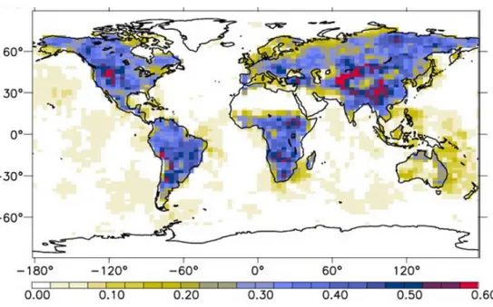
lands, a decrease in forest harvest, boreal warming, and CO2and NO2fertilization. There is some evidence that the tropics are influenced by CO2 fertilization as well [2]. However, there remains considerable uncertainty in estimates of the current flux patterns and, importantly, the exact mech-anisms behind these sources and sinks and how they will act in the future. CO2 measurements help reduce the uncertainty surrounding these sources and sinks because carbon transport inversion models become more accurate when they ingest accurate and precise CO2 measurements [8–11]. Space-based measurements, specifically, provide vastly more global coverage than the currently available network of ground-based measurements. Figure 1.3 demonstrates the expected reduc-tion in uncertainty for eight-day-mean CO2surface fluxes when space-based measurements of the column-averaged dry-air mole fraction of carbon dioxide (XCO2) from the Japanese Greenhouse gas Observing SATellite (GOSAT; [12]) measurements are ingested.

Figure 1.3:Expected uncertainty reduction provided by GOSAT for the estimation of eight-day-mean CO2

surface fluxes. Values are (1 - σa/σb) where σais the posterior error standard deviation and σb is the prior

error standard deviation. Taken from [11].

In addition to answering questions about the fundamental processes that govern the global carbon cycle, space-based CO2 measurements have the potential to improve anthropogenic GHG

emission estimates. Emission reduction goals are traditionally based on “bottom-up" inventories, created by aggregating data from a multitude of sectors and industries that impact the carbon bud-get for a given nation. Current global inventories include the Emission Database for Global Atmo-spheric Research (EDGAR; [13]), Carbon Dioxide Information Analysis Centre (CDIAC; [14]), and the Open-source Data Inventory for Anthropogenic CO2 (ODIAC; [15, 16]). However, these inventories contain considerable uncertainty. Global estimates are thought to be accurate to within 6-10%, but for individual countries, especially in the developing world, those uncertainties can be much larger as they lack the resources to adequately track emissions [17]. Additionally, emis-sions from the developing world represent an ever-growing fraction of the total global emisemis-sions. A potentially more accurate way to constrain these estimates is by creating “top-down" emission estimates. That is, estimates from direct measurements of atmospheric CO2.

1.3

The Importance of Carbon Dioxide Measurements

While well-calibrated ground-based networks of GHG measurements exist, including about 145 stations organized by the World Meteorological Organization (WMO) Global Atmospheric Watch (GAW) [18], they are insufficient when it comes to spatial resolution for CO2and CH4. As shown in Figure 1.4, coverage is lacking in scientifically important regions including the tropics, much of the global oceans, much of Africa, and arctic and boreal regions. Additionally, they lack the coverage to identify or quantify emissions on national scales in order to produce top-down GHG inventories or to provide information about regional scale natural sources and sinks of CO2 [19].

Satellites GHG measurements, however, have the potential to complement the existing in situ network. While there are technical limitations with space-based instruments, their measurements are not beholden to geographic or political boundaries and thus represent a significant improvement over in situ data in terms of global coverage. In order for space-based measurements to be of use to the scientific community, precision and accuracy requirements must be defined and subsequently met. Scientifically, high precision is necessary because even the largest CO2 sources and sinks only produce small changes in the column CO2.

Figure 1.4: The GAW global network for CO2in the last decade. Taken from [18].

Early estimates of the required CO2precision demanded a monthly averaged column precision of better than 2.5 ppm for an 8◦ by 10◦ footprint in order for satellite measurements to be of more use to carbon transport inversion models than just having ground-based in situ measurements [8]. Figure 1.5 shows that the theoretical decrease in uncertainty in CO2 fluxes is reduced as the precision of the XCO2 measurements is improved.

More recent studies have estimated that an accuracy of better than about 0.5% (∼2 ppm for CO2) is required for space-based measurements to be of use in estimating regional carbon fluxes [9, 20–24]. In terms of precision, even a bias of a few tenths of a ppm can be detrimental to carbon transport inversion models [9, 10, 25]. For example, [10] showed that a few tenths of a ppm bias in XCO2 on a regional scale introduced a carbon flux error of over 0.7 GtC yr

−1 _{over temperate} Eurasia. Retrievals of XCO2 are constantly improving and are beginning to approach the level of precision and accuracy needed to study regional sources and sinks [26–31], individual power plants [32], cities [33], etc. However, current single measurement random errors of 0.4 to 1.2 ppm and systematic biases between 1 to 2 ppm still exist over much of the globe [34–36]. Thus, further work is needed to maximize the quality of these data in order for current and future missions to be able to properly answer questions about the carbon cycle.

Figure 1.5: Plot of uncertainty in GtC yr−1against the precision (in ppm) of column-integrated data. The dotted horizontal line shows the prior uncertainty while the dash-dot horizontal line shows the case for the in situ surface network. Taken from [8].

The first space-based instrument to be able to detect CO2 from space was the High-Resolution Infrared Radiation Sounder (HIRS-2; [37]) onboard the Television and Infrared Operational Satel-lite Next Generation (TIROS-N) Operational Vertical Sounder (TOVS; [38]), launched in 1978. However, the estimated accuracy on these thermal infrared measurements was around 10 ppm, which is about the same magnitude as the entire natural seasonal cycle of CO2 [39].

The first dedicated instrument to measure CO2from space was the SCanning Imaging Absorp-tion SpectroMeter for Atmospheric CHartographY (SCIAMACHY, [40]). It was launched by the European Space Agency (ESA) in March of 2002 on board the Environmental Satellite (ENVISAT) and functioned until May of 2012, when communication with ENVISAT was lost. SCIAMACHY had a 30 by 60 km2_{footprint and measured in eight spectral bands, spanning from the ultraviolet to} the shortwave infrared. SCIAMACHY made observations that resulted in continental and seasonal scale variations of CO2 to be observed for the first time [41, 42].

The first mission whose primary objective was to measure GHGs was the Greenhouse gas Observing SATellite (GOSAT), launched on 23 January 2009 by the Japan Aerospace Explo-ration Agency (JAXA), National Institute of Environmental Science (NIES), and the Ministry of the Environment (MOE) of Japan. It contains the Thermal and Near Infrared Sensor for Car-bon Observation-Fourier Transform Spectrometer (TANSO-FTS), which allows for near-infrared measurements of CO2 and CH4, among other things. Near-infrared measurements have a nearly uniform sensitivity to CO2, from the surface up to the middle troposphere. This allows for the column average of CO2 to be estimated. GOSAT also contains the Cloud and Aerosol Imager (TANSO-CAI) for use in cloud and aerosol screening. GOSAT represents a substantial improve-ment in footprint resolution over SCIAMACHY, with an approximate footprint size of 10.5 km. Figure 1.6 shows some of the early XCO2 results from GOSAT.

While NASA had originally planned to launch their own GHG measuring satellite in February of 2009, known as the Orbiting Carbon Observatory (OCO), the launch failed. It took until 2 July 2014 before the spare instrument, named the Orbiting Carbon Observatory-2 (OCO-2), was launched into orbit at the head of the NASA Afternoon Train [43]. OCO-2 represents a further

Figure 1.6:The global distribution of XCO2 for 20-28 April 2009 from GOSAT TANSO-FTS spectra with

signal-to-noise greater than 100 and for cloud-free scenes over land. Taken from [12].

improvement in near-infrared footprint resolution, coming in at approximately 1.29 km by 2.25 km with eight footprints contained along a 10 km swath. Further details about OCO-2, the primary mission studied in this work, can be found in Section 1.3.1.

In December of 2016, the China Meteorological Administration (CMA), Ministry of Sci-ence and Technology of China (MOST), and the Chinese Academy of SciSci-ences (CAS) launched TanSat [44], which contains the Atmospheric Carbon-dioxide Grating Spectrometer (ACGS) and Cloud and Aerosol Polarization Imager (CAPI). TanSat has similar geometric properties to OCO-2, including an 18 km swath containing nine footprints with 2 km by 3 km resolution. Chinese agencies have also launched the Feng-Yun 3D (FY-3D) Greenhouse gases Absorption Spectrome-ter (GAS) and the GaoFen-5 (GF-5) Greenhouse-gases Monitoring Instrument (GMI) satellites in November 2017 and May 2018, respectively. Little published information is currently available on these two missions.

Besides the current suite of near-infrared measurements of GHGs, thermal infrared instruments can also measure CO2, but only in certain parts of the atmosphere as they are not typically

sen-sitive to near the surface. This vertical weighting means that these measurements are unable to resolve surface fluxes and are thus of less use to carbon transport inversion models. Besides HIRS, discussed above, these instruments include the Atmospheric Infrared Sounder [45], the Infrared At-mospheric Sounding Interferometer [46], and the Tropospheric Emission Spectrometer [47]. Solar occultation measurements have also been taken by SCIAMACHY as well as a Fourier Transform Spectrometer (FTS) onboard the Atmospheric Chemistry Experiment (ACE) on SciSat [48]. These measurements produce profiles of GHGs, but the lack of measurements below approximately 5 km due to viewing and geometric restrictions again precludes them from studying surface carbon fluxes.

1.3.1

The Orbiting Carbon Observatory-2

OCO-2 is in a 98.8 minute sun synchronous orbit with a 13:36 local time equatorial cross-ing time for its ascendcross-ing node. OCO-2 measures near-infrared reflected sunlight in three high-resolution spectral bands using a three-channel imaging grating spectrometer and, like other near-infrared instruments, is sensitive to the whole column of CO2. It has a repeat cycle of typically 16 days, but because of the narrow footprint (eight adjacent footprints of 1.29 km by 2.25 km), does not actually measure much of the earth. OCO-2 is also unique in that its primary mission is only to measure CO2. Along with GOSAT, OCO-2 is restricted to daytime measurements of near-infrared reflected sunlight. Figure 1.7 shows an example of the eight OCO-2 footprints and corresponding radiances, taken from the OCO-2 Algorithm Theoretical Basis Document (OCO-2 ATBD; [49]).

OCO-2 takes measurements in three primary modes: nadir, glint, and target. Nadir mode is when the satellite points directly down to make measurements below the satellite. This mode is effective over land, where the surface bidirectional reflectance distribution functions (BRDFs) allow for incoming sunlight to be scattered in a semi-lambertian manner and thus sufficient light is typically reflected straight upwards, regardless of sun angle. Glint mode, designed for use over ocean, follows the “glint spot" of sunlight reflected off of the liquid water surface. The reflectance of sunlight over water is primarily a function of wind speed and is well-characterized [50]. Target

Figure 1.7: Spatial layout of 8 cross-track footprints for nadir observations over Washington, D.C. Taken from the OCO-2 ATBD [49].

mode is where OCO-2 dithers back and forth over a small target spot on the surface. This is used primarily to target Total Carbon Column Observing Network (TCCON; [51]) stations for use as validation. Figure 1.8 shows the setup of nadir, glint, and target mode observations. Full details of the instrument can be found in the OCO-2 ATBD.

Figure 1.8:Schematic of the OCO-2 observation modes: nadir (a), glint (b), and target (c). Taken from the OCO-2 ATBD [49].

1.3.2

Future Missions

GOSAT-2 was launched on 29 October 2018 and carries TANSO-FTS-2 and TANSO-CAI-2. Both instruments have improved specifications compared to the original GOSAT mission including additional bands and an intelligent pointing algorithm. In March of 2019 the instrument backup to OCO-2 will be launched as the Orbiting Carbon Observatory-3 (OCO-3) to the International Space Station (ISS) [52]. It will have a different pointing system than OCO-2 which will allow for new opportunities to map large target areas including cities, forests, and coastlines. The ISS’s low inclination orbit will also allow OCO-3 to make measurements of the same location at different times of the day, allowing for investigations into the daily variability of CO2. Being on the ISS will also allow for the use of co-located measurements from other instruments on the platform, including the NASA Global Ecosystem Dynamics Investigation (GEDI, successfully launched on

5 December 2018), the NASA Ecosystem Spaceborne Thermal Radiometer Experiment on Space Station (ECOSTRESS), and the JAXA Hyperspectral Imager Suite (HISUI).

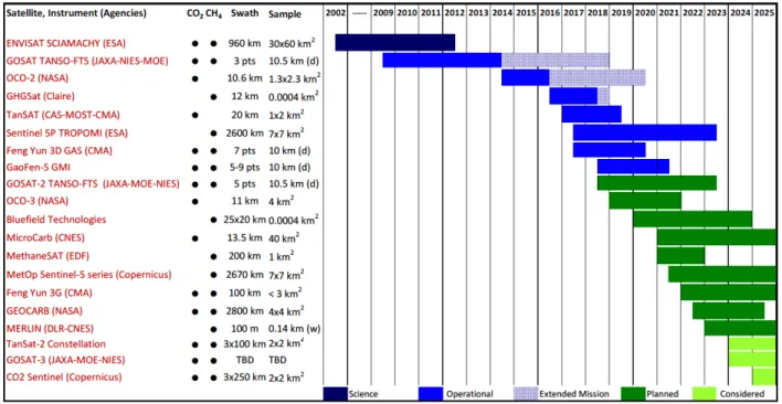
There are several CO2 measuring satellites planned for the years 2019-2023, including Mi-croCarb, GeoCarb [53, 54], Feng-Yun 3G, and GOSAT-3. MicroCarb is being developed by the Centre National d’Etudes Spatiales (CNES) of France. It is similar to other near-infrared sensors but will have an additional oxygen absorption band for better aerosol detection. NASA’s GeoCarb will be the first satellite dedicated to measuring GHGs from geostationary orbit. This will allow for imaging of the Americas potentially multiple times a day. Little is known about Feng-Yun 3G, but it is supposed to be a broad-swath (100 km) imaging grating spectrometer. GOSAT-3 will be an upgraded version of GOSAT-2, with enhanced precision and additional channels. Figure 1.9 shows a timeline of the past, current, and future missions for both CO2and CH4.

Figure 1.9:Timeline of space-based greenhouse gas measurement satellites.

The current and planned space-based GHG missions will be an incredible boon to the scientific community, but only if the data are precise and accurate. The number of global measurements will soon no longer be the limiting factor, but rather the quality of the data itself.

1.4

Retrieving Carbon Dioxide from Satellites

As discussed in Section 1.3, one of the primary ways to measure CO2 concentrations from space is by detecting sunlight that has been reflected off the earth’s surface with hyper-spectral resolution instruments. The number of CO2 molecules in the column of air seen by the instrument, or the “light path", is then estimated and eventually converted to a column-average CO2. This method is conceptually shown in Figure 1.10.

Figure 1.10: The light path is conceptually shown as the yellow beam emitting from the sun, getting re-flected off the surface of the Earth, and being detected by the satellite.

OCO-2 makes use of this method using its three-channel imaging grating spectrometer. The three channels are: a band centered on an oxygen absorption feature at 0.76 µm (the O2 A-band), a relatively weak CO2absorption band located in the near-infrared around 1.61 µm (the weak CO2 band), and a stronger CO2 absorption band in the near-infrared at 2.06 µm (the strong CO2 band). These three bands are used in conjunction to deduce the average amount of CO2 in the column of air seen by the instrument’s sensors. The single value of CO2 in the column of air is specifically known as the column-averaged dry-air mole fraction of carbon dioxide, or XCO2:

XCO2 = R∞ 0 NCO2(z)dz R∞ 0 Nd(z)dz (1.1)

where NCO2(z) is the molecular number density of CO2with respect to dry air at altitude z and Nd(z) is the molecular number density of dry air at altitude z. Because the fraction of oxygen in air is well known (0.20935 parts per part) and near uniform globally, Equation 1.1 can be simplified to: XCO2 = 0.20935 R∞ 0 NCO2(z)dz R∞ 0 NO2(z)dz (1.2)

where the number density of O2 and CO2 can be estimated using measurements of reflected sunlight in the O2 A-band, weak CO2 band, and strong CO2 band. An example of the measured spectra of all three near-infrared bands from OCO-2 is shown in Figure 1.11.

Figure 1.11: An example of measured radiances from OCO-2 in the O2 A-band (left), weak CO2 band

(center), and strong CO2band (right). Taken from [55].

The properties of the three near-infrared bands for OCO-2 are given in Table 1.1.

Table 1.1:Properties of the three near-infrared bands used by OCO-2 to retrieve XCO2. Band Spectral Range Spectral Range # Channels Resolving Power

(cm−1_{) (µm) (λ/δλ)}

O2A 12950-13190 0.758-0.772 1016 >17,000

Weak CO2 6166-6286 1.594-1.619 1016 >20,000 Strong CO2 4810-4897 2.042-2.082 1016 >20,000

The XCO2 retrieval algorithm used in this study was the NASA Atmospheric CO2Observations from Space (ACOS) algorithm (see [56] and [49] for details). It is currently on build 9 (B9), but the majority of this work was done using the previous version (B8). The differences between B8 and B9 were minor and only impacted a small number of retrievals. B10 is currently in development, with an expected public release in spring of 2020.

1.4.1

Optimal Estimation

The ACOS algorithm employs optimal estimation to retrieve XCO2 [57]. This method is useful for combining observations and prior knowledge about a given measurement (“a priori" informa-tion). In near-infrared measurements of GHGs, the detected radiances alone are insufficient to properly constrain all the parameters that impact the estimated variables of interest. This is known as an “under-constrained" problem. Thus, prior information about a given measurement is em-ployed to help guide the estimates. Complete details of the algorithm can be found in the OCO-2 ATBD [49]. Optimal estimation of XCO2 uses a set of variables, or a “state vector", to create a modeled set of radiances, described in Section 1.4, that match the radiances measured by the satel-lite, moderated by prior knowledge of the different state vector elements. This is done by using the state vector parameters found in the forward model, F:

y= F(x, b) + ǫ (1.3)

where y is a vector of the simulated radiances, F is the forward model, x is the state vector, b is a set of other fixed input parameters, and ǫ is instrument and forward model errors. The OCO-2 forward model is designed to simulate radiances using a solar model, radiative transfer (RT) model, and instrument model [49, 58, 59].

The state vector elements are listed in Table 1.2. The parameters selected for inclusion in the state vector typically represent physical quantities to which the measured spectra are sensitive. The exact parameters included in the current ACOS state vector have been refined over the past several years and details on many of them can be found in [56] and [49], with various updates

contained in [60]. Of note, a CO2 profile of 20 layers is retrieved by the algorithm and then used to calculate the total XCO2. Other retrieval algorithms use their own unique covariance matrices and CO2 profile parameterizations, discussed in Section 1.6. Aerosols, surface characteristics, and Empirical Orthogonal Functions (EOFs), etc. are all included in the state vector to allow the retrieval to optimally fit the measured radiances. Certain parameters that impact the measured radiances are not retrieved, either because their impact is negligible, e.g. ozone absorption, or the impact is very well characterized, e.g. Rayleigh scattering.

The simulated radiances, y, are used in an inverse model to try and minimize the χ2 _cost function given by:

χ2 = (F(x) − y)TS−1_ǫ (F(x) − y) + (x − xa)TS−1a (x − xa) (1.4)

where Sǫis the observation error covariance matrix, xais the a priori state vector, and Sais the

a priorierror covariance matrix. The a priori state vector and its corresponding error covariance

matrix are derived from several sources including the Goddard Earth Observing System Model, Version 5 Forward Processing for Instrument Teams (GEOS-5 FP-IT; [62]) for the meteorological variables and zonally averaged seasonal cycles coupled with a typical atmospheric growth rate for CO2. In optimal estimation, the prior and posterior errors are assumed to be Gaussian. The expected value, ˆx, is given by:

ˆ x= xa+ (KTS−1y K+ S −1 a ) −1 KTS−1_y (y − Kxa) (1.5)

where Sy is the a posteriori error covariance matrix and K is the Jacobian, which is the partial derivative of the radiance spectrum for each state vector element:

Kij =

∂Fi(x) ∂xj

(1.6)

The Levenberg-Marquardt modification of the Gauss-Newton method [57] is then used to iter-atively minimize the cost function described by 1.4:

Table 1.2: State vector elements of the ACOS XCO2 retrieval algorithm, adapted from [60]. Name Quantities A PrioriValue A Priori1σ Error Notes

CO2 20 TCCON [56] On sigma

pressure levels1

Temperature Offset 1 0 K 5 K Offset to

prior profile

Surface Pressure 1 GEOS-5 FP-IT 4 hPa

H2O Scale Factor 1 1.0 0.5 Multiplier on

prior profile Aerosol Type 1,2 OD2 _{2 MERRA-2}3 _{±factor of 7.39}

Water, Ice Cloud OD2 _{2 0.0125 ±factor of 6.05}

Aerosol Type 1,2 Height4 _{2 0.9 0.2}

Water Cloud Height4 _{1 0.75 0.4}

Ice Cloud Height4 _{1 Tropopause}5 _0.2

Aerosol Type 1,2 Width 2 0.05 0.01

Water Cloud Width 1 0.1 0.01

Ice Cloud Width 1 0.04 0.01

UTLS Aerosol OD2 _{1 0.006 ±factor of 6.05}

Albedo Mean Land 1/band Prior Calc. 1.0

Albedo Slope Land 1/band 0.0 0.0005

Albedo Mean Ocean 1/band 0.02 {0.2,0.2,1e-3}

Albedo Slope Ocean 1/band 0.0 1.0

SIF Mean6 _{1 Prior Calc. 0.008 Land only}

SIF Slope 1 0.0018 0.0007 Land only

Wind Speed 1 GEOS-5 FP-IT 5 m/s Ocean only

Dispersion Shift 1/band 0.0 0.4 of channel FWHM

Dispersion Stretch 1/band 0.0 1 pm/channel

EOF Amplitudes 3/band 0.0 10.0

1 _CO

2profile contain 20 or fewer elements, depending on the surface pressure.

2 _{Optical Depth at 0.76 µm.} 3 _{Monthly climatology from 2006.}

4 _{Peak heights of the Gaussian distributions.} 5 _{Estimate from GEOS-5 FP-IT parameters.} 6 _{See [61].}

xi+1= xi+ (KTiSǫ−1Ki+ (1 + γ)S−1a ) −1

[KTi S −1

ǫ (y − F(xi)) + S−1a (xa−xi)] (1.7)

where xi is the initial state vector, xi+1 is the updated state vector, and Sǫ is the observation error covariance matrix. xi+1 is then re-run through the forward model and the result is used to try and again find the minimum χ2_{. This iterative process is repeated until certain thresholds are} reached that indicate the algorithm has converged to a state vector containing optimal values that minimize the cost function.

1.5

Cloud and Aerosol Errors in

X

Retrievals

While there are many issues that can result in reduced accuracy and precision in near-infrared estimates of CO2, including calibration errors, spectroscopic errors [63], instrument noise, im-proper forward model assumptions, etc., one of the most significant issues that arises when mea-suring XCO2 is the presence of clouds and aerosols. The main reason clouds and aerosols can ruin a retrieval is due to light path modification. In order to precisely measure the light path, as described in Section 1.4, the number of molecules in the column must be established. If clouds and aerosols are present they can scatter the reflected sunlight in different directions which can drastically alter the length of the light path seen by the sensor and result in significant errors when calculating XCO2 (see Section 1.5.1). Various screening methods are employed to remove scenes with measurements that are obviously contaminated by clouds and aerosols (see Section 1.5.2), but no scene is entirely free from scattering particles. It has been shown that not including state vector parameters relating to the scattering and absorption of these remaining aerosols and clouds can lead to significant errors in retrievals of XCO2. These errors often exceed 1% (∼4 ppm) and can be tens of ppm for high optical depth scenes [64–66]. Figure 1.12 demonstrates the XCO2 errors induced as a function of aerosol optical depth for a retrieval that does not include any state vector elements relating to cloud and aerosols, known as a “non-scattering" or “clear-sky" retrieval.

Figure 1.12: Residual aerosol-induced XCO2 error as a function of aerosol optical thickness at 0.77 µm

for a non-scattering retrieval at a solar zenith angle of 30◦ _{(left) and 60}◦ _{(right). Filled and open boxes}

correspond to scenes with aerosol optical thickness less and greater than 0.3, respectively. Dotted gray lines indicate 1% error limits on XCO2. Adapted from [66].

Even when scenes are heavily filtered to remove clouds and aerosols, a non-scattering XCO2 retrieval performs about 20-40% worse than one that includes a way to account for scattering effects [67]. More specifically, errors in the optical properties or vertical distribution of optically thin clouds and aerosols, such as smog, smoke, sea salt, and dust, can result in biases in the retrieved CO2[68,69]. [70] notes that, “a more reliable treatment of the scattering by optically thin clouds and aerosols will be critical for retrieving XCO2 and XCH4 in the presence of fossil fuel or biomass plumes, since aerosols are co-emitted with CO2 and CH4." This is especially important over large cities, power plants, and tropical rainforests, which are all of scientific interest in the GHG community but typically associated with clouds and aerosol emissions. Thus, understanding the mechanistic behavior of carbon sources and sinks is dependent on a proper handling of clouds and aerosols.

1.5.1

Scattering Effects of Clouds and Aerosols

Aerosols suspended in the atmosphere are capable of scattering sunlight. Sources include nat-ural sources such as dust blown up from the surface, sea salt spray from the ocean, and organic carbon from biomass burning. These aerosol originate from the surface and are typically confined to the troposphere with a lifetime on the order of a few weeks. Volcanic emissions can inject gases and aerosols into the stratosphere, where the lack of fast removal mechanisms results in a lifetime

of a few years. Anthropogenic aerosols, usually created from the burning of fossil fuels, tend to be highly variable in their concentration and physical properties.

When light interacts with a particle it can be scattered, absorbed, or transmitted. Equation 1.8 describes the size parameter, x, that dictates what type of scattering occurs for a given particle size and light wavelength:

x= 2πr

λ (1.8)

where λ is the wavelength and r is the radius of a spheric particle. In the near-infrared, the interaction between typical atmospheric aerosols (with r ranging from approximately 0.1 to 10 µm) and photons from the sun is best described by Mie scattering (x & 1). Cloud droplets also fall in this range, with radii of approximately 5 to 50 µm and x & 1.

In addition to clouds and aerosol, air molecules themselves can result in Rayleigh scattering (x ≪ 1). This effect is most prominent in the O2 A-band, due to the shorter wavelengths, but is included for all three bands in ACOS because it is easily and quickly calculated.

1.5.2

Screening Methods

The scattering and absorption effects of clouds and aerosols on near-infrared measurements of CO2 are problematic for two reasons. First, the effects are difficult to quantify and light path modifications that are improperly accounted for can lead to large errors in the retrieved state vector (see Section 1.5). Second, the presence of thick cloud or aerosol layers, even if properly parame-terized in the retrieval to avoid large biases, means that reflected sunlight is not reaching near the surface, where the primary sources and sinks of CO2 are located. Thus, these above-cloud/aerosol measurements would be of less use anyways. Because of this, substantial effort has been put to-wards developing screening methods designed to remove measurements contaminated by cloud or aerosol layers. The two primary filters applied before running the ACOS retrieval on measured radiances from OCO-2 are known as the O2 A-band Preprocessor (ABP; [71]) and the Iterative

Maximum A-Posteriori Differential Optical Absorption Spectroscopy (IMAP-DOAS) Preproces-sor (IDP; [72]).

The ABP works by retrieving surface pressure using only the O2A-band with Rayleigh scatter-ing. If this surface pressure deviates by several hectopascals (hPa) from the prior surface pressure, it is likely that a cloud or aerosol layer is present in the scene and is scattering photons back to-wards the satellite before they hit the surface. The ABP is extremely fast and not computationally expensive because it does not attempt to actually parameterize any clouds or aerosols. The primary weakness of the ABP is its lack of sensitivity to very low cloud and aerosol layers, which can have similar light path lengths to that of the surface and are thus difficult to detect.

The IDP attempts to remove contaminated scenes by independently estimating XCO2and XH2O from both the weak and strong CO2 bands using a simple non-scattering retrieval. The ratio of these two measurements, for example XCO2 from the weak CO2 band divided by XCO2 from the strong CO2 band, is then used as a scattering metric. Because cloud and aerosol particles typically have wavelength-dependent absorption properties, the scattering effects modify the weak CO2band differently than the strong CO2band. This leads to a ratio that deviates from unity in the presence of a cloud or aerosol layer. In the absence of scattering, a non-scattering retrieval should produce ratios of near unity. While the ABP struggles to identify low-level contamination, the IDP excels at identifying aerosols at any height, due to their wavelength-dependent optical properties. Combining the ABP and IDP results in the ability to detect and remove most but not all scenes containing clouds or aerosols [71]. For example, Figure 1.13 demonstrates that the cloud detection algorithms developed for use on OCO-2 measurements agree well with the cloud determination algorithm from the Moderate Resolution Imaging Spectroradiometer (MODIS; [73]) on the NASA Terra satellite.

Because not all measurements contaminated by clouds and aerosols can be removed, near-infrared retrievals must therefore include scattering parameters in their state vectors in order to avoid errors.

Figure 1.13:Combined glint and nadir gridded contingency table data for real OCO-2 measurements made in December 2014. Data are binned on a 4◦_{by 4}◦_{lat/lon grid. Scenes for which MODIS and OCO-2 cloud}

screenings agree are shown. Adapted from [71].

1.6

Aerosol Parameterizations in Near-Infrared Measurements

of GHGs

Typically, one or more pieces of information about clouds and aerosols are solved for in addi-tion to XCO2 in GHG retrieval algorithms applied to near-infrared measurements. Some common methods include retrieving various optical properties of an aerosol type [12, 74, 75], retrieving vertical aerosol information [49, 75–77], retrieving parameters directly related to the photon path length [78], and parameterizing aerosols with a single isotropic scattering layer [79]. All these methods are intended to act as proxies to the real scattering effects of clouds and aerosols in the column in order to allow an accurate XCO2 to be retrieved. However, it is not clear that any one method is best and additional research, including robust intercomparison studies, is needed to de-termine the optimal setup.

The latest operational OCO-2 XCO2 retrieval algorithms, ACOS B8 and B9, include nine pa-rameters related to clouds and aerosols, which describe an ice cloud, water cloud, and three aerosol types. However, retrieved aerosol optical depths (AODs), a measure of the extinction of sunlight due to atmospheric scattering particles, from ACOS generally compare poorly to the highly

accu-rate AErosol RObotic NETwork (AERONET, [67, 80]). This indicates that the way ACOS handles the scattering effects of clouds and aerosols can potentially be improved.

1.6.1

ACOS Aerosol Parameterization

The ACOS aerosol parameterization contains five atmospheric particle types: a water cloud, ice cloud, two aerosol types from a Modern-Era Retrospective analysis for Research and Applica-tions, Version 2 (MERRA-2; [81]) climatology, and a stratospheric aerosol type. This MERRA-2 climatology is the monthly mean for one year (2006) for each of the five MERRA-2 aerosol types (dust, organic carbon, black carbon, sea salt, sulfate). The two types chosen to be included in the state vector are the two with the highest climatological mean AOD for a given month and location. For example, if dust and organic carbon are the two largest AODs of the possible five in the month of July for a given location, then they are selected as the two aerosol types to be retrieved for any July OCO-2 measurement for that location. MERRA-2 actually contains 15 different aerosol types with up to five size bins per type and a relative humidity dependence for some of the types. For simplicity, these are aggregated into the five types used in ACOS B8 (dust, organic carbon, black carbon, sea salt, sulfate). A typical fractional bin density and relative humidity were assumed for each type in order to aggregate them (see [49] for complete details).

The vertical profiles of these aerosol types are described by Gaussian distributions. The ver-tical height, described by the mean of the Gaussian distribution, and magnitude, described by the amplitude of the Gaussian distribution, are retrieved for each of the two aerosol types, the water cloud, and the ice cloud. The magnitude of the stratospheric aerosol type is solved for, but the height is fixed. The widths of the five Gaussian profiles are fixed, as it has been shown that the radiances are not especially sensitive to the width of a cloud or aerosol layer [66, 82]. The prior Gaussian profiles are shown in Figure 1.14 and described by Equation 1.9.

f(x) = A ∗ exp ( − (x − xa) 2 2σa2 ) (1.9)

where xais the vertical height of the peak of the Gaussian, x is the height at each level, and σa is the Gaussian width. The magnitude, A, is normalized such that the total aerosol or cloud optical depth value of the column equals the integrated optical depth of the Gaussian curve.

In all, nine variables are included in the state vector that are designed to parameterize the clouds and aerosols in the scene. Additionally, the natural log of the AOD is the parameter solved for that describes the magnitude of each Gaussian. This is to prevent the algorithm from attempting to retrieve a negative AOD, which would result in the retrieval crashing due to current algorithmic limitations. The retrieved height of the Gaussian represents the fraction of the surface pressure. For example, if the surface pressure is 1000 hPa and the retrieved height parameter is 0.5, the Gaussian profile will be centered at 500 hPa.

For each of the five aerosol types solved for in the retrieval, assumptions have been made about their physical properties. The ACOS forward model is designed to be sensitive to the absorption cross sections, single-scatter albedos, and phase matrices of the cloud and aerosol types. The optical properties for the water clouds are calculated from Mie theory, assuming a Gamma particle size distribution with an effective radius of 8 µm. The ice clouds are assumed to have an effective radius of 70 µm and were compiled from MODIS Collection 6 [83]. The method by which the MERRA-2 types are aggregated is described in detail in [49]. For example, the composite mass extinction coefficient (ke) is calculated by:

ke= ke,1f1+ ke,2f2 (1.10)

where f1 and f2 are the fraction of each subtype by aerosol density, with f1 + f2 = 1. Thus, the aggregated mass extinction coefficient, mass scattering coefficient, single-scattering albedo, and phase function quantities can be trivially calculated.

1.7

Outline

Chapter 2 provides a summary of work done on improving the aerosol priors in retrievals of XCO2 performed on near-infrared measurements [84]. Chapter 3 discusses simplified aerosol

Figure 1.14: Prior Gaussian profiles of the lower tropospheric aerosol types (red), water cloud (blue), ice cloud (purple), and stratospheric aerosol (green). The local AOD per unit pressure at 755 nm is plotted as a function of the relative pressure. The lower tropospheric aerosol prior AOD is not fixed as for the other types, but rather is taken from a climatology described in the text. Taken from [60].

parameterizations in both synthetic and real retrievals of XCO2 [85]. Chapter 4 draws conclusions and discusses the implications for future GHG missions. Appendix A presents a study on the retrieval and validation of the total column water vapor product from OCO-2 [86].

Chapter 2

The Impact of Improved Aerosol Priors on

Near-Infrared Measurements of Carbon Dioxide

2.1

ACOS Aerosol Parameterization

As discussed in Section 1.6.1, the ACOS XCO2 retrieval algorithm takes a prior state vector with associated uncertainties and uses optimal estimation to determine the posterior state vector that best minimizes the modeled radiance residuals as compared to the measured radiances. One choice that impacts how well the retrieved cloud and aerosol parameters perform, and subsequently how well XCO2 is retrieved, is the use of prior information to constrain the problem by adding ad-ditional information beyond the spectra themselves. Often, a constant or climatological value with high uncertainty applied to it is used for the aerosol setup. Here, we test the hypothesis that us-ing more realistic aerosol priors will allow the retrieved aerosol parameters to better represent the scattering of light in the column and thus reduce the error in retrieved XCO2. Specifically, we ex-amine the impact of using co-located modeled aerosols from the Goddard Earth Observing System Model, Version 5 (GEOS-5; [62]) as prior information on the retrieved XCO2 from real OCO-2 measurements. Global atmospheric models, such as GEOS-5, are highly sophisticated and contain many layers of complex physics to represent aerosol processes in the atmosphere including aerosol dynamic schemes and size-resolved aerosol microphysics [87]. However, atmospheric models do not perfectly represent reality. There are still large differences between individual models, which are restricted by uncertainties in aerosol emission source characteristics, knowledge of atmospheric processes, and the meteorological field data used [88]. Despite this, it is hypothesized that these models will still be of use in the XCO2 retrievals. We also examine the uncertainties applied to the aerosol priors in the current OCO-2 XCO2 retrieval algorithm to see if using a lower uncertainty, in conjunction with a more realistic aerosol prior, results in an improvement in XCO2 against

multi-ple validation sources. Finally, we test whether vertical aerosol information from GEOS-5 can be successfully ingested. These results, along with those of Chapter 3, impact not only OCO-2, but XCO2 from GOSAT, TanSat, and several other future space-based GHG missions that will also be significantly influenced by the scattering effects of clouds and aerosols.

2.2

Validation Datasets

Here, we use two datasets to evaluate the quality of the OCO-2 XCO2 retrievals in the context of testing the aerosol parameterization. While we expect the retrieved aerosol parameters to improve with the use of a more accurate prior, the retrieved aerosols are still only designed to be effective scattering parameters and thus we will not evaluate their quality. The first validation dataset is 32,175 retrievals co-located with 13 TCCON and AERONET sites across the globe. The second is 30,827 retrievals matched with an ensemble of global CO2models where we consider the truth the median of the CO2 models in places where they agree to within 1 ppm. These two validation sets complement each other in that TCCON is known to be highly accurate, but with limited spatial coverage. The model validation dataset likely has larger uncertainty than TCCON, but provides excellent spatial coverage.

2.2.1

TCCON and AERONET Validation Dataset

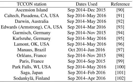
The TCCON validation dataset contained 32,175 OCO-2 measurements taken from 17 Septem-ber 2014 to 2 May 2016. We co-located the OCO-2 measurements in time and space with the AERONET and TCCON, which were required to both be present and operational at a given site. The co-location criteria was within 1◦ latitude/longitude and +/- 30 minutes and the sites selected for use are shown in Figure 2.1. As TCCON stations are all located on land, only a small fraction of co-located measurements are over water surfaces.

Table 2.1 lists the TCCON sites used in this study. The measurements were selected from a set of OCO-2 “lite" files [89] that had been pre-filtered (see Section 2.3). We then post-processed the

90°W 0° 90°E 60°S 30°S 0° 30°N 60°N

TCCON and AERONET Sites

Figure 2.1:TCCON and AERONET sites used in this study.

retrievals with multiple custom filters in an attempt to remove all scenes contaminated by clouds or aerosols.

Table 2.1:TCCON stations used in this study.

TCCON station Dates Used Reference

Ascension Island Sep 2014–Dec 2015 [90] Caltech, Pasadena, CA, USA Sep 2014–May 2016 [91] Darwin, Australia Sep 2014–May 2016 [92] Edwards (Armstrong), CA, USA Sep 2014–Mar 2016 [93] Garmisch, Germany Sep 2014–Nov 2015 [94] Karlsruhe, Germany Sep 2014–May 2016 [95] Lamont, OK, USA Sep 2014–May 2016 [96] Manaus, Brazil Oct 2014–Jun 2016 [97] Orléans, France Sep 2014–Nov 2015 [98] Paris, France Sep 2014–Sep 2015 [99] Park Falls, WI, USA Sep 2014–May 2016 [100]

Saga, Japan Sep 2014–Feb 2016 [101] Sodankylä, Finland Sep 2014–Apr 2016 [102]

2.2.2

Model Validation Dataset

Besides validation against the highly accurate but sparsely located TCCON, a set of global CO2 models was assembled in order to examine spatial errors. We co-located 30,827 OCO-2 measurements in time and space with a suit of nine global carbon models [9, 25, 31, 103–107]. Only points where all the models agreed to within 1 ppm of XCO2 were used. Work by [60] has shown that using this methodology produces similar error statistics to that of the TCCON validation. The median XCO2 of the nine models for each of the 30,827 measurements was used as the truth metric. The OCO-2 measurements were selected by sorting all the measurements into a 4◦ latitude by 4◦longitude spatial grid and filling all grid boxes with up to 10 observations. This allowed for excellent global coverage while limiting the demand on the available computational resources needed to run the retrievals.

2.3

Filtering and Bias Correction

As OCO-2 struggles with scenes containing clouds and aerosols, multiple strategies are used to try and filter out any scene that is contaminated by scattering particles. For both validation datasets, the O2 A-band Preprocessor (ABP; [71]) and Iterative Maximum A-Posteriori Differ-ential Optical Absorption Spectroscopy (IMAP-DOAS) Preprocessor (IDP; [72]) were applied to every measurement before being selected to run through the retrieval. For each validation set, the approximately 30,000 measurements used in this study were those that had successfully passed through the preprocessors. These measurements were determined to be clear enough to be run through the retrieval. After removing measurements that failed to converge, post-processing filter-ing techniques were applied to remove additional low-quality retrievals that were not screened out by the preprocessors. These filters included the reduced χ2_{, a delta pressure parameter (from ABP),} and the CO2and H2O ratios (from IDP). Thus, all tests are being done on a mostly clear dataset and conclusions cannot be drawn about how these retrieval modifications impact the results if scenes with thick cloud or aerosol layers are present. Additionally, as the TCCON stations are located on land, the final post-filtered TCCON validation dataset only contained land measurements and thus

no conclusions can be made about OCO-2 measurements over ocean for the TCCON validation study.

Despite heavy pre- and post-filtering of the dataset to remove cloud and aerosol layers, no atmospheric column is truly free from scattering particles. Thus, a bias correction is typically applied to the final XCO2 in an attempt to mitigate retrieval errors [60]. In the operational B8 product, considerable effort is put into developing a multi-parameter bias correction that reduces the XCO2 bias against several independent truth metrics. In this work, a single parameter bias correction was selected for each validation dataset for simplicity and to ensure a fair comparison across different setups. Additionally, it is hypothesized that an improved aerosol setup might reduce the need for a complex bias correction. The parameter chosen was that which had the largest correlation with XCO2 error. When comparing to TCCON, the retrieved XCO2 was bias corrected by removing a linear fit between the XCO2error (retrieved XCO2 - TCCON XCO2) and the difference between the retrieved surface pressure and the prior surface pressure (“dp"). This was the most correlated parameter in the majority of our TCCON tests and thus was selected as the bias correction parameter. This parameter is correlated with XCO2 biases because any unparameterized clouds and aerosols in the column can make the retrieval think there is a lower surface pressure than in reality. Thus, bias correcting this mistake out is designed to bring the retrieved surface pressures back to realistic values and can approximately account for the improperly parameterized clouds and aerosols. In the case of the model validation dataset, the bias correction parameter was the solar zenith angle. Physically, this represents the removal of artificial biases induced by longer air masses. The reason why this parameter was selected over dp is that the model dataset has excellent latitudinal coverage and thus the air mass is weighted more than dp. TCCON, however, is spatially limited and thus the air mass dependence is not as prevalent when searching for optimal bias correction parameters.

2.4

Modeled Aerosol Priors

As discussed in Section 1.6.1, the OCO-2 retrieval algorithm has several aerosol parameters in its state vector. The prior values for most of these parameters in B8 are fixed or taken from a monthly MERRA-2 climatology. Here, we discuss several methods in which we test the use of instantaneous, 3D modeled aerosol data as prior information to improve upon the current priors with the hope of increasing the precision and accuracy of the final OCO-2 XCO2 product.

The GEOS-5 Forward Processing for Instrument Teams (GEOS-5 FP-IT; [62]) atmospheric model, created and maintained by the NASA Global Modeling and Assimilation Office, is de-signed specifically for instrument teams in that the entire period (2000-current) is run using the same GEOS-5 version to maintain consistency and avoid any unwanted biases from updates to the model. For this work, GEOS-5 FP-IT version 5.12.4, hereafter referred to as GEOS-5, was co-located in time and space with the OCO-2 measurements. GEOS-5 is on a 0.625◦longitude by 0.5◦ latitude horizontal grid with 72 vertical layers extending to 0.01 hPa with a time-step of 3 hours. The model was linearly interpolated in space and the nearest 3-hour model update was chosen in time. For example, if the OCO-2 measurement was taken at 1900 UTC, the 1800 UTC model run was used. The GEOS-5 aerosol scheme contains 15 different types with up to five different size bins for each type, which we aggregate into five unique types: dust, organic carbon, black carbon, sea salt, sulfate. The aggregation process weights by the typical relative amount of optical depth contributed by each type at 760 nm and uses a typical relative humidity value for the hygroscopic types. Each type has a unique optical properties, including the single-scattering albedo, extinc-tion coefficient, and refractive index. Further details can be found in [49]. GEOS-5 ingests Terra MODIS AOD, Aqua MODIS AOD, and Multi-angle Imaging SpectroRadiometer (MISR; [108]) aerosol information. AERONET measurements are not used for this product as the data latency is unacceptably large. Figure 2.2 shows that GEOS-5 AODs correlate better with AERONET com-pared to both the climatological MERRA-2 AODs and the corresponding retrieved AOD values from OCO-2 B8. Thus, using the model and assigning it some confidence should result in an improved correlation in retrieved OCO-2 AODs compared to AERONET.

0.02 0.05 0.14 0.37 1.0

AERONET AOD

MERRA-2 Climatological AOD

N=104, R=0.04, =0.25

AERONET AOD

OCO-2 Retrieved AOD

N=104, R=0.19, =0.08

AERONET AOD

GEOS-5 AOD

N=104, R=0.74, =0.03

Figure 2.2:Left: MERRA-2 climatological AOD vs. AERONET AOD. Middle: OCO-2 B8 retrieved AOD vs. AERONET AOD. Right: GEOS-5 co-located AOD vs. AERONET AOD. The AERONET AODs are the means of the AODs at 675 nm and 870 nm. Overpass means are plotted.

Our primary hypothesis in this work is that using instantaneous modeled aerosol data as prior information will result in smaller XCO2 errors when compared to the current operational setup that uses a monthly climatology. Figure 2.3 shows the first of the two aerosol types selected when using the MERRA-2 monthly climatology and when using the interpolated GEOS-5 model field. Certain features, such as Saharan dust and biomass burning, are generally realistically placed in the clima-tology but the day-to-day variations of the atmosphere are not present and thus the climaclima-tology is not representative of the true state of the atmosphere for a given OCO-2 measurement location. For example, dust is selected over large portions of the high northern latitudes in the GEOS-5 model field, but rarely in the MERRA-2 monthly climatology.

Three methods of varying complexity were chosen to ingest the instantaneous model data:

• Using the top two aerosol types and their corresponding AODs

• Using the top two aerosol types and fitting the amplitude, mean, and variance of a Gaussian distribution to the modeled vertical profile of both types

• Using the top two aerosol types and solving for a scale factor on an interpolated 20-layer modeled aerosol profile

90°W 0° 90°E 60°S 30°S 0° 30°N 60°N 90°W 0° 90°E 60°S 30°S 0° 30°N 60°N DU SS BC OC SU

Figure 2.3: Top: primary aerosol type selected for the month of July using the MERRA-2 climatology. Bottom: primary GEOS-5 aerosol type selected for 1 July 2016 0Z. Aerosol types are dust (DU), sea salt (SS), black carbon (BC), organic carbon (OC), and sulfate (SU).

The methodology for selecting which two (of the five) aerosol types to be included in the state vector is simply sorting them by AOD at 760 nm and selecting the two largest values. The ice cloud, water cloud, and stratospheric aerosol type were always retrieved. The ice cloud and water cloud characteristics were kept the same as B8, while the stratospheric aerosol’s optical depth prior and corresponding uncertainty were determined by our setups described below.

2.4.1

Types and Optical Depths

The first method simply takes the top two aerosol types based on sorting by each type’s AOD and uses their corresponding AODs as prior information for each type. This method is the simplest of our tests and does not rely on any modeled vertical aerosol information.

2.4.2

Types and Gaussian Fits

The second method takes the largest two aerosol types, as before. The 72-layer GEOS-5 aerosol profiles for both types are then interpolated onto the 20-layer OCO-2 vertical grid. The amplitude, mean, and variance of a Gaussian curve are then fit to that 20-layer profile and the amplitude (optical depth), height, and width of that Gaussian are fed in to the retrieval as prior information. An example is shown in Figure 2.4. Occasionally, the fit is a poor representation of the vertical profile. This is often the case with the sulfate type, which can have both a lower tropospheric peak and a stratospheric peak, resulting in a profile that cannot be represented with a single Gaussian. To avoid this issue, the sulfate type, if selected, was fit to below 400 hPa and the stratospheric aerosol type (discussed in Section 1.6.1) was a separate Gaussian fit for the profile above 400 hPa. This method was chosen to test the hypothesis that ingesting vertical information from the model will lead to an improved parameterization of the scattering and, subsequently, a more accurate XCO2.

2.4.3

Types and Scale Factors

The third and most complex method takes the largest two aerosol types sorted by AOD, as before. The 72-layer GEOS-5 aerosol profiles for both types are then interpolated onto the 20-layer OCO-2 vertical grid. A scale factor applied to the interpolated profile is then solved for

0.00000 0.00006 BC 0 200 400 600 800 Pressure [hPa] 0.0000 0.0015 DU 0 200 400 600 800 Pressure [hPa] 0.00000 0.00015 OC 0 200 400 600 800 Pressure [hPa] 0.0000 0.0005 SU 0 200 400 600 800 Pressure [hPa] 0.0000 0.0004 SS 0 200 400 600 800 Pressure [hPa]

Figure 2.4:Example of fitting Gaussians to the GEOS-5 AOD profiles. Upper row is black carbon (black), dust (yellow), and organic carbon (green). Lower row is sulfate (orange) and sea salt (blue). Dashed grey lines are the Gaussian fits to the profiles.