ADVANCED CONTROL OF CONVERTERS WITH MULTITASK
FUNCTIONALITIES IN DISTRIBUTION GRID SYSTEMS
BASED ON CONSERVATIVE POWER THEORY
by Ali Mortezaei
© Copyright by Ali Mortezaei, 2018
ii
A thesis submitted to the Faculty and the Board of Trustees of the Colorado School of Mines in partial fulfillment of the requirements for the degree of Doctor of Philosophy (Electrical Engineering). Golden, Colorado Date ____________________ Signed: _________________________ Ali Mortezaei Signed: _________________________ Prof. Marcelo G. Simoes Doctoral Advisor
Golden, Colorado
Date _____________________
Signed: _________________________ Dr. Dan Knauss Acting Department Head Department of Electrical Engineering
iii ABSTRACT
Distributed generation (DG) play a very important role in the modernization of electric power systems, it is estimated their increasing share of operation in the near future. In addition, there is growing concern on the environmental issues, lack of transmission capacity and limitation in constructing new lines, and increasing demand of energy, that would support a more flexible inverter control, capable of interacting users with the utility grid. The main objective of such a system is providing active power, which is the primary use to balance loads. However, power electronic systems can provide power quality improvement and DG systems would then be used as multi-functional compensators for improving power quality, instead of only balancing or selling active power to the grids. In this context, this dissertation first studies the well-known instantaneous current decomposition theories highlighting the important contributions based on the Instantaneous Power (PQ) theory and the Conservative Power Theory (CPT) and presents a comprehensive comparison from performance and computational complexity perspectives. Although these theories are quite distinct in their formulations, the central idea is to make a comparative study between the current portions and their respective portions of power, in order to show the similarities and divergences between them in terms of characterization of the physical phenomena and in terms of disturbing current compensation. The studied instantaneous current decomposition techniques are then used to provide selective functionalities in distribution systems. Therefore, it is possible to inject active power plus compensate selectively unwanted current terms (reactive, unbalance, and distortion), enabling full exploitation of the inverter capability and increasing its overall cost-benefit and efficiency. Afterwards, control structures with multitask functionality to the grid side converter of the renewables to carry out the power quality ancillary services in the distribution system are developed. The key diversity of the methodologies we proposed in this project with respect to others in the literature is that the developed control structures on the grid side converters are based on the CPT theory. This choice provides decoupled power and current references for the grid side inverter control, which offers very flexible, selective and powerful functionalities. These qualities make the system to be the benchmark for achieving 100% renewable and sustainable grid with multifunctional capabilities. This thesis then proposes the coordinated control of the aforementioned multifunctional interfacing DG systems to enhance the operation of microgrid systems. Based on our proposed method, a hybrid cooperative strategy
iv
is developed that overcomes limitations in communication-based and non-communication-based approaches for the coordinated operation of multifunctional distributed generators in islanded microgrid systems. Two important issues that are addressed are the power quality and undesirable current sharing, particularly in the low-voltage distribution network, where electronic devices are drawing distorted and unbalanced currents. The interactions of such current disturbances with high feeder/line impedances, in a low voltage system cause considerable voltage deterioration and possibly affect sensitive loads showing the requirement for power quality enhancement. Finally, this thesis explores the study and implementation of cascaded multilevel converters, in which the primary concepts relating to modulation, structure, and control schemes are detailed. These topologies are composed of series-connected H-bridge converters with isolated DC links. Therefore, it is possible to integrate renewable energy and storage resources to power grids. The experimental findings validate the applicability and performance of the proposed control strategies in distribution grid systems.
v
TABLE OF CONTENTS
ABSTRACT….. ... iii
LIST OF FIGURES ... viii
LIST OF TABLES ...xiii
ACKNOWLEDGMENTS... xiv
CHAPTER 1 INTRODUCTION ... 1
1.1 Research Objectives ... 3
1.2 Organization of the Thesis ... 4
CHAPTER 2 POWER THEORIES FOR CURRENT DECOMPOSITIONS AND RELATED DEFINITIONS ... 6
2.1 Instantaneous Power Theory (PQ) ... 7
2.1.1 The Clarke Transformation ... 8
2.1.2 The Instantaneous Powers of the PQ Theory ... 9
2.1.3 Power Terms based on PQ theory ... 14
2.2 Conservative Power Theory ... 15
2.2.1 Conservative Power Terms under Periodic Non-sinusoidal Operation ... 15
2.2.2 Current Terms under Periodic Non-Sinusoidal Operation ... 17
2.2.3 Power Terms under Periodic, Non-sinusoidal Operation ... 21
2.2.4 Load Conformity Factors ... 22
2.3 Analysis of Different Compensation Strategies by Means Of Ideal Current Source Models ... 24
2.3.1 Symmetrical and Sinusoidal Voltage Source ... 25
2.3.2 Asymmetrical and Sinusoidal Voltage Source ... 30
2.3.3 Symmetrical and Non-sinusoidal Voltage Source ... 33
2.4 Analysis of Different Compensation Strategies by Means of Three-Phase Three-Wire Inverter ... 35
2.4.1 Compensating Load Current Components Based on CPT: ... 38
2.4.2 Compensating Load Current Components Based on PQ: ... 41
vi
2.6 Discussions ... 45
CHAPTER 3 STUDY OF FOUR-LEG GRID-TIED INVERTER WITH LOCAL POWER SOURCE AND SIMULTANEOUS FUNCTIONALITY ... 46
3.1 Fundamental Formulas ... 47
3.2 The Current Decomposition of the CPT in Single-Phase System ... 48
3.2.1 The Active Current ... 49
3.2.2 Reactive Current ... 49
3.2.3 Void Current ... 50
3.3 Current Decomposition of the CPT in Three-Phase Systems ... 50
3.3.1 Three-Phase Active Current ... 51
3.3.2 Three-Phase Reactive Current ... 51
3.3.3 Three-Phase Void Current ... 51
3.3.4 Three-Phase Balanced Active Current ... 51
3.3.5 Three-Phase Unbalanced Active Current ... 52
3.3.6 Three-Phase Balanced Reactive Current ... 53
3.3.7 Three-Phase Unbalanced Reactive Current ... 53
3.3.8 Compensation of Unbalanced Load ... 54
3.4 Three-Phase Four-Leg Grid-Tied Inverter Structure and Control ... 54
3.4.1 Four-Wire DG Inverter Control Strategy ... 56
3.4.2 Analysis of Different Compensation Strategies by Means of Three-Phase Four-Leg Inverter ... 65
3.5 Discussions ... 72
CHAPTER 4 COORDINATED OPERATION OF MULTIFUNCTIONAL DISTRIBUTED GENERATORS IN A MULTI-INVERTER BASED ISLANDED MICROGRID ... 74
4.1 Cooperative Control of Four-Leg Interfacing Converters in Islanded Microgrid with Power Quality Enhancement Based on CPT Theory ... 76
4.1.1 Microgrid Structure with Four-Leg Interfacing Converters ... 77
4.1.2 Load Current Sharing Strategy among DG Inverter Units ... 86
vii
4.2 Participation of Single-Phase Interfacing Converters in Three-Phase Islanded
Microgrids with Power Quality Enhancement Based on CPT Theory ... 98
4.2.1 Microgrid Structure with Participation of Single-phase Interfacing Converters ... 98
4.2.2 Load Current Components Sharing among Single-Phase and Three-Phase DG Inverters ... 101
4.2.3 Application Examples by Means of Single-Phase and Three-Phase Inverters ... 102
4.3 Discussions ... 108
CHAPTER 5 CASCADED MULTILEVEL CONVERTER FOR POWER QUALITY IMPROVEMENT IN SMARTGRID APPLICATIONS ... 110
5.1 Cascaded H-bridge Multilevel Converter Topology ... 111
5.2 SAPF CHMI Modulation and Control ... 113
5.2.1 Control Strategy ... 116
5.2.2 Analysis of Different Compensation Strategies by Means of Experimental Results ... 123
5.3 Discussions ... 134
CHAPTER 6 CONCLUSIONS AND FUTURE WORK ... 136
6.1 Conclusions ... 136
6.2 Future Work ... 138
6.2.1 Development of Cooperative Control Strategies for Maintenance of Power Quality Indexes in Microgrids with Multiple Bus Considerations ... 138
6.2.2 Development of Bidirectonal Electric Vehicle (EV) Charging System for Smart Grid Applications ... 139
6.2.3 Study of Energy Management System for Smart Microgrids ... 139
viii
LIST OF FIGURES
Figure 2-1 Three-phase three-wire circuit with nonlinear and unbalanced load. ... 24
Figure 2-2 PCC voltages and currents before compensation with symmetrical and sinusoidal voltage sources... 25
Figure 2-3 Unbalanced currents compensation using CPT... 26
Figure 2-4 Void currents compensation using CPT. ... 27
Figure 2-5 Unbalanced and void currents compensation using CPT. ... 28
Figure 2-6 Non active currents compensation using CPT. ... 28
Figure 2-7 Load oscillating active current compensation using PQ. ... 29
Figure 2-8 Load oscillating reactive current compensation using PQ. ... 30
Figure 2-9 PCC voltages and currents before compensation with unbalanced voltage source. ... 31
Figure 2-10 Non active currents compensation (CPT). ... 31
Figure 2-11 Compensation of oscillating active and total reactive currents (PQ). ... 32
Figure 2-12 PCC voltages and currents before compensation with symmetrical non-sinusoidal voltage sources. ... 33
Figure 2-13 Non active currents compensation (CPT). ... 33
Figure 2-14 Non active currents compensation (CPT). ... 34
Figure 2-15 Compensation of oscillating active current and the total reactive current (PQ). .... 35
Figure 2-16 Prototype hardware implementation. ... 36
Figure 2-17 Three-phase inverter configuration. ... 37
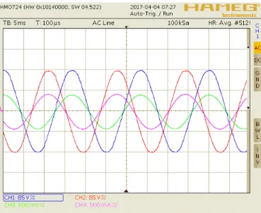
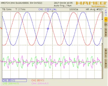
Figure 2-18 Before implementing any compensation strategy: PCC voltage (85 V/div) and load current (5 A/div) of phases a and b. ... 38
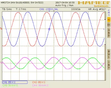
Figure 2-19 Compensation of balanced reactive current component: PCC voltage (85 V/div) and inverter current (0.5 A/div) of phases a and b... 39
Figure 2-20 Compensation of unbalance current component: PCC voltage (85 V/div) and inverter current (0.5 A/div) of phases a and b. ... 39
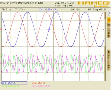
Figure 2-21 Compensation of void current component: PCC voltage (85 V/div) and inverter current (2 A/div) of phases a and b. ... 40
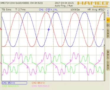
Figure 2-22 Compensation of unbalance and void current components: PCC voltage (85 V/div) and inverter current (2 A/div) of phases a and b. ... 41
ix
Figure 2-23 Compensation of balanced reactive, unbalance, and void current components:
PCC voltage (85 V/div) and grid current (5 A/div) of phases a and b. ... 41
Figure 2-24 Compensation of load constant reactive current component: PCC voltage (85 V/div) and inverter current (0.5 A/div) of phases a and b. ... 42
Figure 2-25 Compensation of oscillatory active current component: PCC voltage (85 V/div) and inverter current (2 A/div) of phases a and b. ... 42
Figure 2-26 Compensation of oscillatory reactive current component: PCC voltage (85 V/div) and inverter current (2 A/div) of phases a and b. ... 43
Figure 2-27 Compensation of oscillatory active and reactive current components: PCC voltage (85 V/div) and inverter current (2 A/div) of phases a and b. ... 43
Figure 3-1 Implementation of active current given by (3.8). ... 49
Figure 3-2 Implementation of reactive current given by (3.9). ... 50
Figure 3-3 Implementation of void current given by (3.10). ... 50
Figure 3-4 Implementation of balanced active current given by (3.15). ... 52
Figure 3-5 Implementation of unbalanced active current given by (3.16). ... 53
Figure 3-6 Considered grid-tied four-leg inverter with a current source modeled as DG. ... 54
Figure 3-7 Four-wire four-leg grid-tied PEI. ... 56
Figure 3-8 Block diagram of the current control loop. ... 57
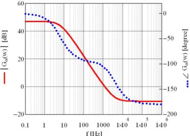
Figure 3-9 Bode diagram of the current control plant in both “𝒔” and “𝒘” planes: (a) Magnitude response, (b) Phase response. ... 58
Figure 3-10 Bode plot of the open loop current transfer function. ... 60
Figure 3-11 Block diagram of the DC voltage control loop. ... 62
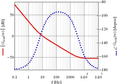
Figure 3-12 Bode plot of the open loop DC-link voltage transfer function. ... 64
Figure 3-13 Active power delivery: (a) PCC voltage and inverter current, (b) PCC voltage and grid current, (c) grid neutral current and inverter neutral current. ... 66
Figure 3-14 Active and reactive power delivery: (a) PCC voltage and inverter current, (b) PCC voltage and grid current, (c) grid neutral current and inverter neutral current. ... 68
Figure 3-15 Active power delivery and reactive and unbalance compensation: (a) PCC voltage and inverter currents, (b) PCC voltage and grid current, (c) grid neutral current and inverter neutral current. ... 69
Figure 3-16 Active power delivery and non-active compensation: (a) PCC voltage and inverter currents, (b) PCC voltage and grid current, (c) grid neutral current and inverter neutral current. ... 70
x
Figure 3-17 PCC conformity factors under multifunctional mode of operation. ... 71
Figure 3-18 Active power delivery and non-active compensation at t=0.5s. ... 72
Figure 4-1 Proposed multi-master-slave-based autonomous microgrid, including groups, A, B, C, D, etc. ... 78
Figure 4-2 Block diagram of the current control scheme. ... 80
Figure 4-3 Bode plot of the open loop current transfer function. ... 82
Figure 4-4 Block diagram of the voltage control scheme. ... 82
Figure 4-5 Simplified dual loop block diagram and flow graph. ... 83
Figure 4-6 Open loop voltage transfer function frequency response. ... 85
Figure 4-7 Schematic diagram of the evaluated multi-inverter-based autonomous microgrid. ... 88
Figure 4-8 Schematic diagram of the configurable load. ... 89
Figure 4-9 Group A and B master inverters voltage waveforms before and after load bus voltage enhancement (t=0.3s). ... 90
Figure 4-10 Group A load bus voltage and current and the current waveforms in each inverter before and after load bus voltage enhancement (t=0.3s). ... 91
Figure 4-11 Group B load bus voltage and current and the current waveforms in each inverter before and after load bus voltage enhancement (t=0.3s). ... 92
Figure 4-12 Group A Load power components. ... 93
Figure 4-13 Group B Load power components. ... 94
Figure 4-14 Active power sharing. ... 94
Figure 4-15 Reactive power sharing. ... 96
Figure 4-16 Unbalance power sharing. ... 97
Figure 4-17 Distortion power sharing. ... 97
Figure 4-18 Schematic diagram of the group A LV Microgrid with the participation of single-phase VSI units ... 99
Figure 4-19 Schematic diagram of the configurable load in groups A and B, (a) block diagram of load A in group A; (b) block diagram of load B in group B. ... 100
Figure 4-20 Group A current waveforms before and after compensation of load non-active current components (t=0.6s). ... 103
Figure 4-21 Group B current waveforms before and after compensation of load non-active current components (t=0.6s). ... 104
xi
Figure 4-22 Group A and B master inverters voltage waveforms before and after
compensation of load non-active current components (t=0.6s). ... 106 Figure 4-23 Groups A and B load buses voltage waveforms before and after compensation
of load non-active current components (t=0.6s). ... 106 Figure 4-24 Active power sharing among VSI units ... 107 Figure 5-1 CHMI Topology. ... 111 Figure 5-2 Block diagram of the power circuit, control scheme, and loads to the power
grid. ... 114 Figure 5-3 Reference and carrier signals for one phase of the 7-level CHMI. ... 115 Figure 5-4 DSP implementation of the PS-PWM for the 7-level CHMI. ... 115 Figure 5-5 Block diagram of the proposed control scheme with DC voltage controllers of
H-bridge cells in phase a ... 117 Figure 5-6 Bode plot of the open-loop current transfer function. ... 120 Figure 5-7 Bode plot of the open loop DC-link voltage transfer function. ... 123 Figure 5-8 Before implementing any compensation strategy: PCC voltage (90 V/div) and
grid current (40 A/div) of phases a and b. ... 124 Figure 5-9 Compensation of balanced reactive current component: CHMI terminal
voltage (110 V/div) and inverter current (5 A/div) of phases a and b, (b) Compensation of balanced reactive current component: PCC voltage (90 V/div) and grid current (40 A/div) of phases a and b. ... 125 Figure 5-10 (a) Compensation of unbalance current component: CHMI terminal voltage
(110 V/div) and inverter current (5 A/div) of phases a and b, (b)
Compensation of unbalance current component: PCC voltage (90 V/div) and grid current (40 A/div) of phases a and b ... 126 Figure 5-11 (a) Compensation of void current component: CHMI terminal voltage
(110 V/div) and inverter current (5 A/div) of phases a and b, (f) Compensation of void current component: PCC voltage (90 V/div) and grid current (40 A/div) of phases a and b. ... 127 Figure 5-12 Compensation of non-active current component under symmetrical and
sinusoidal voltage sourc: (a) PCC voltage (90 V/div) and grid current (40 A/div), (b) CHMI terminal voltages (110 V/div), (c) H-bridge DC-link regulated voltages (25 V/div) of phase a and DC-link current (12 A/div) of H-bridge a1. ... 129 Figure 5-13 Compensation of non-active current component under asymmetrical and
sinusoidal voltage source: (a) PCC voltage (90 V/div) and grid current (40 A/div), (b) CHMI terminal voltages (110 V/div), (c) H-bridge DC-link
xii
regulated voltages (25 V/div) of phase a and DC-link current (12 A/div) of H-bridge a1. ... 131 Figure 5-14 Compensation of non-active current component under symmetrical and
non-sinusoidal voltage source: (a) PCC voltage (90 V/div) and grid current (40 A/div), (b) CHMI terminal voltages (110 V/div), (c) H-bridge DC-link regulated voltages (25 V/div) of phase a and DC-link current (12 A/div) of H-bridge a1. ... 133
xiii
LIST OF TABLES
Table 2-1 Source voltages, line impedance and load parameters. ... 25
Table 2-2 Three-phase Inverter and load parameters. ... 37
Table 2-3 Required mathematical operations and dynamic response for each control method. ... 44
Table 3-1 Three-phase Four-leg Inverter and load parameters. ... 55
Table 3-2 Requirements chosen for current control scheme. ... 59
Table 3-3 Requirements chosen for DC voltage control scheme. ... 63
Table 4-1 Microgrid Inverters Parameters. ... 79
Table 4-2 Requirements chosen for current control scheme. ... 81
Table 4-3 Requirements chosen for voltage control scheme. ... 85
Table 4-4 Load and Line Impedance parameters. ... 89
Table 4-5 Load and Line Impedance parameters. ... 100
Table 5-1 CHMI parameters. ... 117
Table 5-2 Requirements chosen for current control scheme. ... 119
Table 5-3 Requirements chosen for DC voltage control scheme. ... 122
Table 5-4 Load parameters. ... 123
Table 5-5 PCC Power Components, Inverter and Grid Currents, and Power Factor under possible selective compensation strategies. ... 127
Table 5-6 PCC Power Components, Inverter and Grid Currents and Power Factor through the non-active compensation - Case 1. ... 130
Table 5-7 PCC Power Components, Inverter and Grid Currents and Power Factor through the non-active compensation - Case 2. ... 132
Table 5-8 PCC Power Components, Inverter and Grid Currents and Power Factor through the non-active compensation - Case 3. ... 134
xiv
ACKNOWLEDGMENTS
There are many people whom I am indebted to during my Ph.D. study. They have helped me in numerous ways that have enabled this dissertation to come into being. First, and foremost, I wish to thank my supervisor, Dr. Marcelo Godoy Simoes, for giving me valuable guidance throughout the course of my study. His deep insights and positive manner have always been helpful and encouraging. I am also grateful to Dr. Ahmed Al Durra and Dr. S. M. Muyeen from PI for the continuous support of my Ph.D. study and related research. Next, special thanks go to my committee members, Dr. Cristian Ciobanu, Dr. Abd A. Arkadan, and Dr. Pankaj Sen for their time and support, particularly for their patience in reading my draft dissertation. Their advice and assistance are highly appreciated. I would also like to give special thanks to Dr. Fernando P. Marafão, Dr. Tiago D. C. Busarelo, and Dr. Helmo K. M. Paredes who inspired me in the field of power theories. The friendly academic discussions on power quality issues made my study very productive and interesting. I would like to give special thanks to my previous colleagues Mr. Xuliang Hou and Mr. Varaprasad Oruganti who helped and supported me during PhD work.
I would like to express my gratitude to the Colorado School of Mines for bestowing me with a PhD scholarship so that I can continue my research interest in the field of energy systems and power electronics. In addition, I wish to thank Dr. Salman Mohagheghi, Dr. Kathryn Johnson, Dr. Sudipta Chakraborty, Dr. Abdullah Bubshait, Dr. Bananeh Ansari, Dr. Enio Ribeiro, Dr. Mohammad Babakmehr, Dr. Farnaz Harirchi, Mr. Moein Choobineh, Mr. Abdulhakee Alsaleem, Mr. Faleh Alskran, and Ms. Sepideh Kianbakht for their company, friendship, and help.
I am also grateful to Dr. Mohamad Abdul-Hak, Ms. Grace Liu, Dr. Baha Hafez, and Dr. Pirooz Javanbakht from Mercedes Benz Research and Development North America (MBRDNA) for the their support during my one year internship program on electric vehicle charging systems.
Last, but not least, I would like to take this limited space to express my gratitude to my family for their consistent help, support, and in particular, moral support in the journey of my academic career.
xv
This is dedicated to My family, My dear Mom and Dad, for their boundless support and love
1
CHAPTER 1 INTRODUCTION
The world is at the edge of a major shift in the paradigm of electrical energy generation, transmission, distribution and storage, by moving from existing, centralized generation towards distribution energy resources (DER). The new paradigm has the potential to result in higher stability margins and better reliability, reduction of transmission lines power loss, power quality increase, ability to shift peak loads, etc. Smart grid technologies help utilities to operate, control, and maintain DER as well as interconnect them to the main grid. In the new paradigm of the grid, the complexity of technical tasks have changed from dealing with local SCADA data into a variety of massive field data collection, that allows a more comprehensive view of the power system status, energy flows, hierarchical control, asset management, equipment conditions etc. A Microgrid is a localized grouping of DER and loads that has the capability of islanding and operating independently from the grid as well as grid-connected mode of operation. As long as a microgrid is connected to a large grid, the voltage is supported by the main grid and power source connected to the microgrid could generate independently. In contrast, in the islanded operation of microgrids and in electrical islands such as shipboard distribution systems, dynamics are strongly dependent on the connected sources and on the power regulation control of the grid interfacing converters. This may affect control accuracy and stability of the system. Furthermore, load variation has an adverse impact on the quality of voltage. While any load step generally affects the magnitude of voltages at the load bus, nonlinear and unbalanced loads cause distortion and imbalance of the load voltage.
Smart technologies bring about the possibility of a smart microgrid. A smart microgrid typically integrates the following components [1], [2].
1) Renewable energy resources capable of supplying local demand as well as feeding the unused energy back to the electric grid.
2) A variety of loads, including residential, office and industrial loads.
3) Local and distributed power storage units to smooth out the intermittent performance of renewable energy sources.
2
4) Smart meters and sensors capable of measuring electric parameters such as active power, reactive power, voltage, current, harmonics, unbalanced current, and so on with acceptable precision and accuracy.
5) Communication infrastructure that enables system components to exchange information and commands securely and reliably.
6) Smart terminations, loads, and appliances capable of communicating their status and accepting commands to adjust and control their performance and service level based on user and/or utility requirements.
7) A supervisory control, composed of integrated networking, computing, and communication infrastructure elements, that appears to users in the form of an Energy Management System that allows command and control on all nodes of the network.
In many cases the energy sources in a microgrid are interfaced through power electronic converters feeding harvested power to grid. The loads are also connected to the microgrid. Most of the loads are non-linear in nature which draws non-sinusoidal currents distorting the voltage at the point of common coupling (PCC). To solve this problem, another converter is connected in parallel to the load to reduce the harmonic distortion in the grid currents. This extra inverter circuit is called Power Factor Correction (PFC) circuits. Such PFC circuits are referred as typical active power filters. For a typical user, who has his/her own renewable energy sources and his/her own residential loads, needs two parallel connected inverter for the operation of overall system and the cost of the overall system increases. A higher degree of controllability of converters allows for the possibility of ancillary functions for power quality improvement when converters have unused capacity. This calls for a multi-task converter to supplying the load components and mitigating the electrical disturbances existing on the load currents. This work presents flexible control strategies for Distributed generation (DG) units in microgrids to supply selectively the load current components allowing the DG system to inject its available energy, as well as to work as an active power filter, mitigating load current disturbances and improving power quality. In order to avoid instability in the system and to increase the efficiency of the microgrid operation, a coordinated operation between converters in a microgrid is required. Several methods for DGs power control have been proposed, which can be mainly classified as two types: communication-based and non-communication-based control strategies. In case of short distances, it is reasonable to use a communication link among DG inverters with potential improvement in controllability and
3
dynamic response and, consequently, in PCC voltage regulation and proper power sharing [3]. However, there are some drawbacks in communication-based approach, such as the requirement for high-bandwidth communication links, which can be an unfeasible and costly solution for microgrids with long distances among the inverters. Long distance communication lines get interfered easier, therefore, reducing system reliability and expandability [3]. However, communication links should be always an enhanced technical solution, since they have the potential to provide better controllability and better load sharing response [4]. Therefore, a proper coordination scheme should be developed in order to meet the operating criteria of the microgrid such as power flow control, voltage support and harmonic mitigation and unbalance compensation. 1.1 Research Objectives
This project aims at broadly developing an advance control technique of DC/AC converters for integration of DG resources as microgrid system. The proposed control technique can:
1) Connect DG resources to the ac grid via two-level and multilevel converters. 2) Supply load power components with accurate and fast dynamic response. 3) Inject the available active power of DG resources to the microgrid continuously. 4) Mitigate load reactive power and increase the power factor of power grid. 5) Mitigate load harmonic current components.
6) Guarantee balanced overall grid currents of unbalanced load. 7) Provide fast dynamic response in tracking rapid variations in load.
8) Regulate load voltage/frequency in a wide range of load conditions in islanded mode of operation.
9) Control distributed power sources in a microgrid in coordination with each other in order to meet the requirements for the electrical network and overcome these challenges.
Note that in AC microgrids, there are four major power components, i.e. active, reactive, harmonic, and unbalance components that need to be coordinated. For DC microgrids, there is only one power component to control i.e. active component which results in simplicity of the control system compared with the AC microgrid case. Therefore, a power sharing scheme should be developed so that the potential of each DG could be exploited at most.
4
To be fulfilled, the above objectives need to evolve and builds upon a number of tasks. Key tasks are:
1) Development of a supervisory control system for monitoring and measuring loads currents and voltages at PCCs.
2) Development of power electronic interfaces for injection of current/power components under the connection of DG resources to the microgrid.
3) Development of novel reference generation methods for the DG interfacing unit for setting appropriate references of DG control loop circuit.
4) Development of novel current control methods for the DG electronic interface system capable of high power quality current injection of the grid under the presence of grid current distortion, interfacing parameter variation, and converter system delays.
5) Development of novel voltage control methods for the DG electronic interface system capable of fast voltage regulation and effective mitigation of dynamic voltage disturbances.
6) Development of a coordinated operation system for controlling power components among power electronic interfaces for comprehensive duty sharing in the microgrid.
1.2 Organization of the Thesis
This thesis presents a multi-objective control technique of two level and multilevel converter topologies for microgrid operation of distributed generation resources based on renewable energy (and non-renewable energy) resources. The proposed control technique of DG interfacing system is used to improve the quality of power by injection of different current components during integration of DG resources.
Chapter 2 investigates the main similarities and discrepancies among important current decompositions proposed for the compensation of disturbances such as reactive current, asymmetry, unbalances or nonlinearities. Such decompositions and related definitions may influence the power measurement techniques, revenue metering, instrumentation technology and also power conditioning strategies.
Chapter 3 investigates control strategies on the grid side converters of renewable to compensate disturbances caused in presence of reactive, non-linear and/or unbalanced single- and intra-phase loads, in addition to providing active/real power from energy sources. The proposed control
5
methodology provides decoupled power and current references based on the Conservative Power Theory concept to perform power injection and power conditioning simultaneously offering very flexible, selective and powerful functionalities.
Chapter 4 proposes a platform that enables the coordinated operation of multifunctional distributed generators, aiming at making proper use of DG inverter units’ capability to improve power quality indices at microgrid load buses. In this platform, a multi-master-slave-based control of DGs is proposed in which slaves inject the available energy and compensate selectively unwanted current components of local loads with the secondary effect of having enhanced voltage waveforms while masters share the remaining load power autonomously with distant groups using frequency droop.
Chapters 5 investigate the cascaded multilevel converter topology to provide flexible power conditioning for selective compensation or minimization of particular load disturbances in medium voltage systems. The feature of modularity increases the reliability of the device, making this topology an attractive choice for new applications with enhanced energy efficiency and system reliability.
6
CHAPTER 2 POWER THEORIES FOR CURRENT DECOMPOSITIONS AND RELATED DEFINITIONS
Electronic systems and several nonlinear loads are being increasingly used since the advent of power electronics. Such devices are usually more efficient and flexible in a wide range of applications, such as AC and DC motor drives, battery chargers, power supplies, UPS, rectifiers and so on. However, the current quality deterioration due harmonic pollution of switching devices has been increasingly penetrating the utility grid and causing great concerns for the utility companies, operators, and even regular consumers in the local grid [5], [6].
In order to eliminate these harmonics in the electric system, a variety of compensation algorithms were proposed by researches for switching compensators over the last two decades. These compensation algorithms are derived from electric-power theories that are defined in the frequency domain or in the time domain. The conventional active (P), reactive (Q) and apparent (S) powers, defined in the frequency domain [7]–[9], originally in single-phase circuits and then expanded for three-phase circuits, and several other power quality indices that are derived from them are precise only for off-line calculation and analysis of power quality issues. In general, power definitions in the time domain offer a more appropriate basis for the use in controllers for power electronic devices, because they are also valid during transients. This is especially true if the definitions are done considering already a three-phase circuit instead of considering single-phase circuits and then summing up to have a three-phase system [7].
At the beginning [10], two important approaches to power definitions under non-sinusoidal conditions were introduced by Budeanu in 1927 [9], and Fryze in 1932 [11]. Budeanu worked in the frequency domain, whereas Fryze defined the power in the time domain. In 1983 Akagi, Kanazawa and Nabae proposed a time domain power theory for three-phase circuit for the control of active filters connected to three-phase three-wire systems [12]. This theory is known today as PQ theory [7], [10]. In the literature it can be found other power definitions defined in the time domain. The most important are the Fryze-Buchholz-Depenbrock (FBD) proposed by Depenbrock, [13], the Conservative Power Theory (CPT) proposed by Tenti [14], and the CPC (Current’s Physical Components) proposed by Czarnecki, [15], [16]. Also in the literature we can find p-q theory inspired control algorithms for switching compensators as, for example, the p-q-r theory [17]–[19], which is also defined in the 𝛼𝛽0 reference frame. A comparison involving the
7
p-q-r and the p-q theories is provided in [19]. The control method denominated as Synchronous Reference Frame (SRF) [20] also presents similar aspects related with the p-q-r and the p-q theories. The SRF method is defined in the 𝑑𝑞0 reference frame. All of these control algorithms and methods can be applied to control switching compensators connected in three-phase systems, with or without neutral wire. Control algorithms derived from the p-q theory have been widely applied to control switching compensators, and their control algorithms, are well established in the electrical engineering community involved in switching compensators design [7], [10]. However, the PQ theory faces some conceptual problems when it is considered as a power theory for understanding the power properties of the load under non sinusoidal and unbalanced conditions [7], [14], [15], [21]–[24]. It occurs when the real and imaginary currents, derived from the p-q theory, are compared with the active and non-active currents defined by Fryze in 1932 [11].
In this chapter, the main similarities and discrepancies among two important time domain power theories named the instantaneous power (PQ) theory and Conservative Power Theory (CPT) control methods for the compensation of disturbances such as reactive current, asymmetry, unbalances or nonlinearities in the three-phase circuits are studied and a comprehensive comparison from performance and computational complexity perspectives is presented. Although these theories are quite distinct in their formulations, the central idea is to make a comparative study between the current portions and their respective portions of power, in order to show the similarities and divergences between them in terms of characterization of the physical phenomena and in terms of disturbing current compensation. In addition to analyzing performance of different compensation techniques, the computational burden related to the mathematical structure of each technique is also evaluated. A clear understanding of computation burden of each technique helps to choose a technique over another when the computational resources are limited, or select a proper microcontroller for a certain application. Next sections present a concise review of the investigated power theories and related current decompositions. Simulation and experimental results for several cases are discussed and compared in order to point out the major similarities and divergences under different voltage conditions.
2.1 Instantaneous Power Theory (PQ)
The instantaneous real and imaginary power theory (PQ Theory) was published in the IEEE Transactions on Industry Applications in 1984 [25]. The PQ Theory defines a set of instantaneous
8
powers in time domain. Since no restrictions are imposed on voltage or current behaviors, it is applicable to three-phase systems with or without neutral conductor, as well as to generic voltage and current waveforms. Thus, it is valid for steady and transient states.
Other traditional concepts of powers are characterized by treating a three-phase system as three single-phase circuits. The PQ theory firstly transforms voltages and currents from the 𝑎𝑏𝑐 to 𝛼𝛽0 coordinates, and then defines instantaneous powers on these coordinates. Hence, this theory always considers the three-phase system as a unity, and has the advantage of instantaneously separating homopolar (zero-sequence) from nonhomopolar (positive and negative-sequence) components, which may be present in the instantaneous three-phase four-wire voltages and currents. Indeed, since their instantaneous powers are defined in the 𝛼𝛽0 reference frame, it is possible to extract, separately, the homopolar (zero-sequence) component. The PQ theory also allows a comprehensible explanation as to why imaginary power can be compensated without the need of energy storage elements [10], [26]. Besides, it also allows determining the amount of energy that must be stored in a compensation device, in order to compensate oscillating powers that are exchanged between source and load [25], [27].
2.1.1 The Clarke Transformation
The 𝛼𝛽0 transformation or the Clarke transformation maps the three-phase instantaneous voltages in the 𝑎𝑏𝑐 phases, 𝑣𝑎, 𝑣𝑏, and 𝑣𝑐, into the instantaneous voltages on the 𝛼𝛽0 axes 𝑣𝛼, 𝑣𝛽, and 𝑣0. The Clarke Transformation and its inverse transformation of three-phase generic voltages are given by:
[ 𝑣0 𝑣𝛼 𝑣𝛽 ] = √23 [ 1 √2 1 √2 1 √2 1 −12 −12 0 √32 −√32] [𝑣𝑣𝑎𝑏 𝑣𝑐 ] [𝑣𝑣𝑎𝑏 𝑣𝑐 ] = √23 [ 1 √2 1 0 1 √2 − 1 2 √3 2 1 √2 − 1 2 − √3 2] [ 𝑣0 𝑣𝛼 𝑣𝛽 ] (2.1)
Similarly, The Clarke Transformation and its inverse transformation of three-phase generic instantaneous line currents, 𝑖𝑎, 𝑖𝑏, and 𝑖𝑐 are given by (2.2). One advantage of applying the 𝛼𝛽0 transformation is to separate zero-sequence components from the 𝑎𝑏𝑐 phase components. The 𝛼 and 𝛽 axes make no contribution to zero-sequence components.
9 [𝑖𝑖𝛼0 𝑖𝛽 ] = √23 [ 1 √2 1 √2 1 √2 1 −12 −12 0 √32 −√32] [𝑖𝑖𝑎𝑏 𝑖𝑐 ] [𝑖𝑖𝑎𝑏 𝑖𝑐 ] = √23 [ 1 √2 1 0 1 √2 − 1 2 √3 2 1 √2 − 1 2 − √3 2] [𝑖𝑖0𝛼 𝑖𝛽 ] (2.2)
No zero-sequence current exists in a three phase, three-wire system, so that 𝑖0 can be eliminated from the above equations, thus resulting in simplification. If the three-phase voltages are balanced in a four wire system, no zero-sequence voltage is present, so that 𝑣0 can be eliminated. However, when zero-sequence voltage and current components are present, the complete transformation has to be considered.
If 𝑣0 can be eliminated from the transformation matrixes, the Clarke transformation and its inverse transformation become:
[𝑣𝑣𝛼𝛽] = √23[1 − 1 2 − 1 2 0 √32 −√32] [ 𝑣𝑎 𝑣𝑏 𝑣𝑐 ] [𝑣𝑣𝑎𝑏 𝑣𝑐 ] = √23 [ 1 0 −12 √32 −12 −√32] [𝑣𝑣𝛼𝛽] (2.3)
Similar equations hold in the line currents.
2.1.2 The Instantaneous Powers of the PQ Theory
The PQ Theory is defined in three-phase systems with or without a neutral conductor. Three instantaneous powers-the instantaneous zero-sequence power (𝑝0), the instantaneous real power (𝑝), and the instantaneous imaginary power (𝑞) are defined from the instantaneous phase voltages and line currents on the 𝛼𝛽0 axes as [7]:
[𝑝𝑝0 𝑞] = [ 𝑣0 0 0 0 𝑣𝛼 𝑣𝛽 0 𝑣𝛽 − 𝑣𝛼 ] [𝑖𝑖𝛼0 𝑖𝛽 ] 𝑝 = 𝑣𝛼𝑖𝛼+ 𝑣𝛽𝑖𝛽 = 𝑝̅ + 𝑝̃ 𝑞 = 𝑣𝛽𝑖𝛼− 𝑣𝛼𝑖𝛽 == 𝑞̅ + 𝑞̃ 𝑝0 = 𝑣0 𝑖0 = 𝑝̅0+ 𝑝̃0 (2.4)
where, “−” represents the average and “~” represents the oscillating components of each power. It is important to point out that differently from other power definitions, the powers defined in (2.4) considers all three-phase voltages and currents. In theories presented in [7], [13]–[16], the definitions are based on single phase voltage and current and therefore do not allow the understanding of what is possible to have with definitions in three-phases voltages and currents as in the PQ theory.
10
The physical meanings of the instantaneous powers defined in the 𝛼𝛽0 reference frame, including their average and oscillating components are described as follow. The instantaneous real power (𝑝) represents the energy, per time unity, that flows from the source to the load (or from the load to the source, if negative) through the three phase wires [10], [28]. The average component of the real power (𝑝̅), if positive, constitutes the energy, per time unity, that is transferred from the source to the load. The oscillating component (𝑝̃) corresponds to the energy, per time unit, that is exchanged between the source and the load.
In three-phase electrical circuits (with or without neutral wire) where voltages and currents are only comprised by their fundamental positive-sequence components, the energy transfer is unidirectional, normally from the source to the load. In this case, the instantaneous real power (𝑝) contains only its average component (𝑝̅). There are also others particular situations in which energy can present a unidirectional transfer from the source to the load as, for example, when voltages and currents present the same harmonic components and; moreover, present the same symmetrical components (positive, negative or zero components). In any other situations, where the voltages and currents are composed by distorted or unbalanced components, the instantaneous real power presents average and oscillating components.
The instantaneous zero-sequence power (𝑝0) results from zero-sequence components of voltages and currents (𝑣0) and (𝑖0). It is important to comment that this power only exists in three-phase circuits with neutral wire. The average component (𝑝̅0) corresponds to the energy, per time unity, that flows from the source to the load using the neutral wire. The oscillating component (𝑝̃0) corresponds to the energy flow, per time unity, that is exchanged between source and load through the neutral wire. It is important to notice that the average component cannot exist without the presence of oscillating one [10].
The instantaneous three-phase active power (𝑝3𝜙), determined in 𝑎𝑏𝑐 coordinates, and the instantaneous real power (𝑝) and instantaneous zero-sequence power (𝑝0), determined in 𝛼𝛽0 coordinates, can be associated as follows [7]:
𝑝3𝜙 = 𝑣𝑎𝑖𝑎+ 𝑣𝑏𝑖𝑏+ 𝑣𝑐𝑖𝑐 = 𝑣𝛼𝑖𝛼+ 𝑣𝛽𝑖𝛽+ 𝑣0𝑖0 = 𝑝 + 𝑝0 (2.5)
There are no zero-sequence current components in three phase three-wire systems, that is 𝑖0 =
11
𝑣0𝑖0 is zero. Hence, in three-phase three wire systems, the instantaneous real power represents the
total energy flow per time unity, in terms of 𝛼𝛽 components. In this case, (𝑝3𝜙 = 𝑝). In an electrical system composed by voltages and currents with fundamental positive-sequence components only, it is possible to assure that the instantaneous three-phase active power (𝑝3𝜙) and the instantaneous real power (𝑝) are equal, presenting only average component (𝑝̅). Moreover, as described in [10], [28], [29], in this condition is also possible to affirm that the conventional active power (𝑃) is equal to the instantaneous powers (𝑝3𝜙) and (𝑝). In any other condition, the active power (𝑃) corresponds only to the average component of the instantaneous active power (𝑝3𝜙).
It is important to note that the conventional power theory defined reactive power as a component of the instantaneous (active) power, which has an average value equal to zero. Here, the instantaneous imaginary power (𝑞) can be understood as responsible for the energy, per time unit, that is exchanged between the three-phase wires of the electrical system. Therefore, the power that flows in each phase and depends on (𝑞) does not contribute to the energy that flows from the source to the load or vice-versa. The instantaneous three phase reactive power (𝑞3𝜙), determined in 𝑎𝑏𝑐 coordinates, and the imaginary power can be associated as follows [7]:
𝑞3𝜙 = (𝑣𝑎− 𝑣𝑏)𝑖𝑐+ (𝑣𝑏− 𝑣𝑐)𝑖𝑎+ (𝑣𝑐 − 𝑣𝑎)𝑖𝑏 = √3(𝑣𝛽𝑖𝛼− 𝑣𝛼𝑖𝛽) = √3𝑞 (2.6)
The instantaneous reactive power (𝑞3𝜙) is similar to the conventional reactive power (𝑄) only when the fundamental positive-sequence components of the voltages and currents are considered. When the currents or voltages present harmonic or unbalanced components, the instantaneous power (𝑞3𝜙) contains average and oscillating components, which makes impossible to compare (𝑞3𝜙) with (𝑄).
Based on the aforementioned explanations involving the real, imaginary and zero-sequence powers, the authors of PQ theory conclude that [7]:
The total energy that flows per time unity, that is, the instantaneous three-phase active power is always equal to the sum of the real and zero-sequence powers.
In phase circuits, with or without neutral wire, it is possible to affirm that the three-phase active power (𝑝3𝜙) is equal to the conventional active power (𝑃), if the voltages and
12
currents are only comprised by their fundamental positive-sequence (or only negative-sequence) components.
The instantaneous imaginary power is only derived from the nonhomopolar components of the voltages and currents. Moreover, there is a power in each phase that depends on the imaginary power, but their three-phase instantaneous sum is always equal to zero.
Based on the real and imaginary powers, together with the phase voltages transformed to 𝛼 and 𝛽 components, it is possible to determine a set of real and imaginary current currents corresponding to these powers. This is very suitable for better explaining the meaning of the powers defined in the PQ Theory. From (2.4), it is possible to write [7]:
[𝑖𝑖𝛼 𝛽] = 1 𝑣𝛼2 + 𝑣𝛽2[ 𝑣𝛼 𝑣𝛽 𝑣𝛽 −𝑣𝛼] [ 𝑝 𝑞] =𝑣𝛼2+ 𝑣1 𝛽2[ 𝑣𝛼 𝑣𝛽 𝑣𝛽 −𝑣𝛼] [𝑝0] +𝑣 1 𝛼2+ 𝑣𝛽2[ 𝑣𝛼 𝑣𝛽 𝑣𝛽 −𝑣𝛼] [0𝑞] = [ 𝑖𝛼𝑝 𝑖𝛽𝑝] + [ 𝑖𝛼𝑞 𝑖𝛽𝑞] (2.7)
The above current components can be defined as shown below. Instantaneous real current on the 𝛼 axis 𝑖𝛼𝑝:
𝑖𝛼𝑝 = 𝑣 𝑣𝛼
𝛼2+ 𝑣𝛽2𝑝
(2.8)
Instantaneous imaginary current on the 𝛼 axis 𝑖𝛼𝑞:
𝑖𝛼𝑞 = 𝑣 𝑣𝛽
𝛼2+ 𝑣𝛽2𝑞
(2.9)
Instantaneous real current on the 𝛽 axis 𝑖𝛽𝑝:
𝑖𝛽𝑝 =𝑣 𝑣𝛽
𝛼2+ 𝑣𝛽2𝑝
(2.10)
Instantaneous imaginary current on the 𝛽 axis 𝑖𝛽𝑞: 𝑖𝛽𝑞 =𝑣 −𝑣𝛼
𝛼2+ 𝑣𝛽2𝑞
(2.11)
Accordingly, the 𝑎𝑏𝑐 real currents, the 𝑎𝑏𝑐 imaginary currents, and zero-sequence currents can be determined by using the same procedure as the below:
13
The 𝑎𝑏𝑐 real currents can be determined applying the appropriate inverse Clarke transformation on the real currents as follow:
[ 𝑖𝑎𝑝 𝑖𝑏𝑝 𝑖𝑐𝑝 ] = √23 [ 1 √2 1 0 1 √2 − 1 2 √3 2 1 √2 − 1 2 − √3 2 ] [ 0 𝑖𝛼𝑝 𝑖𝛽𝑝 ] = √23 [ 1 0 −12 √32 −12 −√32 ] [𝑖𝑖𝛼𝑝 𝛽𝑝] (2.12)
The 𝑎𝑏𝑐 imaginary currents can be determined applying the appropriate inverse Clarke transformation on the real currents as follow:
[ 𝑖𝑎𝑞 𝑖𝑏𝑞 𝑖𝑐𝑞 ] = √23 [ 1 √2 1 0 1 √2 − 1 2 √3 2 1 √2 − 1 2 − √3 2 ] [ 0 𝑖𝛼𝑞 𝑖𝛽𝑞 ] = √23 [ 1 0 −12 √32 −12 −√32 ] [𝑖𝑖𝛼𝑞 𝛽𝑞] (2.13)
The 𝑎𝑏𝑐 zero-sequence currents can be determined applying the appropriate inverse Clarke transformation on the real currents as follow:
[𝑖𝑖𝑎0𝑏0 𝑖𝑐0 ] = √23 [ 1 √2 1 0 1 √2 − 1 2 √3 2 1 √2 − 1 2 − √3 2 ] [𝑖00 0] = 1 √3[ 𝑖0 𝑖0 𝑖0 ] (2.14)
So, the instantaneous three-phase currents (a, b and c) can be decomposed on the following components: [𝑖𝑖𝑎𝑏 𝑖𝑐 ] = [𝑖𝑖𝑎0𝑏0 𝑖𝑐0 ] + [ 𝑖𝑎𝑝 𝑖𝑏𝑝 𝑖𝑐𝑝 ] + [ 𝑖𝑎𝑞 𝑖𝑏𝑞 𝑖𝑐𝑞 ] (2.15)
14 2.1.3 Power Terms based on PQ theory
The instantaneous power on the α and β coordinates are defined as 𝑝𝛼 and 𝑝𝛽, respectively,
and are calculated from the instantaneous voltages and currents on the αβ axes as follows [7]: [𝑝𝑝𝛽𝛼] = [𝑣𝑣𝛼𝑖𝛼 𝛽𝑖𝛽] = [ 𝑣𝛼𝑖𝛼𝑝 𝑣𝛽𝑖𝛽𝑝] + [ 𝑣𝛼𝑖𝛼𝑞 𝑣𝛽𝑖𝛽𝑞] (2.16)
It was mentioned that in the three-phase, three-wire system, the three-phase instantaneous active power (𝑝3𝜙) in terms of Clarke components is equal to the instantaneous real power (𝑝). The instantaneous real power can be given by the sum of 𝑝𝛼 and 𝑝𝛽. Therefore, rewriting this sum yields the following equation:
𝑝 = 𝑣𝛼𝑖𝛼𝑝+ 𝑣𝛽𝑖𝛽𝑝+ 𝑣𝛼𝑖𝛼𝑞+ 𝑣𝛽𝑖𝛽𝑞 =𝑣 𝑣𝛼2 𝛼2+ 𝑣𝛽2𝑝 + 𝑣𝛽2 𝑣𝛼2+ 𝑣𝛽2𝑝 + 𝑣𝛼𝑣𝛽 𝑣𝛼2+ 𝑣𝛽2𝑞 + −𝑣𝛼𝑣𝛽 𝑣𝛼2+ 𝑣𝛽2𝑞 (2.17)
In the above equation, there are two important points. One is that the instantaneous real power is given only by:
𝑣𝛼𝑖𝛼𝑝 + 𝑣𝛽𝑖𝛽𝑝= 𝑝𝛼𝑝 + 𝑝𝛽𝑝 = 𝑝 (2.18)
The other is that the following relation exists for the terms dependent on 𝑞:
𝑣𝛼𝑖𝛼𝑞+ 𝑣𝛽𝑖𝛽𝑞 = 𝑝𝛼𝑞 + 𝑝𝛽𝑞 = 0 (2.19)
The above equations suggest the separation of the powers in the following types: Instantaneous real power on the α axis 𝑝𝛼𝑝:
𝑝𝛼𝑝 = 𝑣𝛼𝑖𝛼𝑝 = 𝑣𝛼 2
𝑣𝛼2+ 𝑣𝛽2𝑝
(2.20)
Instantaneous imaginary power on the α axis 𝑝𝛼𝑞:
𝑝𝛼𝑞 = 𝑣𝛼𝑖𝛼𝑞 =𝑣 𝑣𝛼𝑣𝛽
𝛼2+ 𝑣𝛽2𝑞
15 Instantaneous real power on the β axis 𝑝𝛽𝑝:
𝑝𝛽𝑝 = 𝑣𝛽𝑖𝛽𝑝 = 𝑣𝛽 2
𝑣𝛼2+ 𝑣𝛽2𝑝
(2.22)
Instantaneous imaginary power on the β axis 𝑝𝛽𝑞:
𝑝𝛽𝑞 = 𝑣𝛽𝑖𝛽𝑞 = 𝑣−𝑣𝛼𝑣𝛽
𝛼2+ 𝑣𝛽2𝑞
(2.23)
The above equations lead to the following important conclusions [7]:
The sum of the α axis instantaneous real power 𝑝𝛼𝑝 and the β axis instantaneous real power 𝑝𝛽𝑝 corresponds to the instantaneous real power 𝑝.
The sum of 𝑝𝛼𝑞 and 𝑝𝛽𝑞 is always zero. Therefore, they do not contribute to the instantaneous
nor average energy flow between the source and the load in a three phase circuit. This is the reason that they were named instantaneous imaginary power on the α and β axes. The instantaneous imaginary power 𝑞 gives the magnitude of the powers 𝑝𝛼𝑞 and𝑝𝛽𝑞.
Because the sum of 𝑝𝛼𝑞 and 𝑝𝛽𝑞 is always zero, their compensation do not need any energy
storage element.
2.2 Conservative Power Theory
The Conservative Power Theory (CPT), proposed by Tenti et al. and recently reformulated in [30] is defined in time domain for any operating conditions and it can be applied in polyphase systems, with or without return conductor. The CPT theory proposes power and current’s decomposition in the stationary frame, according to terms which are directly related to electrical characteristics, such as: average power transfer, reactive energy, unbalanced loads and nonlinearities. The basic definitions are recalled hereafter, while additional information can be found in previous publications [30]–[32].
2.2.1 Conservative Power Terms under Periodic Non-sinusoidal Operation
Assuming a generic poly-phase circuit under periodic operation (period 𝑇), where (𝑣) and (𝑖) are, respectively, the voltage and current vectors and (𝑣̂) is the unbiased integral of the voltage vector measured at a given network port (phase variables are indicated with subscript “𝑚”), the following terms were defined:
16 Active power: 𝑃 = 𝑝̅ = 〈𝑣, 𝑖〉 =𝑇 ∫ 𝑣 ∙ 𝑖 𝑑𝑡 = ∑ 𝑃1 𝑚 𝑀 𝑚=1 𝑇 0 (2.24)
Instantaneous active power:
𝑝 = 𝑣 ∙ 𝑖 = ∑ 𝑣𝑚𝑖𝑚 𝑀
𝑚=1
(2.25)
The active power equals to the average value of the instantaneous active power and represents the average power flowing through the port and it coincides with the conventional definitions. As known, the value of 𝑃 does not depend on the voltage reference. Moreover, the active power is a conservative quantity, i.e., it is additive over all network components.
The active power, which corresponds to the average power consumption, is not enough to characterize the network operation, not even in case of passive linear circuits. Power fluctuations and current flows caused by energy storage elements must be also taken into account, and under sinusoidal conditions, this phenomenon is accounted by reactive power 𝑄, which is also conservative and independent of voltage reference.
Extending the reactive power concept to periodic non-sinusoidal operation, the CPT makes reference to reactive energy 𝑊 in the following form [30]:
Reactive energy: 𝑊 = 𝑤̅ = 〈𝑣̂, 𝑖〉 =𝑇 ∫ 𝑣̂ ∙ 𝑖 𝑑𝑡 = ∑ 𝑊1 𝑚 𝑀 𝑚=1 𝑇 0 (2.26)
Instantaneous reactive energy:
𝑤 = 𝑣̂ ∙ 𝑖 = ∑ 𝑣̂𝑚𝑖𝑚 𝑀
𝑚=1
(2.27)
Reactive energy is the average value of Instantaneous reactive energy. It is a new quantity which is related to the average energy conveyed through the port. Moreover, the instantaneous reactive energy is a time function, which requires the integration of the phase voltages. In here, (𝑣̂) is the vector of unbiased integral of the port voltages. Reactive energy 𝑊 is a conservative quantity for
17
every voltage and current waveform. It can be shown that, due to the Tellegen’s Theorem, the instantaneous quantities and their average values are conservative for whichever network and irrespective of voltage and current waveforms [30], [32]. This is not generally true for conventional reactive power definitions.
It is worth noting that definitions (2.24) to (2.27) hold irrespective of voltage and current waveforms provided that they are periodic. Moreover, computation of the quantities defined by (2.24) to (2.27) is directly done in the time domain and requires integration and low-pass filtering only. Finally, since the conservation property holds in general, active power and reactive energy are additive quantities in every electrical network. It is important to highlight that under sinusoidal conditions the terms 𝑝 and 𝑤 coincides at any time with the conventional active (𝑃𝑐𝑜𝑛𝑣 = 𝑉𝐼 cos 𝜑) and reactive powers (𝑄𝑐𝑜𝑛𝑣= 𝜔𝑊 = 𝑉𝐼 sin 𝜑), with 𝜑 being the displacement angle
and 𝜔 being the grid frequency [30], [32].
Another relevant, though not conservative, power term characterizing the network operation at a given port is the apparent power 𝐴 = 𝑉𝐼 where 𝑉 and 𝐼 are the collective RMS values of phase voltages and currents and are expressed by the following equations where 𝑀 is the number of phases and the summation does not include the neutral wire.
𝑉 = √〈𝑣, 𝑣〉 = √∑𝑀𝑚=1𝑉𝑚2, 𝐼 = √〈𝑖, 𝑖〉 = √∑𝑀𝑚=1𝐼𝑚2 (2.28)
2.2.2 Current Terms under Periodic Non-Sinusoidal Operation
The phase currents are decomposed into three basic current components explained below. Basic Current Terms
Consider a generic port of a 𝑀-phase network and let 𝑣𝑚 and 𝑖𝑚 be the voltage and current
measured at phase 𝑚 terminals. We decompose current in order to identify the terms related to active power 𝑃𝑚 and reactive energy 𝑊𝑚 absorbed by phase 𝑚 at the given port [30].
2.2.2.1.1 Active Current
The active current is the minimum phase current (i.e., with minimum RMS value) needed to convey active power 𝑃𝑚. It is expressed by:
18 𝑖𝑎𝑚 = 〈𝑣‖𝑣𝑚, 𝑖𝑚〉 𝑚‖2 𝑣𝑚 = 𝑃𝑚 𝑉𝑚2𝑣𝑚 = 𝐺𝑚𝑣𝑚, 𝑚 = 1,2, … 𝑀 → 𝐼𝑎 = √∑ 𝐼𝑎𝑚2 𝑀 𝑚=1 = √∑ (𝑃𝑉𝑚 𝑚) 2 𝑀 𝑚=1 (2.29)
In (2.29), term 𝐺𝑚 = 𝑃𝑚⁄𝑉𝑚2 is the equivalent conductance of phase 𝑚. The active current has no impact on reactive energy, as it can easily be shown from (2.29).
2.2.2.1.2 Reactive Current
The reactive current is the minimum phase current needed to convey reactive energy 𝑊𝑚. It is expressed by: 𝑖𝑟𝑚 =〈𝑣̂‖𝑣̂𝑚, 𝑖𝑚〉 𝑚‖2 𝑣̂𝑚 = 𝑊𝑚 𝑉̂𝑚2 𝑣̂𝑚 = ℬ𝑚𝑣̂𝑚, 𝑚 = 1,2, … 𝑀 → 𝐼𝑟 = √∑ 𝐼𝑟𝑚2 𝑀 𝑚=1 = √∑ (𝑊𝑚 𝑉̂𝑚) 2 𝑀 𝑚=1 (2.30)
In (2.30), term 𝐵𝑚 = 𝑊𝑚⁄ is the equivalent reactivity of phase 𝑚. The reactive current has 𝑉̂𝑚2
no impact on active power, as it can easily be shown from (2.30). 2.2.2.1.3 Void Current
The remaining current term is called void current and is not conveying active power and reactive energy. It is defined by:
𝑖𝑣𝑚 = 𝑖𝑚− 𝑖𝑎𝑚− 𝑖𝑟𝑚, 𝑚 = 1,2, … 𝑀 (2.31)
2.2.2.1.4 Orthogonality
All the aforementioned current terms are orthogonal, thus:
19
Note that active and reactive currents refer to power and energy terms that are conservative in every network and also keep their meaning in presence of distortion, voltage asymmetry, and load unbalance.
Balanced Current Terms
As for conventional networks under sinusoidal operation, it makes sense to identify the effects of supply voltage asymmetry and load unbalance, because they both affect power quality. Of course, under non-sinusoidal operation, the traditional approach must be revised and this can easily be done based on the earlier definitions. Notice, first of all, that we use term “unbalance” to characterize the load attitude to perform asymmetrically in the different phases. Instead, term “asymmetry” is associated to an asymmetrical behavior of the supply seen from load terminals. Irrespective of supply asymmetry, load unbalance, and waveform distortion, the following current terms is defined.
2.2.2.2.1 Balanced Active Currents
The balanced active currents are the minimum currents (i.e., with minimum collective RMS value) needed to convey total active power 𝑃 = ∑𝑀𝑚=1𝑃𝑚 absorbed at the network port. They are given by: 𝑖𝑎𝑏= 〈𝑣, 𝑖〉 ‖𝑣‖2𝑣 = 𝑃 𝑉2𝑣 = 𝐺𝑏𝑣 → 𝐼𝑎𝑏 = 𝑃 𝑉2 (2.33)
In (2.33), coefficient 𝐺𝑏 = 𝑃 𝑉⁄ is the equivalent balanced conductance. Note that these 2
currents are the same that would be absorbed by a symmetrical resistive load with same active power consumption as the actual load. Also, note that the balanced active currents track phase voltages (𝑣) irrespective of their waveform. Thus, these currents are symmetrical only if the phase voltages are symmetrical. The term “balanced” therefore refers to load symmetry, not to current symmetry.
2.2.2.2.2 Balanced Reactive Currents
Similarly, the balanced reactive currents are the currents with minimum collective RMS value needed to convey total reactive energy 𝑊 = ∑𝑀𝑚=1𝑊𝑚 absorbed at the port. They are given by:
20 𝑖𝑟𝑏= 〈𝑣̂, 𝑖〉 ‖𝑣̂‖2𝑣̂ = 𝑊 𝑉̂2𝑣̂ = 𝐵𝑏𝑣̂ → 𝐼𝑟𝑏 = 𝑊 𝑉̂2 (2.34)
In (2.34), coefficient 𝐵𝑏= 𝑊 𝑉̂⁄ is the equivalent balanced reactivity. Note that these currents 2
are the same that would be absorbed by a symmetrical reactive load taking same reactive energy as the actual load. Also, note that the balanced reactive currents track voltage integrals (𝑣̂) irrespective of their waveform. Thus, these currents are symmetrical only if the phase voltages are symmetrical. Additionally, in this case, the term “balanced” therefore refers to load symmetry, not to current symmetry.
Unbalanced Current Terms 2.2.2.3.1 Unbalanced Active Currents
Unbalanced active currents are defined by:
𝑖𝑎𝑢 = 𝑖𝑎− 𝑖𝑎𝑏 → 𝑖𝑎𝑚𝑢 = 𝑖𝑎𝑚− 𝑖𝑎𝑚𝑏 = (𝐺𝑚− 𝐺𝑏)𝑣𝑚, 𝑚 = 1,2, … 𝑀 → 𝐼𝑎𝑢 = √∑ (𝑃𝑉𝑚 𝑚) 2 − (𝑃 𝑉) 2 𝑀 𝑚=1 (2.35)
Clearly, these currents exist only if the load is unbalanced, i.e., if the equivalent phase conductances differ from each other. Note that the balanced and unbalanced active currents are collectively orthogonal, i.e.
〈𝑖𝑎𝑢, 𝑖𝑎𝑏〉 = 0 → 𝐼𝑎𝑢 = √𝐼𝑎2− 𝐼𝑎𝑏2
(2.36)
2.2.2.3.2 Unbalanced Reactive Currents
Similarly, the unbalanced reactive currents are defined by:
21 𝐼𝑟𝑢 = √∑ (𝑊𝑉̂𝑚 𝑚) 2 − (𝑊 𝑉̂) 2 𝑀 𝑚=1
These currents exist only if the equivalent phase reactivities differ from each other. The balanced and unbalanced reactive currents are collectively orthogonal, thus,
〈𝑖𝑟𝑢, 𝑖𝑟𝑏〉 = 0 → 𝐼𝑟𝑢 = √𝐼𝑟2− 𝐼𝑟𝑏2
(2.38)
We collectively refer to unbalance currents as the sum of active and reactive unbalance terms, which are orthogonal each other. Thus,
𝑖𝑢 = 𝑖
𝑎𝑢 + 𝑖𝑟𝑢 → 𝐼𝑢 = √𝐼𝑎𝑢2+ 𝐼𝑟𝑢2
(2.39)
2.2.2.3.3 Complete Current Decomposition
In conclusion, the phase currents can be split as follows:
𝑖 = 𝑖𝑎𝑏+ 𝑖𝑟𝑏+ 𝑖𝑎𝑢+ 𝑖𝑟𝑢+ 𝑖𝑣 = 𝑖𝑎𝑏+ 𝑖𝑛𝑎 (2.40)
such that 𝑖𝑎𝑏 is the balanced active current, 𝑖𝑟𝑏 is the balanced reactive current, 𝑖𝑢 is the unbalance
current, 𝑖𝑣 is the void current, and 𝑖𝑛𝑎 is the non-active current. All terms are orthogonal, thus,
𝐼 = √𝐼𝑎𝑏2+ 𝐼𝑟𝑏2+ 𝐼𝑢2+ 𝐼𝑣2 = √𝐼𝑎𝑏2+ 𝐼𝑛𝑎2
(2.41)
It should be emphasized once more that the earlier definitions are valid, and keep their physical meaning, for whichever voltage and current waveform, supply asymmetry and load unbalance. 2.2.3 Power Terms under Periodic, Non-sinusoidal Operation
From (2.41), the apparent power defined earlier is decomposed as follows [30]:
𝐴 = √𝑉2𝐼𝑎𝑏2+ 𝑉2𝐼𝑟𝑏2+ 𝑉2𝐼𝑢2+ 𝑉2𝐼𝑣2 = √𝑃2+ 𝑄2+ 𝑁2+ 𝐷2 (2.42)
where,
22
𝑄 = 𝑉𝐼𝑟𝑏 is the reactive power (2.42.b)
𝑁 = 𝑉𝐼𝑢 is the unbalance power (2.42.c)
𝐷 = 𝑉𝐼𝑣 is the void power (2.42.d)
The reactive power is related to the balanced reactive currents and consequently to the reactive energy, but the reactive power can be affected by the grid frequency and voltage distortions, as discussed in [30]–[32]. The unbalance power (𝑁 = √𝑁𝑎2 + 𝑁𝑟2) is associated to imbalances on the
phase conductances and reactivities. In the case of single phase circuits, such component vanishes. The distortion power is related to the existence of nonlinear elements or conditions. Additional details can be found in [30]–[32].
2.2.4 Load Conformity Factors
By means of the CPT theory, a set of performance indices based on the orthogonal current/power decomposition can be defined to characterize different aspects of load operation [33], [34]. The general conformity factor is the power factor (𝜆), which can be calculated in any generic circuit, independently to the waveform distortions or asymmetries and represents the global efficiency of the load, under certain voltage supplying conditions. This power factor definition is affected not only by voltage and current displacement, but also by unbalanced and nonlinear loads. Unit power factor represents current waveforms proportional to voltage waveforms (as in case of balanced resistive loads). 𝜆 = 𝐼𝑎𝑏 √𝐼𝑎𝑏2+ 𝐼𝑛𝑎2 = 𝐼𝐼 =𝑎𝑏 𝑃𝐴 = 𝑃 √𝑃2+ 𝑄2+ 𝑁2+ 𝐷2 (2.43)
Of course, under sinusoidal and symmetrical (or single-phase) voltage and current conditions, (𝜆) is equal to the traditional fundamental displacement factor (cos 𝜑), where 𝜑 is the phase angle between fundamental phase voltage and current. However, this relation is not correct if the grid voltages and/or currents are distorted and/or unbalanced.
The reactivity factor (𝜆𝑄) has been defined as: 𝜆𝑄 = 𝐼𝑟 𝑏 √𝐼𝑎𝑏2+ 𝐼𝑟𝑏2 = 𝑄 √𝑃2+ 𝑄2 (2.44)