ff
Value vs. Growth Stocks
Do Value Stocks Outperform Growth Stocks?
Stockholm Stock Markets, 1995-2009
Södertörns högskola | Institutionen för ekonomi och företagande Kandidat uppsats 7,5 hp | Finansiering | vårterminen 2012Av: Gidi Abadiga Marcel Neibig
SAMMANFATTNING
Denna studie undersöker om en investering i värdeaktier kan generera en bättre avkastning jämfört med en investering i tillväxtaktier.
Historisk data för aktier som handlats på Stockholmsbörsen har sammanställts från diverse källor. Till exempel Börsguide och från databasen Thomson Reuters Ecowin Pro. Med hjälp av denna och övrig relevant historisk sekundärdata har aktier grupperats in i värde- och tillväxtportföljer beroende på deras P/E-tal i fem portföljer med olika köp- och innehavstider som sträcker sig från 12 upp till 60 månader mellan åren 1996 och 2009.
Inom varje innehavstid för de olika portföljerna har antalet av värde- och tillväxtaktier varierat. Från, till exempel, 11 aktier under period ett till 20 aktier under period fem. Aktier har ”köpts” och hållits kvar med en inledande investeringar på 20000 SEK i början av varje portföljs innehavstid med hänsyn till studiens syfte.
Avkastningen för dessa investeringar beräknas med tre olika genomsnittliga avkastningsberäkningar. Årliga medelprisavkastningar, innehavsavkastningar och
riskjusterade avkastningar. Beräkningar har gjorts för årlig innehavsperiod, för hela
innehavsperioden och för alla portföljers innehavsperioder tillsammans. Utifrån resultaten för dessa beräkningar har utvecklingen för värde- och tillväxtaktier analyserats.
När all fem portföljer jämförs tillsammans och den årliga medelvärdesavkastningen beräknats, så genererar värdeaktierna i genomsnitt 15,1 % högre avkastning än tillväxtaktier gällande en årlig genomsnittlig riskjusterad avkastning. Resultatet för innehavsavkastning är i genomsnitt 5,6 % högre än för tillväxtaktierna.
De här resultaten tyder på att en investering i värdeaktier, genom att använda historisk fundamental information, kan generera en bättre avkastning jämfört med tillväxtaktier. Följaktligen kan man försiktigt hävda att Stockholmsbörsen tycks uppvisa egenskaper gällande en semi-stark form av den effektiva marknadshypotesen.
ABSTRACT
This study tries to examine if investment in value stocks (poor performing stocks) can generate superior returns over investment in growth stocks.
Historical stock data for stocks traded in Stockholm stock markets are collected from various sources such as Börsguide and Reuters Thomson Ecowin Pro database. Using these and other relevant secondary historical data, stocks were grouped into value and growth portfolios depending on their P/E-multiples for five buy and hold periods which range from twelve months up to sixty months between investment periods 1996 and 2009.
In each portfolio holding period, different numbers of value and growth stocks, ranging from, for example eleven stocks in period one, to twenty stocks in period five are purchased and held for an initial investment of 20000 SEK at the beginning of each portfolio holding period for the purpose of the study.
The returns to these investments are computed for three different average return
measurements. These are annual Mean Price Returns, Holding Period Returns and Risk-Adjusted Returns for each of the portfolio holding year, for the entire holding periods as well as for the entire portfolio holding periods combined together. Using the spread between these measures, the performances of both value and growth stocks are analyzed.
When all the five portfolios are combined together and the mean annual rate of returns are computed, value stocks outperform growth stocks by an average of 15.1 % mean annual Risk -Adjusted Return Rate. The result for Holding Period Return is an average of 5.6 % higher than the growth stocks.
These results indicate that investment made in value stocks identified using historical fundamental data can generate superior returns than growth stocks. Consequently, it can cautiously be argued that Stockholm stock markets appear to exhibit the characteristics of the semi-strong form of the Efficient Market Hypothesis.
TABLE OF CONTENTS 1. INTRODUCTION... 1 1.1. Background ... 1 1.2. Problem Discussion... 2 1.3. Research Questions... 5 1.4. Purpose... 5 1.5. Perspective ... 6 1.6. Delimiting ... 6 2. THEORETICAL FRAMEWORK ... 7
2.1. Efficient Market Hypothesis (EMH)... 7
2.2. Criticism Against EMH ... 8
2.3. Portfolio Theory... 9
2.3.1. Portfolio Risk and Historical Rate of Return ... 9
2.3.2. OMX Stockholm 30 Index (OMXS 30) ... 11
2.3.3. Risk Adjustment... 11
2.4. Valuation Models and Fundamental Analysis Models ... 12
2.5. Previous Researches... 12
2.5.1. Oertmann- Study in three regions, 18 stock markets... 13
2.5.2. Anderson and Brooks, Study of Long-Term Price-Earnings Ratio (UK)... 13
2.5.3. Fama and French, the International Evidence. ... 14
2.5.4. The Value Premium by Lu Zhang... 14
2.5.5. Summary of the Selected Previous Studies and the Research Frontiers... 15
3. METHOD... 17
3.1. Methodological Approach... 17
3.2. Quantitative Research ... 18
3.3. Data Collection and Portfolio Creation... 19
3.4. Procedures and Steps Used in the Calculation of the Various Returns... 20
3.5. Reliability... 27
3.6. Validity ... 27
3.7. Method Critic... 28
4. RESULTS... 29
4.1. Comparing Value and Growth Portfolio Holding Period Returns (HPR)... 29
4.1.1. HPR vs. Market Index... 31
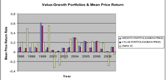
4.2. Comparing Value and Growth Portfolio Mean Price Returns ... 32
4.2.1 Mean Price Return vs. Market Index... 34
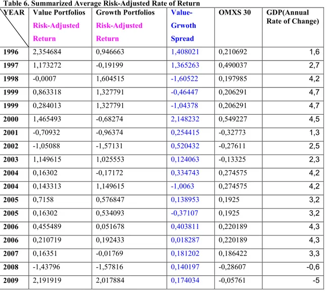
4.3. Comparing Value and Growth Portfolio Risk-Adjusted Returns... 35
4.3.1. Risk-Adjusted Return vs. Market Index... 36
4.4. Comparing Value and Growth Portfolio Returns and Change in GDP... 37
4.4.1 Holding Period Return (HPR) and GDP ... 37
4.4.2 Mean Price Return and GDP ... 38
4.4.3 Risk-Adjusted Rate of Return and GDP... 39
5. ANALYSIS... 40
5.1. Analysis and Discussions... 40
6. CONCLUSIONS and REMARKS... 44
6.1. Conclusion ... 44
6.2. Shortcomings of the Study... 46
6.3. Remarks ... 46
6.4. Recommendations for Further Studies... 47
BIBLIOGRAPHY ... 49
APPENDICES ... 52
Appendix B: Portfolio Data for Period One (1996-01-01 to 1999-09-30)... 53
Appendix C: Portfolio Data for Period Two (1999-10-01 to 2004-09-30) ... 58
Appendix D. Portfolio Data for Period Three (2004-10-01 to 2005-09-30)... 66
Appendix E. Portfolio Data for Period Four (2005-10-01 to 2006-09-30) ... 69
Appendix F. Portfolio Data for Period Five (2006-10- 01 to 2009-12-31)... 72
Appendix G. Risk-Free Rate... 78
Appendix H: OMXS 30 Mean Annual Return 1996 - 2009 ... 80
Appendix I: Annual GDP Volume Change – Production ... 81
TABLE OF FIGURES
FIGURE1. ANNUALCHANGE INGDP 1995-2009... 29
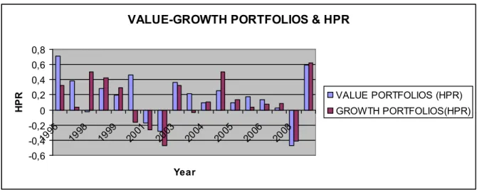
FIGURE2. VALUE-GROWTHANNUALHPR ... 31
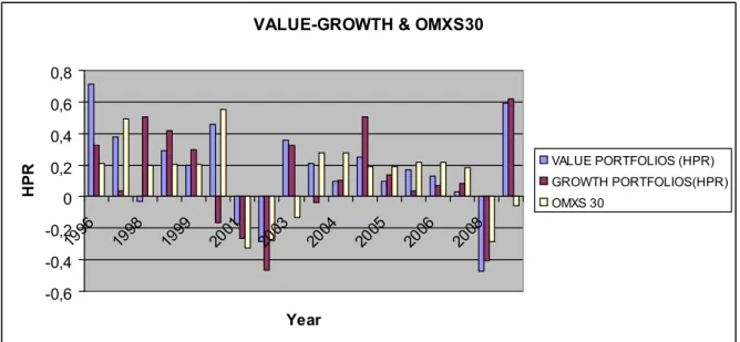
FIGURE3. VALUE-GROWTHHPR & OMXS 30 ... 32
FIGURE4. VALUE-GROWTHANNUALMEANPRICERETURN... 33
FIGURE5. VALUE-GROWTHANNUALMEANPRICERETURN ANDOMX ... 34
FIGURE6. VALUE-GROWTHANNUALRISK-ADJUSTEDRATE OFRETURN... 36
FIGURE7. VALUE-GROWTHRISK-ADJUSTEDRETURN ANDOMXS 30 ... 37
FIGURE8.VALUE-GROWTHHPR ANDANNUALCHANGEINGDP... 38
FIGURE9. VALUE-GROWTHANNUALMEANPRICERETURN ANDGDP ... 38
FIGURE10. VALUE-GROWTHRISK-ADJUSTEDRETURN ANDGDP... 39
LIST OF TABLES
TABLE1. VALUESTOCKSMEANMONTHLYPRICE1996 ... 23
TABLE2. VALUESTOCKSMONTHLYPRICERETURNYEAR1996... 24
TABLE3.VALUESTOCKSMEANMONTHLYRATE OFRETURN1996... 25
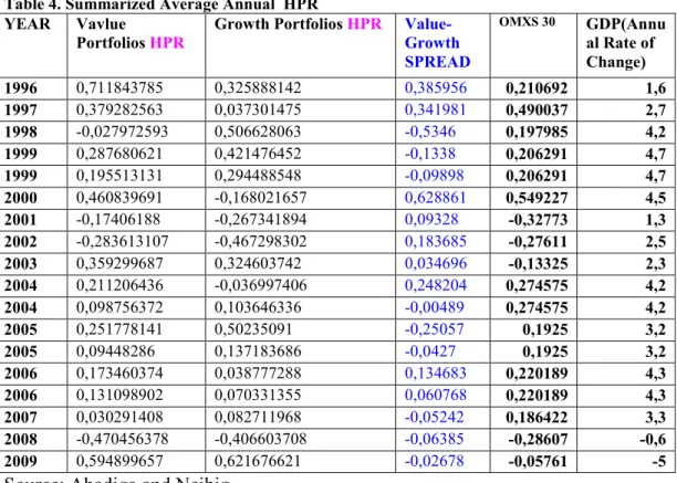
TABLE4. SUMMARIZEDAVERAGEANNUAL HPR... 30
TABLE5. SUMMARIZEDAVERAGEANNUALMEANPRICERETURNS... 32
TABLE6. SUMMARIZEDAVERAGERISK-ADJUSTEDRATE OFRETURN... 35
TABLE7 B. GROWTHSTOCKS1996... 53
TABLE8 B. GROWTHSTOCKS1997... 54
TABLE9B. GROWTHSTOCKS1998... 54
TABLE10B: GROWTHSTOCKS1999... 55
TABLE11B. VALUESTOCKS1996... 55
TABLE12B. VALUESTOCKS1997... 56
TABLE13B. VALUESTOCKS1998... 56
TABLE14B. VALUESTOCKS1999... 57
TABLE15C. GROWTHSTOCKS1999... 58
TABLE16C. GROWTHSTOCKS2000... 58
TABLE17C. GROWTHSTOCKS2001... 59
TABLE18C. GROWTHSTOCKS2002... 60
TABLE19C. GROWTHSTOCK2003... 60
TABLE20C. GROWTHSTOCK2004... 61
TABLE21C. VALUESTOCKS1999... 61
TABLE22C. VALUESTOCKS2000... 62
TABLE23C. VALUESTOCKS2001... 63
TABLE24C. VALUESTOCKS2002... 63
TABLE25C. VALUESTOCKS2003... 64
TABLE26C. VALUESTOCKS2004... 65
TABLE27D. GROWTHSTOCKS2004... 66
TABLE28D. GROWTHSTOCKS2005... 66
TABLE29D. VALUESTOCKS2004... 67
TABLE30D. VALUESTOCKS2005... 68
TABLE31E. GROWTHSTOCKS2005... 69
TABLE32E. GROWTHSTOCKS2006... 69
TABLE33E. VALUESTOCKS2005 ... 70
TABLE34E. VALUESTOCKS2006 ... 71
TABLE35F. GROWTHSTOCKS2006 ... 72
TABLE36F. GROWTHSTOCKS2007 ... 72
TABLE37F. GROWTHSTOCKS2008 ... 73
TABLE38F. GROWTHSTOCKS2009 ... 73
TABLE39F. VALUESTOCKS2006 ... 74
TABLE40F. VALUESTOCKS2007 ... 75
TABLE41F. VALUESTOCKS2008 ... 76
TABLE42F. VALUESTOCKS2009 ... 76
1. INTRODUCTION
This chapter gives an overview of the long-going debate as well as the main actors involved from different camps regarding the efficiency of capital markets in general and the issues revolving around the contentious topic of identifying underperforming stocks and earning superior returns (value premiums) than what other market participants could obtain.
1.1. Background
The desire to improve upon one’s present condition and attain a better station seems a
character shared by at least fairly ambitious human beings. That desire drives each individual at various directions in pursuit of what they might consider a better station in life in their particular ways.
Those who have a gift for enterprise and a taste for excellence in business endeavours purposefully search for opportunities that generate better rewards. One of those areas is investment. Individuals as well as companies engage in the production, distribution and consumption of goods and services in order to gain rewards for their endeavours.
Capital markets have for long been serving this purpose by being one of the major hubs that help pool resources from various corners and facilitate the smooth running of the overall economic activities. Actors in the capital market as much as they expect to get rewards from the normal business activities have also been actively trying to find ways that can help them go a mile a head of the crowd.
One of the techniques that are said to be used on capital markets by certain investors is value investing. Value investing is identifying securities, using fundamental variables, which are deemed underperforming by the market and investing in them and harvesting hefty rewards. Mr Warren Buffett, one of the foremost contemporary proponents of value investing, argues that:
The common intellectual theme of the investors from Graham- and –Doddsville is this: they search for discrepancies between the value of a business and the price of a small piece of that business in the market. Essentially, they exploit these discrepancies without the efficient market theorist’s
concern as to whether the stocks are bought on Monday or Thursday, or whether it is January or July, etc.1
This view, obviously, is not shared by all. There are those, supposedly dominated by academics, who strongly argue against the view that investors can beat the market. They attempt to show that in a market filled by rational and self-interest driven investors, it is impossible to predict the future price movement of securities significantly different from the others and earn hefty returns.
Researches have been conducted at different times and on various markets around the world to reinforce one school or disprove the models and hypothesis of the other. As might be expected in any similar intellectual engagements of merits, both schools seem to continue to thrive with their adherents diligently working to enrich their positions with new supporting evidences and further development of their models that expand the research frontier.
From the modest material search that we have conducted both in the library and online, it seems that there is very little material to indicate that extensive researches have been conducted on this topic on Stockholm stock markets.
This modest study, therefore, is an attempt to take up a few of these research topics and test them against Stockholm stock markets and try to observe how value stocks and growth stocks performed within the selected time period.
1.2. Problem Discussion
The existing economic system and most of the institutions functioning under it appear to get better organized and more complex from time to time. One of these institutions is capital markets.
Despite advances in technologies, accumulation of data and knowledge and countless theories and models that explain their characteristics and functioning , capital markets in particular and the overall economy in general have not yet escaped the tight grips of intermittent abnormal
1Warren E Buffet, ‘The Super investors of Graham-and-Doddsville’, Speech delivered in 1982 at Columbia University, commemorating the fiftieth anniversary of ‘Security Analysis’. Presented as exhibit in Glen Arnold’s Corporate Financial Management, 2nd
tendencies and cyclical fluctuations. Such anomalies continue to guide researchers towards closer examinations and continuous formulation of hypothesis, theories, and models to fully explain the behaviours of both the capital markets as well as the human actors involved in those markets.
The study of the characteristics of the capital market has divided, roughly stating, the academic and investor communities into two schools. While the adherents of EMH strongly argue that the market is efficient, the other school stress that there are at least pockets of inefficiencies that can be identified and the behavioural dimensions of market actors that might lead to inefficiencies or superior returns on investments.2
Eugene Fama, one of the main proponents of the efficient market hypothesis, states that: A market in which firms can make production-investment decisions, and investors can choose among securities that represent ownership of firms’ activities under assumption that security prices at any time ‘fully reflect’ all available information. A market in which prices always ‘fully reflect’ available information is called efficient.3
This hypothesis lays the foundation for the general assertion that prices movements in the capital markets do not follow a given pattern that an investor can study through careful examination of historical data and then be able to predict future price movements. In short, this theory and its predecessor the theory of random walk in stock market prices explain that prices do not follow any pattern but instead make random walk that no one investor can use past prices as the basis to make future price predictions.
In situations where market participants make predictions of the future price movements, the hypothesis clarifies, it is not a single participant but all rational market participants that simultaneously arrive at similar forecasts and hence no one single investor is in a better position to beat the general market for a longer period of time.
This theory is augmented by another economic theory that presupposes market participants as rational agents who always try to maximize their utilities. Consequently, the moment the capital market exhibits a mismatch between prices of securities and incoming relevant
information, these rational investors would immediately seize upon it and drive prices back to
2Chan, Louis, K.C. and Lakonishok, Josef, ‘Value and Growth Investing: A review and Update’, Financial Analysts Journal Vol. 60, No. 1
(Jan. - Feb., 2004), pp 71-86.
their normal levels.4 This, according to the EMH makes it impossible to beat the market for a meaningful length of time and earn above normal or average rates of return on investments with similar levels of risks. Fama further explains the efficiency of capital markets and the behaviour of rational investors as follows:
If the discrepancies between actual prices and intrinsic values are systematic rather than random in nature, then knowledge of this should help intelligent market participants to better predict the path by which actual prices will move towards intrinsic values. When the many intelligent traders attempt to take advantage of this knowledge, however, they will tend to neutralize such systematic behavior in price series.5
Those levels of returns that appear to defy this theory or seen as anomalies, the proponents of EMH explain, are not outcomes of the inefficiency of markets but are results of one or some of the following conditions: sheer luck, the small-firm-in-January effect, the neglected-firm effect, post-earnings-announcement price drift and other related aspects.6
Despite the persuasiveness of the EMH, there is yet another model, which is said to be preferred by professors in universities, in finance that shows security analysis can lead to the identification of overvalued and/or undervalued assets. This model is commonly referred to as Fundamental Securities Analysis Model. It “uses earnings and dividend prospects of the firm, expectations of future interest rates, and risk evaluation of the firm to determine proper stock prices.”7
The categorization of stocks as value and growth is the result of the application of the Fundamental Analysis Model applied upon individual securities. Adherents of this model contend that with due diligence and the inclusion of proper parameters, securities undervalued by the market can be identified and invested in to earn above normal rate of return.
When discussing the efficiency of a capital market, the issue of the dominant firms in the market and their sensitivities to business cycle fluctuations is an aspect that might be considered as it might have a great impact on the results observed.
For example, among the stocks quoted on Nasdaq OMX Nordic, the three most traded large cap companies for trading years 2009 and 2010 were Nokia, Ericson and H&M. The first two
4 Eugene F. Fama, ‘Random Walks in Stock Market Prices’, Financial Analysts Journal, (September-October 1965), p. 56.
5Ibid, pp. 55-59.
6 Zvi Bodie et el., Investments, 7th edn (New York: McGraw-Hill, 2008), p. 363. 7 Ibid.
are technology companies while the third company belongs to retail industry.8 There are no sufficient previous studies that show the effects of the dominance of a given market by
particular industry on the value-growth returns in global markets and it is difficult to find such material on Stockholm stock markets. Since the Stockholm stock market is dominated by technology stocks which are thought to be highly sensitive to business cycle fluctuation, the changes in GDP might have reflected in the performances of both value and growth stocks.
However, a recent study conducted on Canadian market for the period 1985-2005 managed to observe the prevalence of value stocks during both recessions and recoveries even though half the market capitalization was taken up by natural resources and financial services sectors which are assumed to be sensitive to business cycle fluctuations.9
1.3. Research Questions
The study concentrates on the following main questions.
Does a portfolio of value stocks outperform a portfolio of growth stocks? Does a portfolio of value stocks outperform the market index?
Do the relative performances of portfolios of both value and growth stocks remain the same when the GDP decreases and increases?
1.4. Purpose
The purpose of this study is to investigate if investments in value stocks can generate superior returns than investments in growth stocks in Stockholm stock markets. Parallel with that, a study of how portfolios of both value and growth stocks perform when compared to the performance of the OMXS 30 market index is made. Moreover, closer examination of the performances of both value and growth stocks under periods of both rising and falling GDP are conducted. Based on the results of the parameters mentioned above, the study will look at the characteristics of the Stockholm stock markets in the rigour of the Efficient Market Hypothesis and examine which market behaviour is dominantly exhibited.
8Nasdaq OMX, Statistics 2010 the Nasdaq OMX Group (2011-01-04),
http://nordic.nasdaqomxtrader.com/digitalAssets/73/73391_statistics_dec_2010_eur.pdf. (Accessed 2012-04-09)
9George Athanassakos, Value versus Growth Stock Returns and the Value Premium: The Canadian Experience 1985–2005, Canadian
Journal of Administrative Sciences , Revue canadienne des sciences de l’administration 26: 109–121 (2009)
1.5. Perspective
This study is conducted from the perspective of an investor, mainly an institutional investor that has the resources to leave significant mark on the market.
1.6. Delimiting
The study collects historical fundamental data for companies traded in Stockholm stock market from 1995 up to 2009. This is a period for which there is sufficient stock information easily accessible and assumed to be sufficient to make comparison of the performance of both value and growth stocks. Furthermore, the study concentrates on five portfolio holding periods, namely 1996 - 1999, 1999 - 2004, 2004 – 2005, 2005-2006 and 2006 – 2009. These are the periods that have shown significant change in annual GDP growth rate according to GDP data obtained from Statistiska Centralbyrån (Swedish Central Statistics Bureau).
2. THEORETICAL FRAMEWORK
This chapter introduces the relevant theories such as Efficient Market Hypothesis and Portfolio Theory and the main models used in this study such as Fundamental Valuation and Risk-Return calculations Models. Summarized introduction to each of the selected relevant previous studies and a brief overview of the research frontier are also provided.
2.1. Efficient Market Hypothesis (EMH)
This theory is selected because it is one of the basic theories in finance that stipulate that in ideal capital markets there is no way that an investor can identify value stocks that the other market participants have not identified. After additional researches in the field, the hypothesis is further expanded to included three characteristics that describe a capital market. In this study, the results and analysis shall be used to identify the characteristic of Stockholm stock markets according to the behaviours of a market that the EMH postulates.
EMH describes that prices of securities at any time fully reflect all available information. Depending on the nature of information asymmetry that market actors might face, it is divided into strong, semi-strong and weak forms of EMH. When explaining this sub-categorization of the hypothesis, Fama contends that it:
Will serve the useful purpose of allowing us to pinpoint the level of information at which the hypothesis breaks down. And we shall contend that there is no important evidence against the hypothesis in the weak and semi-strong form tests (i.e., prices seem to efficiently adjust to obviously publicly available information), and only limited evidence against the hypothesis in the strong form tests.10
The study tries to use this theory to understand and categorize the characteristics of the Stockholm stock markets. If the Stockholm stock markets are efficient then there would be no significant return on investments in value stocks that are above the market returns. If,
however, value stocks out perform growth stocks it indicates that Stockholm stock markets are not efficient and thus which variants of EMH hypothesis is relevant shall be studied closely.
The weak form:
Weak efficiency - The price follow a random walk. This means that the price reflects all historical information. Investors cannot predict the future price by historical information.11In other words, the weak form of EMH rejects the application of technical analysis.
The semi-strong form:
Semi-strong efficiency refers to the price reflected in all public information. Public
information includes annual accounting reports, stock splits, new stock issues and the likes. One cannot predict a future price using all public information.12
The strong form:
Strong efficiency implies that the price is reflected in all public information and insider information. This means that investors cannot predict the future price of securities using all available information and insider information.13
2.2. Criticism Against EMH
Criticism has been raised against the EMH assertion that investors in the financial markets are rational. Behavioral Finance criticizes EMH by stating that it ignores the way investors make decisions which in turn affects the market. The basic assumption in Behavioral Finance is that people do not act rationally but rather irrationally when making complex decisions. It argues that people do not always interpret and perceive information correctly and therefore make miscalculations, regarding the future returns.14
In summary, there is a wealth of phenomena in Behavioral Finance that acts as
counterarguments against the EMH, in terms of misinterpretation of information. It is said that people have too much confidence in their own abilities that makes them overestimate their knowledge. People make miscalculations because they take too much account of past experience and recent events to predict future occurrences.15 Furthermore, some believe that
people are separating decisions that they rather should combine and that investors are too
11Hillier et al., Corporate Finance, European edn (Berkshire: McGraw-Hill, 2010,) pp.352-353.
12Ibid, pp.353-354.
13Ibid, p.354.
14Bodie et al. Investments, 6th edn (New York: McGraw-Hill, 2005), p.396.
slow to absorb new information, which can lead to a misleading price of a share.16
People’s irrational behavior is the cornerstone of Behavioral Finance which is contrary to EMH argument. Despite the criticisms raised against EMH, the hypothesis remains as a basic assumption among economists and researchers that informs further studies.
2.3. Portfolio Theory
Though this study is based on a posteriori results (realized results), the theory is selected because it explains how investment decisions are made, in the first place. Portfolio theory explains how investors can construct portfolios of assets that meet the level of their risk sensitivities and earn them maximum returns.
It describes how risky securities are priced by relating risk, systematic risk, and the level of expected returns. The ground assumption is that investors calculate the payoffs according to the risk level they are willing to bear when constructing either value or growth stocks.
An important effect of this is that the portfolio total risk can be reduced without producing a lower return. According to Ridder, you must therefore not "put all your eggs in one basket." A portfolio should preferably consist of different securities to reduce risk.17
2.3.1. Portfolio Risk and Historical Rate of Return
Markowitz defines an investment risk in terms of the yield volatility, with the standard deviation as risk measure. The standard deviation calculated from the investment's average deviation from the mean and expressed as a percentage, the same unit for the return. If returns are normally distributed, it shows an indication of the actual return relative to expected
returns.18The standard deviation is also the most important risk measure of price changes for
a security in the financial analysis.19
16
Bodie et al. Investments, 6th edn (New York: McGraw-Hill, 2005), p.398.
17Adri De Ridder , Företaget och de Finansiella Farknaderna, 2nd edn (Stockholm: A. De Ridder , 1996), p.76. 18Ibid, p.77.
To study the behaviour of the return of the two categories of portfolios that have been selected and to compare them with each other as well as with the market index, it is essential to
compute the historical rate of return for value and growth stocks, and the OMXS 30 market index.
When calculating the return of the stocks over time, the formula for Holding Period Return (HPR) is used. HPR takes into account any increase/decrease in stock price plus dividends, if any, where returns are reported in percent. HPR assume that dividends are paid at the end of the holding period.20
HPR = beginning beginning ending price dividend price price
For further calculations of the portfolio return over time, the geometric average return is calculated. This return shows the average increase/decrease in returns over a specified period.21
Geometric Mean Return =
1 1
1 2
...1
11 n n r r r
Risk-Free-Rate: the rate of return one gets by investing on short-term government securities. Due to assumed ability of the government to raise taxes and pay back its debt; these securities are treated as risk-free assets. The study takes historical data about Statsskuldväxlar 3 mån interest rates in computing the performances of the portfolios. Since the study calculates the rate of returns for all portfolios on yearly basis it would have been more appropriate to use the interest rate on government bond with one year maturity but it is not easily to find historical data on such Swedish government bonds.
Equity risk premium is the difference between the rate of return to risky stocks and the risk-free short-term government bonds. This is the reward that an investor gets by investing in risky stocks instead of investing in the risk free government bonds.
20Bodie et al., Investments, 7th edn (New York: McGraw-Hill, 2008), p.124.
2.3.2. OMX Stockholm 30 Index (OMXS 30)
The study uses OMX Stockholm 30 Index. It is selected because it is made up of 30 most actively traded stocks in Stockholm Stock Exchange. Moreover, OMXS 30 is a market weighted index that is reviewed every two years.22 Historical data for OMXS 30 between
1996 and 2009 is collected and used to compare the performances of both value and growth portfolios against the Stockholm stock market during the study period.
2.3.3. Risk Adjustment Sharpe measure: p f r r
measures average portfolio excess return over the sample period
divided by the standard deviation of returns over the period.
This financial calculation is the most popular model for measuring risk-adjusted returns. The return of various portfolios must be risk-adjusted before they can be compared, since different portfolios have varying risks. The Sharpe ratio is a ratio used to calculate the risk-adjusted return on an investment and shows how much return per unit of total risk as the portfolio manager has performed.23
Since investors, according to portfolio theory, want to receive the highest return possible per measurement of risk, this method will be ideal for the purpose of this study.
If a portfolio shows a higher Sharpe ratio, it implies that it has attained a higher risk-adjusted return with a good balance between risk and return. This ratio is calculated by taking the portfolio's return, subtracted by the risk free rate (3 month T-bill) divided by the portfolio's standard deviation.24
The core of this study is to find out if value stocks outperform growth stocks with in the selected study period. Since all investments entail some degree of risk, the returns to those investments can not relatively be judged without taking into consideration those risks. The
22Nasdaq OMX, OMX Stockholm 30, Methodology.
https://indexes.nasdaqomx.com/Data.aspx?IndexSymbol=OMXS30(Accessed 2012-05-02).
23 Bodie et al., Investments, 8th edn (New York: McGraw-Hill, 2009), p.825. 24 Ibid, p. 826.
study is adjusts all returns to their risks and then tries to compare both value and growth stocks and see which one is giving a superior payoff than the other.
2.4. Valuation Models and Fundamental Analysis Models
Dividend discount models (DDM) and Constant-growth dividend discount model (CDDM) are two prominent measures for valuing securities. The DDM is used to get the present price of a security by discounting its dividend payout and future sale value by using this formula.
Specifically, fundamental analysis uses variables such as P/E , price-to-book value (P/BV), market-value-to-book-value (MV/BV), market capitalization, cash-flow-to-price (C/P), and dividend-to-price (Div/P) multiples together with the DDM to identify equities that are undervalued, called value stocks, by the market.
This model is discussed here in order to help the reader appreciate that in a real world investment decision making process, investors make a priori evaluations (expected returns) using these variables to identify value and growth stocks.
Using one variable of the fundamental evaluation model namely price-earning-multiple, the study constructs both value and growth stocks for the five buy and hold portfolio periods.
2.5. Previous Researches
The performance of value stocks over growth stocks has attracted many researchers who attempt to unravel the underlying cause for this phenomenon over the years. At different times and on different markets studies were conducted and testes were performed.
Here attempts are made to recast a few of these studies. Market studied, time period, variables studied and methods employed for sample selection and analysis and results of the studies are summarized below for comparison.
2.5.1. Oertmann- Study in three regions, 18 stock markets25
The study covers 18 stock markets in Europe (including Sweden), North America and the Pacific Rim for the period starting January 1980 up to June 1999. This study categorized companies into value-growth using the previous month-end price-to-book ratios (P/BV). Those with the lowest P/BV, which is half of the market capitalization of the country, fall under value index and the remaining half got categorized as growth index.
Over the study period, the average annual return spread between these two categories account for 1.79 % in Europe, 5.17 % in the Pacific Rim and minus 0.43 % in North America
denominated in local currencies. This shows a significant divergence among the three regions. There is a wide spread for specific countries. For example, in Sweden it was minus 1.84 % while it showed 12.84 % for Norway.
However, overall value stocks earned higher returns than growth stocks for more than two third of the countries.
2.5.2. Anderson and Brooks, Study of Long-Term Price-Earnings Ratio (UK).26
This study examines all UK companies for the period 1975 - 2003 and takes into
consideration many years of Price-Earnings-Ratios to identify stocks as value and growth and see if it has improved effects on returns than what has been observed using a single year P/E-multiple.
It gathers eight years of price-earnings ratios rather than the previous one year many studies used to categorize stocks as value and growth. After that, it divides each category into deciles and calculates the average returns for up to eight years of holding periods.
According to this research, using several years of earning data has reinforced the ability of the P/E-multiple to predicting the return differences between growth and value stocks. This
25
Peter Oertmann, ‘Why do Value Stocks Earn Higher Returns Than Growth Stocks, and Vice Versa?’, Finanzmarket und Portfolio Management, 14 Jahrgang, 2000 , Nr 2 (131-151).
http://www.fmpm.org/files/2000_02_Oertmann.pdf (Accessed: 2012-01-16).
26Anderson, Keith and Brooks, Chris, ‘Long-Term Price-Earnings Ratio’, Journal of Business Finance & Accounting, 33(7) & (8),
approach led them to find that the return difference between value stocks and growth stocks almost doubled.
This study identified that value stocks outperform growth stocks on average annual return of 6 % in the period 1975- 2003 when all UK companies were studied.
2.5.3. Fama and French, the International Evidence.27
This study analysed returns on United States and twelve other countries called EAFE (Europe, Australia, and the Far East) countries.
Portfolios of both value and growth stocks were formed on the basis of such variables as BV/MV, E/P, C/P, and dividend-to-price (Div/P). According to these variables the value portfolio consisted of securities for which any of the four variables is the highest 30 % for a particular the country. The growth portfolio was formed of securities that lie in the lowest 30 % of the same variables. In addition to these two portfolios, one global market portfolio was also constructed.
This global study showed that the average returns on global value portfolio are 3.07 % to 5.16 % per year higher than the average returns on global market portfolio.
The average returns on the global value portfolios are 5.56 % to 7.68 % higher than the average returns on global growth portfolio.
Moreover, when securities were categorized on BV/MV variable, value stocks outperformed growth stocks in twelve of the thirteen major markets during the period under study. Similar results were observed when variables such as E/P, cash -flow-to-price (C/P), and Div/P multiples were considered.
2.5.4. The Value Premium by Lu Zhang28
This study tries to answer why value stocks are evaluated with higher risks and earn higher
27Fama, Eugene F. and French, Kenneth R. ‘Value versus Growth: the International Evidence’, The Journal of Finance vol. 53, No. 6 (Dec., 1998), pp. 1975-1999.
returns than growth stocks when conventional wisdom shows that growth opportunities are highly dependent upon future economic conditions and thus entail greater risks.
Using rational expectation and the neoclassical industry equilibrium framework, this study analyses the relationship between risk and expected return using economic variables. Zhang explains the outcome of the study by stating that,
Contrary to the conventional wisdom, assets in place are much riskier than growth options, especially in bad times when the price of risk is high. This mechanism can potentially explain the value anomaly, a high spread in expected return between value and growth strategies even though their spread in unconditional market beta is low.29
Using countercyclical and costly reversibility features of the model, Zhang asserts that discount rates are higher in bad economic times with countercyclical price of risk. Cost reversibility, he explains, is the conditions in which companies face higher costs in cutting capital than when they are expanding capital (the word capital here has the meaning as used by economics).
Countercyclical price of risk, according to Zhang, is that in times of economic distress value firms are tied down by much unproductive capital that they can not easily dispose like growth firms. Thus value firms appear more prone to disinvest in times of economic distress raising the level of risk even higher. This in turn results in higher average value premiums.
This research, using the neoclassical economic model and computing some mathematical equations draws the conclusion that the two factors namely, costly reversibility and
countercyclical price, make value stocks riskier than growth stocks especially during times of economic distress which in turn forces the investors to expect higher rate of return.
2.5.5. Summary of the Selected Previous Studies and the Research Frontiers
The three studies conducted by Oetermann; Fama and French, and Anderson and Brooks all share a common characteristics in that they are focused on investigating if value stocks give better rewards than growth stocks. While Oetermann used P/BV-multiple as the main
fundamental variable, Anderson preferred to use an average of several years of E/P-multiples as a variable in categorizing stocks as value and growth. Fama and French, on the other hand, used several variables in order to categorize stocks as value and growth. All the three studies have taken into consideration several years of investment: twenty eight years in the case of
Anderson and Brooks, twenty years each in cases of both Oetermann and, Fama and French (1975-1995).
The latest of the three studies is the one conducted by Anderson and Brooks and the results of the study did not divert essentially from what has been established earlier by Fama and French.
A cursory survey of the various researches conducted on this topic shows that there seems a consensus among academics in recognizing the prevalence of value premium in capital markets. The focus and the direction of research have now moved towards identifying the factors that give rise to such a phenomenon than investigating if it ever exists. That is why it is quite difficult to find recent studies done with the sole purpose of investigating if in a particular stock market value stocks give higher returns than growth stocks.
Many examples can be drawn from the bulk of studies that have moved towards identifying the causes of the existence of value premium. The prominent among these are Conrad et el. (2003) study on data snooping biases, Doukas et el. (2004) investigating the role of
divergence of opinions among investors, Chan et el. (2004) examination on behavioural aspects and agency costs, Fama and French (2006) investigation on effects of firm size are a
few of those worthy of a mention. The study by Zhang that is included on this paper can easily be grouped under this category that has accepted value premium as “a stylized fact in empirical finance’’.30 Zhang, as many others, has accepted the prevalence of value premium and then attempted to investigate if business cycles have any bearings on its observance.
In summary, it can be restated that all the four previous studies selected on their own rights have confirmed the existence value premiums on international markets they examined in their studies. Moreover, Zhang has tried to elucidate that business cycles have the effects of
countercyclical nature on risk and expected return adjustments as well as costly reversibility of capital that can help, to at least, partly explain the persistence of value premiums.
30Ole Risager, TheValue Premium on the Danish Stock Market: 1950-2008, CIBEM Working Paper Series,
(September 2010) p.3.
http://www.mpp.cbs.dk/content/download/145363/1918677/file/CIBEM%20WP%20%20RISA GER%20Danish%20Value%20Premium%20July%202010.pdf. (Accessed 2012-06-05)
3. METHOD
Under this chapter the method selected for the study, the rationale for selecting the particular method; and the sources, procedures and techniques used in the data collection, portfolio creation and the several computational processes as well as acknowledgment of the shortcomings of the study itself are discussed in detail.
3.1. Methodological Approach
The study uses historical quantitative data that are collected from Börsguide, Ecowin Pro, Statistiska Centralbyrån (Swedish Central Statistics Bureau) and in OMX Norden. These collected data are analysed with the assistance of the financial models discussed below making use of the Microsoft Excel calculation and analysis tools. The results produced through such analysis will be used to answer the thesis questions and draw conclusions.
The study selected this approach because the task of building, maintaining the stocks and identifying the performances of the two types of stocks requires quantitative fundamental stock data. Since the study stretches back to 1995, the researchers have no means of recording transactions back in time. The only available access to them is through registered historical data. The sources listed above are the best available and accessible to the researchers by the time of the study.
Obviously, qualitative study might have shed some light on the behavioral aspects of the market participants. But, this study avoided the use of qualitative approach for basically for the following reasons. The first reason is that the researchers are not well-equipped to deal with the study of human behavior. The second reason is that expanding the study to another dimension requires more resources in terms of time and access to various human actors in the market which by itself is beyond the scope of this study. These factors have restricted the study to the quantitative approach alone.
In social sciences, research seeks to integrate theory and empirics and this can be achieved in different ways. There are two approaches; a deductive and inductive approaches. In deductive the research starts from known theories and then formulates its own hypotheses and determine
if the empirical data confirm the theory or not. In inductive approach, which is the opposite of deductive, the study starts in the empirics and collect data to determine general patterns that may create theories.31
This paper is based on previous research and stands on known and accepted theories and computational methods. It is based on collecting and calculating empirical data, and then setting it against those theories to see which portfolio performs to what level. From the discussions given above, it can easily be discerned that a deductive approach is used.
Scientific method furthermore promotes two methods which are the foundations for the survey element of the research. These are called quantitative and qualitative methods.32
Lindblad states that both of them have their pros and cons and even though one method does not exclude the other, they both have certain specific demands.A quantitative study is characterized by a large amount of data collected and processed. It identifies and quantifies the purpose of providing generalizable knowledge. A qualitative study is often composed of a smaller collection of data but with a more strategic approach when collecting it.33
3.2. Quantitative Research
The study uses quantitative research method. Historical data (secondary data) regarding the performances of stocks traded on Stockholm stock markets between 1996- 2009 is collected.
Together with the stock market historical price data, information about changes in GDP growth during this period is collected from Statistiska Centralbyrån (Swedish Central Statistic Bureau) for tracing the economic states.
Thomson Reuters Ecowin Pro database is used to access historical price data. Mean monthly stock prices and P/E-multiples for all stocks traded on Stockholm stock market during this period are gathered.
Using for example fundamental valuation models P/E multiple firms are selected and
31 Johannessen, Asbjörn & Tufte, Per Arne, Introduktion till Samhällsvetenskaplig Metod, (Malmö : Liber 2003), uppl 1:2, p.35. 32 Ibid, p.20.
categorized into value and growth stocks. From these categories portfolios of both value and growth stocks will be built. Portfolios shall be held for a period ranging from one year up to four years in accordance with the economic situations as reflected in the GDP data or the availability of P/E-multiple data in the source books Börsguide.
To identify securities that are fair representatives of each category and compile portfolios of value and growth stocks accordingly, statistical techniques of selecting samples from finite population will be applied.
These two portfolios shall be compared against each other as well as against OMXS 30 index.
3.3. Data Collection and Portfolio Creation
The aim of this study is to observe the performance differences between value and growth stocks. In order to achieve that goal portfolio have to be built and compared with each other and market index.
When this study was planned the expectation was that Södertörns University has access to financial and equity databases like many other universities in Sweden. That, however, turned out to be a wrong presumption. The university, unlike many other universities in Sweden that have access to Reuters Thomson DataStream database, has access only to the limited database called Ecowin Pro.
This significant shortcoming compelled the study to manually collect data for each portfolio period from the several issues of Börsguide. Accordingly for all the five portfolio holding periods, 1996-1999, 1999-2004, 2004-2005, 2005-2006 and 2006-2009 one fundamental variable, that is, P/E-multiple is selected. P/E-multiple historical data for all companies at the beginning of each portfolio investing period is manually collected from Börsguide.
The P/E-ratios for all companies quoted in Nordenbörsen, New Growth Market, NYAM, Aktietorget, and OMX Norden for the corresponding portfolio beginning periods are collected and then the list for each period is divided into three equal parts. Then companies with the lowest and the highest 30 % P/E-multiples are included as the population for value and
growth stocks respectively while the remaining 40 % are treated as neutral stocks and left out in the same way Fama and French did in their study of the USA stock market.
Accordingly, the historical P/E-multiple data is collected for the following number of companies for the beginning of each portfolio investing periods.
1996-1999 for 238 stocks 1999-2004 for 350 stocks 2004-2005 for 376 stocks 2005-2006 for 384 stocks 2006-2009 for 425 stocks
After manually collecting the P/E-multiple for all companies, some markets, namely Inoff and First North which do not have continuous price information are filtered out using Microsoft Excel’s filter function. The remaining stocks were further filtered using Microsoft Excel’s percentage filtering tools in to top 30 % for growth stocks and bottom 30 % for value stocks. When equities were categorized into top 30 % and bottom 30 % groupings, the following number of stocks falls under value and growth stocks category for the five buy and hold portfolio periods.
1996-1999 Value Stocks 51 and Growth Stocks 52 1999-2004 Value Stocks 80 and Growth Stocks 76 2004-2005 Value Stocks 64 and Growth Stocks 66 2005-2006 Value Stocks 73 and Growth Stocks 74 2006-2009 Value Stocks 82 and Growth Stocks 73
Historical stock prices are collected from Ecowin Pro. Ecowin Pro, as indicated above has a limited historical data for Swedish stocks. Consequently, for the first portfolio periods, 1996-1999, historical prices were collected only for eleven value stocks and fourteen growth stocks.
For each of the remaining four portfolio periods, historical monthly mean prices for 20
companies were collected from Ecowin Pro. In cases where price data are unavailable the next stock in the 30 % population is considered. The raw data collected using the above sources and methods and are attached at the end of the paper.
3.4. Procedures and Steps Used in the Calculation of the Various Returns
are used as the foundation.
All filtering, computations and drawing of figures are done using Microsoft Excel’s tools.
Dividends are assumed to be paid out annually and during the accounting period. Transaction costs are not given special treatment.
All stocks are treated with equal weight. Taxes are not given special consideration.
Stock splits and new stock issues, if ever any, are assumed to be considered in the data collected and thus are not given special consideration.
There are no delisted companies in this study.
All eared dividends are reinvested in the succeeding year and throughout the holding period.
For Annual Mean Price Return calculations, the geometric mean computed from the monthly mean price return obtained from Ecowin Pro and the returns from the investment made during the period are used.
For each year HPR, the monthly mean price return obtained from Ecowin Pro data, the investment made and its return earned during the period are used as the basis for the calculations.
For Annual Risk-adjusted Returns, the HPR and the annual standard deviations of the monthly mean price returns computed together with the annual mean of the 3-month Risk-free rates are used as the basis for calculations.
The results are computed for the portfolio holding periods 1996 -1999, 1999 - 2004, 2004-2005, 2005-2006 and 2006-2009. The beginning of each period was taken as the start point for building the portfolio and the previous year’s P/E-multiple that was calculated for the previous year is used to identify value and growth stocks. Due lack of access to Börsguide that contain data of P/E-multiple for 2001, one period is folded into the 1999-2004 period. Thus, portfolios were build for fives periods and held for varying years depending on the length of the period. The longest duration is nearly fives years that span between 1999 and 2004 while the shorts period is twelve months.
The idea of building these portfolios around a significant shift in the rate of the growth of GDP is an attempt to see if there is any patter in the performances of both the value and growth portfolios in reflection to the general economic conditions that might have factored into the investors’ high risk and high expected rate of return calculations.
At the beginning of each of the five portfolio holding periods, a total of 20000 SEK is thought to be invested in each of the value and growth portfolios. There is no weight attached to particular stocks and whenever there is a fraction in the number of stocks held, a rounding of stocks to a whole number is done that has resulted in instances where the total invested
amounts run either short of or a bit higher than the 20000 SEK total.
At the end of each year (or if the portfolio holding period ends before the calendar year at the end of that period) returns are calculated and together with any dividend earned the money is re-invested in the same stocks in the next year.
For the first holding period 1996-1999 fourteen stocks, for which price data can be retrieved from Ecowin Pro, are selected to build the growth portfolio. With initial investment of 19961.31 SEK, this portfolio is held from 1 January 1996 up to 30 September 1999.
For the same portfolio holding period 1996-1999 eleven stocks, for which price data can be retrieved from Ecowin Pro, are selected to build the value portfolio. With initial investment of 19917.29 SEK, this portfolio is also held from 1 January 1996 up to 30 September 1999.
The second portfolio holding period goes from 1 October 1999 up to 30 September 2004. During this period nineteen stocks were selected to build the growth portfolio and a total of 20787.05 SEK is invested. During the same portfolio holding period twenty stocks are selected to build the value portfolio and a total of 19664.86 SEK is invested in it.
The third period runs from 1 October 2004 up to 30 September 2005. During this short
portfolio holding period, nineteen stocks were selected to build growth portfolio and a total of 19726.09 SEK is invested. For the value portfolio twenty stocks were selected and a total of 19511.58 SEK is invested.
The fourth portfolio holding period is between 1 October 2005 and 30 September 2006. During this period twenty stocks were selected to build growth portfolio and a total of 19756.43 SEK is invested. The value portfolio of this period is also constituted of twenty stocks and a total of 19490.78 SEK is invested.
The last holding period is between 1 October 2006 and 31 December 2009. During this period twenty stocks each were selected for both growth and value portfolios. In growth portfolio, a total of 19755.87 SEK is invested. In value portfolio, a total of 19428 SEK is invested. Attempts will be made to show the computation process by giving an example of the data
used and the method of calculations for each of the three average returns namely; average Holding Period Returns (HPR), average Mean Price Returns and Risk-Adjusted Returns.
For this illustration purpose, growth portfolio of the first Holding Period (1996-1999) is used.
Table 1. Value Stocks Mean Monthly Price 1996
YEAR Sweden, ACTIVE BIOTEC H ORD, Close, SEK Swede n, ATLA S COPC O B ORD, Close, SEK Swed en, BEIJ ER ALM A B ORD , Close , SEK Sweden, ELAND ERS B ORD, Close, SEK Swede n, HEXA GON B ORD, Close, SEK Swede n, JM ORD, Close, SEK Sweden, OEM INTERN ATION AL B ORD, Close, SEK Sweden, ROTTN EROS ORD, Close, SEK Swede n, SKF B ORD, Close, SEK Swede n, SSAB A ORD, Close, SEK Sweden, TRELLE BORG B ORD, Close, SEK 1996-01-31 16,40 12,13 11,25 52,33 6,06 12,65 16,55 16,11 26,56 20,53 33,21 1996-02-29 16,39 13,68 11,44 52,46 5,95 12,40 16,11 15,07 28,91 22,81 35,48 1996-03-29 20,37 14,68 11,89 53,01 6,56 12,73 17,13 16,22 31,21 23,73 38,27 1996-04-30 22,68 15,29 12,28 54,62 6,59 14,00 19,87 17,64 31,21 24,86 40,04 1996-05-31 26,94 15,36 12,64 59,72 6,97 14,48 21,44 19,13 31,53 25,95 41,18 1996-06-28 28,15 15,26 12,67 65,79 7,54 14,70 23,28 18,47 31,79 25,39 38,73 1996-07-31 27,24 14,78 12,96 67,15 7,90 15,25 24,14 18,53 30,64 25,42 37,15 1996-08-30 27,36 15,00 13,14 68,56 8,44 16,54 24,12 19,22 30,22 25,35 38,39 1996-09-30 27,19 16,81 14,40 73,04 8,96 18,37 24,86 19,73 32,79 29,30 40,24 1996-10-31 27,68 17,10 16,49 75,13 9,24 21,59 24,81 19,09 32,33 29,37 40,16 1996-11-29 29,37 17,34 18,17 80,03 10,96 22,26 26,51 18,63 29,25 31,38 38,58 1996-12-31 30,61 19,47 20,39 80,44 12,27 22,93 31,61 20,80 31,31 33,18 40,27
Source: Ecowin Pro
After taking this data average monthly prices (in actual Ecowin data figures are given in five decimal places but here they are shortened to only two decimal places because of space needs), the January mean monthly prices for each stocks are added together. This sum, 223.789812 SEK is considered the sum of the portfolio prices. Then the average monthly prices of each stock is divided by this portfolio total price and then multiplied by the 20000 SEK initial total investments to get the amount invested in each stock. Thereafter wherever there appears fraction numbers of stocks a rounding of numbers to the whole number is done that might result in slight change in the total amount invested different from the initial 20000 SEK outlay.
Table 2. Value Stocks Monthly Price Return Year 1996 ACTIVE BIOTEC H ATLA S COPC O B BEIJ ER ALM A B ELAND
ERS B HEXAGON B JM OEM INTERN ATION AL B ROTTN
EROS SKF B SSABA TRELLEBORG
B PORTFO LIO AVAILABL E TO INVEST 1465,83 1084,33 1005, 73 4677,12 541,29 1130,38 1478,97 1439,33 2373,65 1835,04 2968,33 20000,00 NO OF SHARES 89,37 89,37 89,37 89,37 89,37 89,37 89,37 89,37 89,37 89,37 89,37 ACTUAL NO OF SHARES 89,00 89,00 89,00 89,00 89,00 89,00 89,00 89,00 89,00 89,00 89,00 979,00 1996-01-31 1459,76 1079,84 1001, 57 4657,78 539,05 1125,70 1472,85 1433,38 2363,84 1827,45 2956,06 19917,29 1996-02-29 1458,76 1217,66 1017, 85 4669,33 529,44 1103,24 1434,14 1341,29 2572,85 2030,53 3157,40 20532,48 1996-03-29 1812,96 1306,78 1058, 11 4718,14 584,22 1133,10 1524,43 1443,52 2777,53 2111,96 3405,70 21876,44 1996-04-30 2018,76 1360,90 1092, 95 4860,87 586,22 1245,59 1768,82 1569,63 2777,65 2212,37 3563,53 23057,29 1996-05-31 2397,56 1367,01 1124, 75 5314,69 620,73 1288,54 1908,36 1702,61 2806,38 2309,24 3665,30 24505,18 1996-06-28 2505,17 1358,25 1128, 07 5855,65 670,78 1308,30 2071,66 1644,07 2829,07 2259,31 3447,15 25077,48 1996-07-31 2423,94 1315,21 1153, 77 5976,55 702,83 1357,27 2148,69 1649,61 2727,26 2262,56 3306,27 25023,95 1996-08-30 2434,99 1335,18 1169, 47 6101,54 750,95 1472,06 2146,46 1710,86 2689,94 2256,35 3416,90 25484,70 1996-09-30 2420,26 1496,43 1281, 67 6500,55 797,64 1635,02 2212,94 1755,85 2918,19 2607,44 3581,54 27207,53 1996-10-31 2463,50 1521,72 1467, 53 6686,27 822,24 1921,61 2208,11 1699,32 2877,56 2614,11 3574,44 27856,41 1996-11-29 2613,52 1543,58 1617, 18 7122,40 975,12 1981,50 2359,70 1657,74 2603,33 2793,01 3433,72 28700,80 1996-12-31 2724,50 1732,59 1815, 06 7159,30 1091,59 2040,98 2813,42 1851,59 2786,79 2953,44 3583,82 30553,09 DIVIDEND /SHARE 9,26 3,28 5,00 1,81 4,00 2,00 2,00 0,20 5,25 4,00 3,00 TOTAL DIVIDEND 824,14 291,92 445,00 161,09 356,00 178,00 178,00 17,80 467,25 356,00 267,00 3542,20 HPR 1,43 0,87 1,26 0,57 1,69 0,97 1,03 0,30 0,38 0,81 0,30 0,71
Source: Abadiga and Neibig
From Table 2 above it can be seen that 89 shares of each company is bought and a total of 19917.29 SEK is invested in all the eleven companies. The monthly average return for each stock is calculated by multiplying the monthly average price by the number of shares in each company. To get the portfolio monthly return, the monthly returns of each stock are summed up together. At the end of the year, as it can be computed, the initial investment of 19917.29 SEK grows to 30553.09 SEK. These two inputs together with the total dividend earned are used to calculate the 1996 average annual Holding Period Return.
HPR1996= 1996 1996 1996 Pbeg Div Pbeg Pend = 19917.29 3542.20 19917.29 -30553.09 = 0.71
The same method is applied for all the returns studied in this paper.
The next step is to compute the geometric Mean Annual Price Rate of Return and the standard deviations of the changes in the prices.
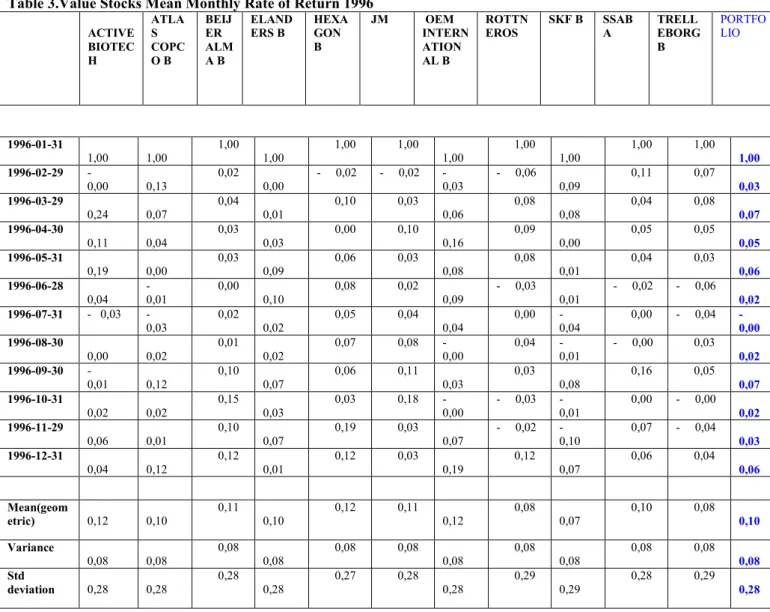
Table 3.Value Stocks Mean Monthly Rate of Return 1996 ACTIVE BIOTEC H ATLA S COPC O B BEIJ ER ALM A B ELAND
ERS B HEXAGON B JM OEM INTERN ATION AL B ROTTN
EROS SKF B SSABA TRELLEBORG
B PORTFO LIO 1996-01-31 1,00 1,00 1,00 1,00 1,00 1,00 1,00 1,00 1,00 1,00 1,00 1,00 1996-02-29 -0,00 0,13 0,02 0,00 - 0,02 - 0,02 -0,03 - 0,06 0,09 0,11 0,07 0,03 1996-03-29 0,24 0,07 0,04 0,01 0,10 0,03 0,06 0,08 0,08 0,04 0,08 0,07 1996-04-30 0,11 0,04 0,03 0,03 0,00 0,10 0,16 0,09 0,00 0,05 0,05 0,05 1996-05-31 0,19 0,00 0,03 0,09 0,06 0,03 0,08 0,08 0,01 0,04 0,03 0,06 1996-06-28 0,04 -0,01 0,00 0,10 0,08 0,02 0,09 - 0,03 0,01 - 0,02 - 0,06 0,02 1996-07-31 - 0,03 -0,03 0,02 0,02 0,05 0,04 0,04 0,00 -0,04 0,00 - 0,04 -0,00 1996-08-30 0,00 0,02 0,01 0,02 0,07 0,08 -0,00 0,04 -0,01 - 0,00 0,03 0,02 1996-09-30 -0,01 0,12 0,10 0,07 0,06 0,11 0,03 0,03 0,08 0,16 0,05 0,07 1996-10-31 0,02 0,02 0,15 0,03 0,03 0,18 -0,00 - 0,03 -0,01 0,00 - 0,00 0,02 1996-11-29 0,06 0,01 0,10 0,07 0,19 0,03 0,07 - 0,02 -0,10 0,07 - 0,04 0,03 1996-12-31 0,04 0,12 0,12 0,01 0,12 0,03 0,19 0,12 0,07 0,06 0,04 0,06 Mean(geom etric) 0,12 0,10 0,11 0,10 0,12 0,11 0,12 0,08 0,07 0,10 0,08 0,10 Variance 0,08 0,08 0,08 0,08 0,08 0,08 0,08 0,08 0,08 0,08 0,08 0,08 Std deviation 0,28 0,28 0,28 0,28 0,27 0,28 0,28 0,29 0,29 0,28 0,29 0,28
Source: Abadiga and Neibig
The results on Table 3 show the monthly Mean Price Rate of Returns for each stock in the portfolio that is calculated as follows.
t t t p p p 1 .
From these mean monthly price rate of returns, the annual geometric mean price rate of return is calculated for each portfolio during the year using Microsoft Excel tools for Geometric
mean calculations. For example, ={GEOMEAN(1+(C93:C104))-1} is used to calculate the 1996 Mean Annual Price Rate of Return for Atlas Copco stock.
The third measurement of returns (that is, following Holding Period Return, Mean Annual Price Rate of Returns) is the Risk-Adjusted Rate of Return (in this study the Sharpe ratio is used). To calculate this, first the price variability of each stock during the year is computed. To calculate the standard deviation, the same mean monthly rate of returns data are used for each stock in the portfolio during the year and Microsoft Excel formula for computing standard deviations is utilized. For example, = STDEV(C93:C104) is the Excel formula used to calculate the standard deviation of the mean monthly price rates of return for Atlas Copco stock during 1996.
Once the standard deviation (STDV) of each stock is calculated, the next variable needed for the calculation of the Risk-Adjusted Rate of Return is the Risk-Free Rate. The values for this variable are shown in Appendix G and thus the appropriate mean Risk-Free Rate is computed for the period under consideration. In this particular example, that is year 1996, it is 0.057045. Using the formula for Sharpe ratio explained under section 2.3.3 the following calculation is done for year 1996.
Risk-Adjusted Return= STDV te Riskfreera HPR = 0,278084 0,057045 -0,711844 = 2,354684
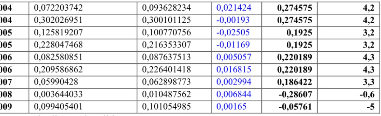
All these results are summarized in annual stock data tables that are attached as appendices B-F of which the data table for value Stock 1996 is reproduced here.
Table 12B. Value Stocks 1996
1996 VALUE STOCKS
COMAPNIES P/Ea DIVIDENDb STDc HPRd MEAN e
RETUR N ACTIVE BIOTECH 4,9 9,26 0,283175 1,430972 0,116014 ATLAS COPCO B 3,5 3,28 0,280852 0,874816 0,102039 BEIJER ALMA B 4,6 5 0,276457 1,256512 0,113277 ELANDERS B 6,1 1,81 0,279044 0,571648 0,098104 HEXAGON B 4,6 4 0,274425 1,685444 0,123626 JM ORD, 4,7 2 0,27727 0,971192 0,113321
Source: Abadiga and Neibig
What has so far been done is an illustration of how the three different measurements of returns are calculated.
3.5. Reliability
The term reliability means how trustworthy the data collecting methods, the use of data used and how it is processed.34 All data used in this study were taken from different independent
organizations (Börsguide by Delphi Economics, Thomas Reuters Ecowin Pro database and Central Statistical Bureau) where all data is presumed to be checked before they are published. We therefore believe there is no doubt regarding the reliability of the study.
Furthermore, we have chosen to apply well-tested models for calculations in order to minimize the risks of misleading and erroneous results and conclusions. However, there is always a risk of error. Looking at the large amount of data across various companies,
registered in the Swedish stock market, which is manually compiled from Börsguide and the amount of different calculations, there is a certain risk of error. Since we have been aware of this possibility, we have taken great care in compiling to minimize it.
3.6. Validity
Validity covers the relevance of data that is to represent the phenomenon under investigation and whether the study measures what it intends to measure.35 The data that we used in this
study is a prerequisite to answer the purpose and questions of this study. The study is based on historical data. The selected time period is important as the length of time assumed to
34 Johannessen, Asbjörn & Tufte, Per Arne, Introduktion till Samhällsvetenskaplig Metod, (Malmö: Liber 2003), uppl 1:2, p.28. 35 Ibid, p.47. OEM INTERNATIONAL B 6,1 2 0,278091 1,031042 0,118173 ROTTNEROS 2,5 0,2 0,287225 0,304184 0,082309 SKF B 5,9 5,25 0,289301 0,376594 0,074096 SSAB A 2,7 4 0,279999 0,810958 0,102705 TRELLEBORG B ORD, 3,3 3 0,286808 0,302688 0,076602 PORTFOLIO 0,278084 0,711844 0,097921 Rff 0,057045 SHARPEg 2,354684
include both the high and low performance periods for many stocks. This ensures accurate results across the various portfolios development over a given time period. The reference of this study is previously studies and how they have chosen to define value and growth stocks, the way they created different portfolios, what measures they have used and how they have arrived at their results.
3.7. Method Critic
During the formation of portfolios, stocks are grouped into value and growth categories using the highest and the lowest 30 % criteria through the help of Microsoft Excel filter tools. Each group is again ranked within itself according to its characteristics. For growth stocks, the ranking is made from the highest to the lowest with decreasing values while the value stocks were ranked from the lowest to the next lowest with increasing steps. Choosing twenty stocks from such a neat arrangement according to their rank in the group was the intention of this study. However, due to the absence of historical price data, particularly for the period 1996-1999 in Ecowin Pro, the study is forced to take only those stocks for which there are historical price data irrespective of where within the group ranking the stocks stand. This hampers the exactness of the results of the study. Added to this, the use of limited number of stocks in the first holding period (fourteen and eleven for growth and value stocks respectively) can have its own bias in the outcomes calculated.
The study of the characteristics of any stock market will not give an overall picture of the market without the study of the general behavioural characteristics of market participants. The dependence of this study on only quantitative study method deprives it of an additional tool in drawing a better conclusion. Method triangulation would have been a better approach for getting a better and closer observation of the market.