Henrik Andersson1,??, James Hammitt2, Gunnar Lindberg1, Kristian Sundstr¨om3
1 Dept. of Transport Economics, Swedish National Road and Transport Research Institute (VTI), Sweden 2 Center for Risk Analysis, Harvard University, USA
3 Swedish Institute for Food and Agricultural Economics (SLI), Sweden
July 3, 2008
Abstract Stated preference (SP) surveys attempt to obtain monetary values for non-market goods
that reflect individuals’ “true” preferences. Numerous empirical studies suggest that monetary values from SP studies are sensitive to survey design and so may not reflect respondents’ true preferences. This study examines the effect of time framing on respondents’ willingness to pay (WTP) for car safety. We explore how WTP per unit risk reduction depends on the time period over which respondents pay and face reduced risk. Using data from a Swedish contingent valuation survey, we find that WTP is sensitive to time framing; estimates based on an annual scenario are about 30 to 70 percent higher than estimates from a monthly scenario.
Key words Car safety, Contingent valuation, Double bound, Willingness to pay JEL codes C52; D6; I1; Q51
? Funding for this research was provided by VINNOVA. The authors are solely responsible for the results
presented and views expressed in this paper.
?? To whom correspondence should be addressed. Corresponding address:
1 Introduction
The monetary value of reducing road mortality risk is, together with the monetary value of reduced travel time, one of the dominating components of the benefit side in a benefit cost analysis (BCA) of transport investments and policies. This can explain the substantial literature on studies estimating the value of traffic safety (Andersson and Treich, 2008). The dominant approach to derive the value of safety is the willingness to pay (or willingness to accept) approach, where the tradeoff between risks and wealth is estimated. For mortality risks, this value is usually referred to as the value of a statistical life (VSL). Since the VSL measures how much wealth individuals are prepared to trade for small reductions in mortality risk, it is a measure of individuals’ preferences. To estimate VSL, since there are no easily available market prices for mortality risk reductions, analysts have to rely on non-market evaluation techniques. These techniques can, broadly speaking, be classified as revealed- or stated-preference (SP) techniques. The former refers to an approach where individuals’ market choices are used to derive the VSL. The hedonic regression technique (Rosen, 1974) has dominated this approach to estimate the VSL. It has mainly been used on the labor market where workers’ willingness to accept riskier jobs for larger monetary compensation has been estimated (Viscusi and Aldy, 2003). It has also been used in the car market to derive car consumers’ WTP for safer cars (Atkinson and Halvorsen, 1990; Dreyfus and Viscusi, 1995; Andersson, 2005, 2008).
The SP approach enables the analyst to tailor the survey/experiment to elicit preferences for spe-cific risks, even when no market exists (e.g., because of potential free riding (Carson and Hanemann, 2005)), and has been used in a large number of studies (Hammitt and Graham, 1999; Andersson and Treich, 2008). This flexibility is its major advantage compared to the RP approach. However, its major drawback is the hypothetical scenario itself, and the fact that respondents are often asked to state their preferences for goods that are unfamiliar and for which they have little experience. This unfamiliarity with the good could explain some of the evidence suggesting survey respondents do not have well-defined preferences. For instance, numerous empirical studies have found evidence of preference reversals as a result of variations of survey and experimental design (Tversky et al., 1990; Tversky and Thaler, 1990; Irwin et al., 1993). Similarly, some SP studies have found that respondents exhibit anchoring/starting-point bias, where their stated WTP is influenced by the bid levels presented in the survey (Herriges and Shogren, 1996; Boyle et al., 1997, 1998; Green et al., 1998; Roach et al., 2002). Results have also been found to be influenced by the amount of information given and the possibility of learning as part of the survey/experiment (Corso et al., 2001; Bateman et al., 2008). Other problems often raised in relation to SP studies are hypothetical and strategic bias, and in the case of eliciting preferences for risk changes a
lack of understanding of small probability changes (Andersson and Svensson, 2008; Bateman et al., 2002; Blumenschein et al., 2008).
The aim of this study is to estimate VSL for car safety. The main objective, beyond estimating values that can be considered for policy use, is to examine how VSL is related to the time frame presented to respondents. When considering their WTP for a good, survey respondents must consider the time frame, i.e., when and how often payments are to be made, and for how long the good will be provided. The objective of this study is to examine whether respondents’ rate of substitution between wealth and car safety is sensitive to the time framing of the scenario. This research question is of major policy relevance, and of general interest to the evaluation of non-market goods, since if the estimated rate of substitution is sensitive to the time frame, BCA will require values that are appropriate to the time frame relevant to a specific policy. If the sensitivity is too great, it suggests that SP methods may not measure a stable rate of substitution that is relevant to BCA.
To estimate VSL and study the effect of time framing, we conduct a contingent valuation (CVM) survey using a double-bounded dichotomous choice format (Hanemann et al., 1991) on a Swedish sample of ca. 900 individuals. It is not obvious which is the relevant time frame for different non-market goods, but often an annual scenario is used. We examine how stated WTP is affected by dividing our sample into two subsamples, presented with annual and monthly time frames, respectively. The scenarios are designed so that if the rate of substitution between wealth and current mortality risk is stable, the two time frames will yield similar estimates of VSL.
This is perhaps the first study that tests how time framing influences estimates in a CVM study. This is relevant to comparing results of studies that presented respondents with risk reductions over annual and longer periods. For example, some recent studies asked respondents whether they would purchase a safety product that would reduce their risk over a 10 year period, where payments were to be made annually (Krupnick et al., 2002, 2006; Alberini et al., 2004, 2006). In this study we show that a series of payments for risk reductions can be a good approximation for a single longer time period, and we examine empirically the effect of the time framing. Neither was done in the above mentioned studies. Moreover, Hammitt and Haninger (2007) asked respondents about their WTP for food safety where one subsample was asked about their WTP per portion and another sample about their WTP per month. Their results suggested that WTP per unit of risk reduction was not sensitive to the framing of the scenario. Our scenario differs from Hammitt and Haninger (2007) since they relate WTP for a specific time period to the quantity consumed during that time period.1
1 Beattie et al. (1998) asked respondents to state their WTP for a one year and a five year road safety program,
where the one and five year program was expected to prevent 15 and 75 lives, respectively. Thus, Beattie et al. (1998) confounded a test of scale sensitivity with time framing. Using an open-ended format, the WTP for the five
In the following sections 2, 3, and 4, we describe the VSL framework with its theoretical predictions, the survey administration and design, and the empirical models. We present our results in section 5 which suggest that VSL is sensitive to time framing, but that the difference in estimates is not too large compared with other uncertainties in estimating VSL. In addition, we show that policy values are sensitive to estimation approach used, non-parametric and parametric. Finally in section 6 we discuss our findings and draw some conclusions.
2 The theoretical framework
The VSL is the marginal rate of substitution (MRS) between risk and wealth (Jones-Lee, 1974; Rosen, 1988). Considering a standard single-period model, the individual is assumed to maximize his state-dependent indirect expected utility,
EU (w, p) = pud(w) + (1 − p)ua(w), (1)
where w, p, and us(w), s ∈ {a, d}, denote wealth, baseline probability of death, and the state dependent utilities, respectively, with subscripts a and d denoting survival and death. We adopt the standard assumptions that ua(w) and ud(w) are twice differentiable with
ua > ud, u0
a > u0d≥ 0, and u00s ≤ 0, (2)
i.e. us(w) is increasing and weakly concave, and ∀ w utility and marginal utility are larger if alive than dead. Totally differentiating Eq. (1) and keeping utility constant results in the standard expression for the MRS(w, p), VSL = dw dp ¯ ¯ ¯ ¯ EU constant = ua(w) − ud(w) pu0 d(w) + (1 − p)u0a(w) , (3)
where prime denotes first derivative. Under the properties of (2) VSL is positive, and increasing with w and p (Jones-Lee, 1974; Weinstein et al., 1980; Pratt and Zeckhauser, 1996).
Equation (3) denotes marginal WTP. In surveys respondents are asked about their WTP for a small but finite risk reduction, ∆p, and VSL is then the ratio between WTP and ∆p. The respondents’ WTP for ∆p is then approximated as,
W T P = VSL · ∆p, (4)
hence, WTP should be near-proportional to ∆p, a necessary (but not sufficient) condition for WTP from CVM-studies to be valid estimates of individuals’ preferences (Hammitt, 2000).2
year program was about twice the WTP of the one year program, hence scale sensitive but not near-proportional (Hammitt, 2000).
2 Equation (3) can be used to illustrate the effect on VSL from ∆p, which will be less than or equal to
Equation (4) defines the respondents’ WTP in a single-period model, e.g. a year. In this study we are interested in how respondents’ WTP is affected by how this time period is defined, i.e. the length of the time period. Since a longer time period can be seen as a series of shorter time periods, it also means that respondents’ WTP for a risk reduction during a longer time period can be redefined as a series of payments and risk reductions (∆pt). WTP at τ for a series of discrete risk reductions can be evaluated by, WTPτ = 1 (1 − pτ) T X t=τ ½ qτ,t (1 + i)t−τ ua(ct) u0 a(cτ)∆pt ¾ , (5)
where pτ is the probability of dying during period τ conditional on entering the period alive, qτ,t = (1 − pτ) . . . (1 − pt−1) is the probability at τ of surviving to period t, i is the utility discount rate, and ct is the optimal consumption level at t (Johansson, 2001, 2002; Morris and Hammitt, 2001).
In this study we examine how respondents’ WTP is affected by being presented with an annual or monthly risk reduction. Let WTPyτ denote the respondents’ WTP at τ for a one year ∆p, as given by Eq. (4). The monthly scenario is designed as a series of 12 identical risk reductions that sums up to the annual risk reduction, ∆p. Assume that optimal consumption is constant during the year, then Eq. (5) for the monthly scenario can be written as,
WTPmτ = ua(cτ) ∆p 12 ¡ 1 −pτ 12 ¢ u0 a(cτ) 12 X t=τ ½ qτ,t (1 + i)t−τ ¾ = " 1 − pτ 12¡1 − pτ 12 ¢ 12 X t=τ ½ qτ,t (1 + i)t−τ ¾# WTPyτ. (6)
For small p and i the expression within the brackets will be close to and strictly smaller than one. To illustrate, let the baseline risk be constant, e.g. p = 1/1000, and the monthly utility discount rate equal to zero, i.e. i = 0, then we have WTPm
τ = 0.999 · WTPyτ. The ratio between WTPmτ and WTPyτ depends on the size of p and i and the deviation from unity is increasing with both. For instance, letting i = 0.01 results in a ratio of 0.946 and and letting and p = 1/100 yields a ratio of 0.986. Hence, even with relatively large baseline risk levels and/or discount rates, the ratio is close to one.3
suggests that the income elasticity of VSL is between zero and one (Hammitt et al., 2006), evidence that can be used to show that the income effect will only cause a small departure from near-proportionality (Hammitt, 2000).
3 In appendix A the analysis is extended and we show that the difference between the single and multiperiod
3 Contingent valuation survey
3.1 Survey administration and design
The CVM survey was conducted in Sweden in the fall of 2006. Prior to the main survey the questionnaire was tested in focus groups and in a pilot.4 The main survey was distributed to 1,898 randomly chosen
individuals as a postal questionnaire. A total of 34 surveys could not be delivered because “recipient un-known” (e.g. the respondents had moved or the address was incorrect). Respondents who returned their questionnaire were awarded with a lottery ticket (nominal value of SEK 25), and after two reminders a 46.7 percent response rate was reached, i.e. n = 871.5 Respondents were also informed in the
accom-panying cover letter that they had the opportunity to complete the questionnaire on the web. Only 46 respondents chose that option, however, and in order to mitigate survey heterogeneity only the answers from the postal questionnaire are analyzed.6
In the main questionnaire all respondents were asked about their WTP for food and car safety. Bid and risk-reduction levels were randomly assigned, but all respondents were asked about WTP for food safety before WTP for car safety. The main questionnaire consisted of five sections, in the following order: (i) questions related to food, such as risk perception, handling, consumption, experience, etc., (ii) an evaluation example to train respondents in trading wealth for safety, (iii) WTP for food safety, (iv) WTP for car safety, and (v) follow-up questions on demographics and socio-economics. The effect of time framing was tested in the car safety scenario and so we report only results from the analysis of car safety. In the training section respondents were asked to choose between two goods, with one cheaper but with a higher baseline risk. Unlike some other studies, we did not include a dominant alternative and so cannot use this question as an exclusion criterion for probability comprehension (Krupnick et al., 2002; Alberini et al., 2004). Instead we used two other exclusion criteria based on an assumption of general survey comprehension. Respondents were excluded if they: (i) stated that their health status would be higher if they developed salmonellosis than if they did not, or (ii) gave inconsistent answers
4 The pilot, a postal questionnaire, was sent out to 202 randomly chosen individuals, out of whom 91 returned
completed questionnaires (44.1 percent response rate). The sample for the pilot was split into two groups; one received questions on food and car safety, the other only on food safety. The objective was to test if the survey length had a negative effect on the response rate. We did not find any evidence of that, in fact, the response rate was slightly higher in the group who had to answer the longer questionnaire, 45.4 against 42.9 percent. For a fuller description of the survey and the subgroups, see Sundstr¨om et al. (2008).
5 The lottery ticket had the effect that some empty questionnaires were returned, 103 in the main survey and
8 in the pilot. (Empty questionnaire not included in response rates reported here.) All prices are in 2006 price level. USD 1 = SEK 7.38 (www.riksbank.se, 2/11/2008)
6 Not including the respondents from the web survey only had minor qualitative effects on the results. See
to the double-bounded dichotomous-choice WTP questions for car safety. The latter was possible due to the postal format of the questionnaire.7
Respondents were informed in the training section that the social security system would cover any financial losses and medical expenditures due to illness and were reminded about their budget constraint. Hence, respondents’ WTP should reflect their WTP to reduce the risk of an adverse health effect ex-cluding financial consequences, which is parallel to the CVM scenarios in sections (iii) and (iv) of the questionnaire. After their decision, respondents were given feedback and once again reminded of the coverage of the social security system and their budget constraint.
To communicate the risks, respondents were provided with a visual aid in the form of a grid consisting of 10,000 white squares with the risks visualized as black squares in the training session and in the section on WTP for food safety. Previous research suggests that this form of visual aid can improve respondents’ understanding of the risk/money tradeoffs (Corso et al., 2001). Since the visual aid had been presented twice to the respondents before the WTP scenario on car safety, we decided that it was not necessary to include it in that section.
3.2 Willingness to pay for car safety
Before answering the question on WTP for car safety, respondents were provided with some background questions related to driving and travelling by car (driving license, access to a car, “driving distance”, injury experience, and risk perception). We had two objectives with these questions: (i) to gather infor-mation that could be used in the analysis, and (ii) to act as a “warm up” for the new scenario, i.e. we wanted to make sure that respondents were thinking about car and not food safety when answering the WTP question.
The respondents were split into two subsamples, one received a monthly scenario and the other an annual scenario. In each scenario both risks and payments were adapted to time frame given. Respondents in the monthly and annual scenario were informed that the objective risk was 6 per 1,000,000 and 7 per 100,000, respectively. The design of the monthly scenario was such that if a respondent was prepared to pay for the safety device during a whole year, i.e. twelve identical payments, his risk reduction and payment would be equal to the annual scenario. Small adjustments were be made to yield integer values and discount factors are assumed negligible and neglected.
The safety device was described as an abstract device (Jones-Lee et al., 1985) that the respondents had the opportunity to rent for a specific time period (a year or a month, depending on which subsample 7 Due to the postal format we could not control how the respondents answered the survey. It was, therefore,
possible for respondents to answer the wrong follow-up questions (e.g. answering the follow-up question to an initial no-answer, after stating that they were willing to pay the initial bid).
they belonged to). Respondents were told that they had to pay a lump sum and that they had the opportunity to extend the rental period, but that they then had to pay the lump sum again. The device was described as follows (freely translated from Swedish):
“You rent the safety device for a period of one [year], for which you pay a lump sum. If you want to continue using the device after one [year] you may extend the rental period, but then you have to pay anew. The safety device will only reduce the risk of dying, not the risk of being injured. The device only protects yourself and not any other passengers. The device will not affect the car’s characteristics in terms of appearance, comfort or driving characteristics.”
Prior to the WTP question, respondents were asked about their perception on their own risk of dying as a result of a car crash. The baseline risk was randomly assigned (not based on the respondent’s own perceived risk), though. We assigned one of two initial and two final risk levels, which resulted in three risk reductions. Final risks were always positive to avoid a potential certainty premium from risk elimination (Kahneman and Tversky, 1979; Viscusi, 1998). By varying both the initial and the final risk levels, we obtained risk reductions of different magnitude such that absolute and proportional risk reductions are not perfectly correlated. Risk levels were close to the average objective risk (i.e., 7 per 100,000 per year) to increase realism. The initial risk levels without the safety device were slightly larger, and those with the device they were slightly smaller, than the average objective risk. Risk and bid levels are summarized in Table 1.
[Table 1 about here.]
The bid levels in Table 1 are the initial bid levels. Follow-up bids for the double-bounded format are twice as large as the initial bid for respondents who answered yes to the initial bid, and half as large as the initial bid for respondents who answered no. We also calculate single-bounded estimate based only on respondents’ answers to the first question.
4 Empirical models
This section briefly describes the econometric models and specifications used. We first describe the non-parametric estimation used to estimate preferred policy values and then the parametric models for validity testing and potential use in benefit transfers.8
8 Since we use standard and well known estimation techniques, this section has been kept to a minimum. For
readers interested in more detailed descriptions of the models and techniques we recommend, e.g., Bateman et al. (2002) or Haab and McConnell (2003).
4.1 Non-parametric estimation
Non-parametric estimation offers an advantage over parametric estimation since it does not rely on distributional assumptions made by the analyst. In this study we use Turnbull’s lower bound (TB) estimator of WTP (Turnbull, 1976).9As a lower bound, TB is a conservative estimate of WTP and of VSL
that protects against the tendency for respondents in SP studies to overstate their WTP (Blumenschein et al., 2008), usually referred to as hypothetical bias. A drawback of using the TB is that it will not necessary be proportional to the size of the risk reduction, even if WTP is proportional. Hence, when using TB we cannot use proportionality of WTP to risk reduction as a validity test.
Let bj and F (bj) denote the bid and the the proportion of no answers to the offered bid. The TB mean WTP is estimated by ET B[W T P ] = J X j=0 bj(F (bj+1) − F (bj)) , (7)
where it is assumed that F (0) = 0 and F (∞) = 1, i.e. no respondent has a negative or infinitive WTP, and that F (bj) is weakly monotonically increasing. When F (bj) is non-monotonic, the pooled adjustment violators algorithm (PAVA) needs to be used prior to estimation of Eq. (7) (Turnbull, 1976; Ayer et al., 1955). Equation. (7) can be used for interval data when bid ranges are non-overlapping. The bid levels in our DB scenario result in bid ranges that are overlapping, however. We, therefore, have to use Turnbull’s self consistency algorithm (TSCA). The TSCA divide the bids into “basic intervals” and allocate observations to each interval through an iteration process until the survival function converges (Bateman et al., 2002, pp. 232-237).10
4.2 Parametric estimation
The main purpose of the parametric estimation is to examine how different covariates influence WTP, not to examine the underlying structural model. Since the coefficient estimates of the bid-function approach show the marginal impact on WTP of different covariates (Cameron and James, 1987; Cameron, 1988; Patterson and Duffield, 1991; Cameron, 1991; Bateman et al., 2002), our parametric models are based on the bid-function approach (instead of the utility-function approach Hanemann (1984)).
We assume a multiplicative model. Taking logs results in the econometric model estimated,
ln(W T Pi) = α + β1ln(∆pi) + K X k=2
βkfk−1(xi) + εi, (8)
9 The Turnbull lower bound estimator is also known as the Kaplan-Meier estimator (Carson and Hanemann,
2005).
where f (x) defines dummy variables and the natural logarithm of continuous variables. Proportionality between WTP and ∆p require that β1= 1. Preliminary analysis showed that a normal distribution fits
our data best, and we therefore estimate a log-normal model (Alberini, 1995a). The log-normal model rules out the possibility of zero WTP and to allow for respondents’ WTP being equal to zero, Eq. (8) is estimated as a mixture model (An and Ayala, 1996; Haab, 1999; Werner, 1999). To estimate the mixture model we use the answers from a follow-up question to respondents who answered “no-no” which allow us to identify those respondents whose WTP equals zero. The mixture model is our preferred parametric model, but we also report regression results for the conventional log-normal model.11
We follow the recommendation of Bateman et al. (2002, p. 243) and omit the covariates of Eq. (8) to estimate the unconditional mean and median WTP of our sample. However, to examine scale sensitivity and time framing it is necessary to control for these variables. Thus, in addition to the constant, our estimate of WTP is based on parametric models which include a continuous variable for the risk change, ∆p, and a dummy for the time frame scenario, Year. Moreover, since the median is a more robust measure of central tendency we estimate median instead of mean VSL, and due to the non-normality of the WTP distribution our confidence intervals for median VSL are estimated using bootstrapping (Bateman et al., 2002; Haab and McConnell, 2003).
5 Results
5.1 Descriptive statistics
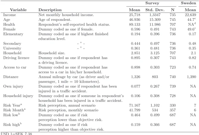
The descriptive statistics are shown in Table 2. Our sample appears to be representative of the general Swedish population of the relevant age group (18-74). The exceptions are the proportion of female respondents, which is higher compared with the general population, 59.6 vs. 49.6 percent, and larger household size in the sample compared with the general population. One reason for the high share of female respondents could be because the first half of the survey concerned food risks and Swedish women are responsible for most of the household food production (> 60%) (Rydenstam, 2008).
The respondents reported a slightly lower annual distance traveling by car, 1,326 compared with 1,390 Swedish miles (1 mile = 10 kilometers), even if the share of respondents with a driving license and access to a car in the household was higher than the general population. Regarding injury experience it is hard to relate the number from the survey with objective data. Statistics on reported injuries from road accidents reveal an annual objective risk equal to 0.3 percent, which is considerably smaller than the 7.7 and 10.6 percent stated by the respondents. However, respondents were asked whether they or anyone 11 For readers not familiar with the mixture model, see appendix B for a brief description of the difference
in their household had ever been injured as a result of a road accident. Moreover, official statistics are likely to underestimate actual injury risk since not all injuries are reported. Further, individuals with injury experience may have more interest in completing a questionnaire related to road safety.
Respondents were asked to state how they perceived their own health status and mortality risk in road traffic. To obtain self-reported health status we used a visual analog scale in the form of a ther-mometer ranging from 0 to 100, where 100 is the best imaginable health state. Mean self-reported health was slightly higher than previous Swedish estimates (Brooks et al., 1991; Andersson, 2007; Koltowska-H¨aggstr¨om et al., 2007). Regarding perceived mortality risk, more respondents stated that their own risk was lower than the average objective risk. However, due to a small number of large values, estimated arithmetic perceived means are higher than the objective risk.
[Table 2 about here.]
5.2 WTP distribution and non-parametric analysis
The distribution of yes answers to the WTP questions together with the non-parametric estimates of WTP are shown in Table 3. Focusing on the respondents’ answers to the initial bid (SB), the results reveal that the proportion of yes answers is uniformly decreasing for only half of the subsamples. For those that are not, the PAVA was used prior to the estimation of WTP (Turnbull, 1976; Ayer et al., 1955). Kanninen (1995) showed that bids that covered the center of the WTP distribution were most efficient for obtaining efficient estimates of mean and median WTP. As a rule of thumb, Kanninen suggested that bids should be limited to be within the 15th and 85th, and 10th and 90th, percentiles of the WTP distribution for SB and DB models, respectively. For the SB answers we find that the share of respondents accepting the lowest bid is higher than 85 percent in only one subsample, and the share of respondents accepting the highest bid is lower than 15 percent in all but one subsample. The distribution of the DB answers reveals a similar pattern with only one subsample having a share of respondents accepting the lowest bid higher than 90 percent, and with no subsample having a share of respondents accepting the highest bid higher than 10 percent.
[Table 3 about here.]
Estimated mean WTP reveals mixed results. In the annual and monthly SB models, WTP is, as expected, lowest for the smallest risk reduction. In the monthly scenario we also find that the highest WTP is for the largest risk reduction. In the annual scenario, however, the highest WTP is found for the intermediate risk reduction. The DB models reveal the same pattern for WTP in the annual scenario, i.e. the lowest and highest WTP for the smallest and the intermediate risk reduction, respectively.
However, in the monthly scenario we find a WTP that is monotonically decreasing with the size of the risk reduction. Regarding the effect from time framing, we find no such effect for ∆p = 4, some effect for ∆p = 8, and a considerable effect in the SB model for ∆p = 6.
5.3 Parametric analysis
The regression results from the parametric analysis are shown in Tables 4 and 5. To test the robustness of our results, we: (i) run regressions including all respondents (conditional on the exclusion criteria in section 3), and (ii) including only those respondents who in a follow-up question did not state that they found the scenario unrealistic. Since we included a qualitative question on preference certainty (completely or rather certain), an alternative would have been to run the regressions based on certainty calibration (Blumenschein et al., 2008). However, the results based on certainty calibration depend on how we treat uncertain answers; a symmetric exclusion criterion would reveal similar estimates to the ones presented, whereas an asymmetric criterion, where only yes answers were treated as certain or uncertain, would reveal a lower WTP.12 To examine the effect of using the mixture model, we also run
conventional log-normal regressions, where the WTP is strictly positive.
The results from the regressions with only ∆p and Year as explanatory variables are shown in Table 4. We find that the estimated coefficient for ∆p is statistically insignificant in all regressions. The same result was found when ∆p was replaced by dummy variables for each size of the risk reduction. The results also suggest that not allowing WTP to be equal to zero results in weaker scale sensitivity in our sample. The coefficient for Year is not statistically significant in any of the regressions of the mixture model. It is positive and statistically significant in the conventional DB model. The coefficient estimate of this model suggests that WTP in the annual scenario is 43 percent higher than in the monthly scenario.13,14
[Table 4 about here.]
12 Using monthly WTP with ∆p = 4 as the reference, the symmetric certainty calibration results in slightly
higher and lower WTP with one exception. WTP from the “DB - All respondents”, is about one third lower than the estimate in Table 6. The asymmetric certainty calibration results in values that are 20 to 40 percent lower than the values for monthly WTP with ∆p = 4 in Table 6. The “certainty calibration” regressions in general reveal a stronger scale sensitivity than the regressions shown in Tables 4 and 5. This is especially true for the symmetric criterion where the coefficient estimates, with one exception, are in the interval 0.60 to 0.96. The coefficients are still not statistically significantly different from zero, though.
13 e0.356− 1 = 0.43
14 A validity test of CVM studies with dichotomous choice questions is that the coefficient of the bid is negative
and statistically significant, i.e. respondents should be less likely to accept the bid when the bid is higher. Regression with the bid and the same covariates as in Tables 4 and 5 on the probability of accepting the bid showed that the bid coefficient was negative and highly significant (p < 0.01) in all regressions. Moreover, to test whether respondents’ answers to the initial and follow-up bid were from the same WTP distribution, bivariate probit regressions were run (Alberini, 1995b). The results showed that the correlation between the errors was high (ca. 0.8) statistically significantly different from zero (p-value < 0.01) and that the null hypothesis of identical coefficients could not be rejected (p-value > 0.8).
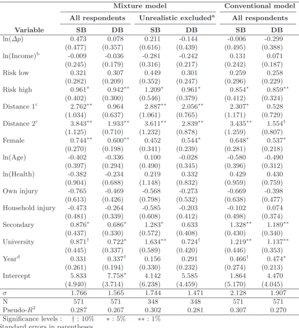
The results from the regressions including socio-economic and demographic variables are shown in Table 5. Again we do not find any significant relationship between WTP and ∆p. We also do not find the predicted positive relationship between WTP and household income, where Income is measured as income per consumption unit, i.e. household income divided by the weighted sum of household members based on age. Age, Health, and injury experience (own and household) are not statistically significantly correlated with WTP.
[Table 5 about here.]
Regarding risk perception, we find that respondents who perceive their own risk to be higher than the average objective risk have a significantly higher WTP than the reference group (perceived risk equal to objective risk). This significant correlation suggests that respondents may base their decision to accept the bid on their own perceived baseline risk, instead of the baseline risk given in the questionnaire. For the group that perceived its risk level to be lower than the objective risk, no significant correlation is found. We also find that those who drive or travel by car have a higher WTP than those who do not, that respondents who have attended only elementary school have a lower WTP than those with more education, and results that suggest that females have a higher WTP than men. Finally, Year is positive in all regressions, but statistically significant in only one of the mixture model regressions, i.e. DB including all respondents.15
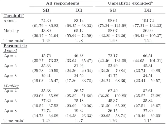
Estimated median WTP based on the regression results in Table 4 together with the confidence intervals are reported in Table 6. Monthly WTP was converted to annual WTP prior to the regression analysis and for ease of comparison, all WTP values are shown as annual WTP. The results in Table 6 show three patterns: (i) annual is higher than monthly WTP, 15 to 29 percent (ii) WTP is not proportional to the size of ∆p, and (iii) excluding respondents who regarded the scenario as unrealistic increases the WTP by 40 to 80 percent. This indicates that those who found the scenario unrealistic were more likely to reject the bid. Table 6 also reveals that DB WTP is in most cases lower than SB WTP, about 10 to 20 percent, a difference that is not statistically significant in any case.
[Table 6 about here.]
5.4 Estimates of the value of a statistical life
Our estimates of VSL from the non-parametric and parametric analyses are shown in Table 7. Again, the parametric estimates are based on results from the mixture models in Table 4. From the non-parametric 15 Including the respondents from the web questionnaire resulted in: (i) a weaker relationship between education
level and WTP with Secondary and University only statistically significant in “DB All respondents”, and (ii) that Year in “DB All respondents” became statistically insignificant.
analysis we report the weighted average for the SB and DB models conditional on the time frame. Our Turnbull VSL estimates reveal that the effect of time framing is highest in the SB models, 69 percent compared with 20 to 28 percent in the DB models. For the parametric estimates, the insensitivity to scale found in Tables 4 and 6 is reflected in the variation between estimates for different ∆p.
[Table 7 about here.]
6 Discussion
In this study we have estimated Swedish respondents’ WTP for car safety and examined how the time frame presented to them influences the results. Data from a Swedish dichotomous DB CVM study was used.
We find that estimated WTP and VSL are sensitive to the time framing of the question. Hence, in empirical applications it may be problematic to treat a one period risk reduction as equivalent to a series of risk reductions (Krupnick et al., 2002; Alberini et al., 2004). In the non-parametric analysis, estimates of the weighted average VSL based on the SB and DB formats were 69 and 28 percent higher in the annual than the monthly scenario. However, only the SB estimates were statistically significantly different. In the parametric analysis the results were mixed, with one of the regressions of the mixture models suggesting that WTP in the annual scenario was ca. 40 percent higher than in the monthly scenario, but with the other regressions finding no statistically significant relationship. Overall, we conclude that our results suggest that preference elicitation for car safety is sensitive to time framing, but that the problem is modest in comparison with other aspects of preference elicitation for mortality risk reductions, i.e. especially scale insensitivity.
The fact that the estimated VSL from the annual scenario is higher than the estimates from the monthly scenario is in line with our expectations. However, based on Eq. (6) in section 2 which showed that VSL should be close to identical under reasonable assumptions, the difference is larger than expected. One plausible explanation, which would suggest that the monthly scenario may be preferred to the annual in SP studies, is that respondents might have found the monthly scenario easier to evaluate. Wages and salaries are often received on a monthly basis and many expenditures are paid monthly, e.g. rent and telephone bills. Thus, it may be easier to relate the cost to the budget constraint in the monthly scenario, and the lower estimates might, therefore, reflect less yes-saying and hypothetical bias (Boyle et al., 1998; Blumenschein et al., 2008). It could also have been the case that respondents were more reluctant to accept the amount offered in the monthly scenario due to the small risk reduction (per million compared with per 100,000 in the annual scenario). However, if the respondents were influenced by the risk reduction and bid levels, the effect of the former would have been offset by the effect of
the latter, with the combined effect being indeterminate. Hence, any explanation about the difference is only speculative, but the results highlight the importance of the time frame chosen by the analyst when estimating WTP.16
Estimates were found to be robust between SB and DB. In the parametric analysis, VSL estimates were close and not statistically significantly different, whereas the DB estimates from the non-parametric estimates were higher than the SB estimates. The DB format has raised concern since it might induce respondents to anchor their WTP on the initial bid, hence, the WTP distribution in the SB and DB regressions might not be identical. After having been presented with an initial cost (the bid) for the good, the second valuation question might come as something of a surprise to the respondent, as in surveys conducted in-person, or over the phone or the web. Depending on how the respondent perceives the new information he can be inclined to reject the follow-up bid, if he sees the new bid as a attempt of bargaining or cost overrun, or to accept the follow-up bid, if he wants to show commitment after an initial yes-answer or feels “guilty” after rejecting the initial bid and should pay at least the lower amount (Hanemann and Kanninen, 1999). We avoid this element of surprise since we use the postal format in which respondents know that there will be a follow-up bid.
We found that estimated WTP was sensitive to how observations from respondents who did not consider the scenario realistic were treated. Excluding these respondents resulted in estimates that were 40 to 80 percent higher than the values when all respondents were included. This result suggests that respondents who do not believe in the hypothetical scenario are more likely to reject the bid offered to them. The policy implications of this finding is unclear, however. On one hand, values based on a sample including respondents who did not believe in the hypothetical scenario and therefore rejected the bid can be considered to be biased downward. On the other hand, faced with the same decision in a real life situation, the respondent would not pay for the good or vote for the safety measure in a referendum, which means that excluding these respondents may result in a positive bias of the population WTP.
We do not find the expected positive relationships between WTP and the size of the risk reduction and income level in our parametric analysis. On the other hand, we cannot reject proportionality in every regression. Whereas near-proportionality is usually rejected in the empirical literature, WTP is often found to be scale sensitive and positively related to income, even though similar findings to ours are not uncommon (Hammitt and Graham, 1999; Andersson and Treich, 2008). The results from the
non-16 The distribution of respondents who found the scenario realistic was nearly identical between the annual and
parametric analysis are mixed. The results from several subgroups suggest that WTP is scale sensitive, with some estimates also suggesting near-proportionality.17
It seems intuitive that age and health status should be negatively and positively related to WTP, respectively. However, the theoretical predictions for age and health status are indeterminate (Johansson, 2002; Hammitt, 2002). Our findings that age and health status are not correlated with WTP is consistent with other empirical results in the CVM literature (Krupnick, 2007; Alberini et al., 2004, 2006; Andersson, 2007). Regarding other covariates, we find that WTP is higher among respondents who drive or travel by car and have more education. The insignificant relationship between WTP and Income but significant relationship between WTP and schooling suggests that schooling may be a better proxy for wealth than income. Moreover, whereas other Swedish studies using the CVM have not found a statistically significant relationship between gender and WTP to reduce transport related mortality risk (Johannesson et al., 1996; Hultkrantz et al., 2006; Andersson, 2007), we find that women are willing to pay more than men.18
Our preferred values are the ones from the non-parametric models. The values for the full samples are in the range SEK 43.86 to 83.14 million, depending on time frame and whether based on SB or DB. These values are considerably higher than the official VSL in use in Sweden, SEK 17.31 million (SIKA, 2005), which is based on the results from a CVM study (Persson and Cedervall, 1991).19 The range is
also considerably higher than the findings in Persson et al. (2001), SEK 24.70 million. However, when analyzing the same data as Persson et al., Andersson (2007) estimated VSL to be in the range SEK 28.20 to 142.96 million, the wide range being a consequence of model assumptions and the rejection of near-proportionality. For a risk reduction in the form of a private good, Hultkrantz et al. (2006) and Johannesson et al. (1996) estimated VSL to be 53.95 and 49.41 million, values that are within the range of our estimates.20
Appendix
A Multiperiod models and a background risk
The life-cycle period model has been used to predict how WTP varies with age, and it can be shown that WTP over the life cycle will depend on the optimal consumption path (Shepard and Zeckhauser, 17 Some recent studies have shown that with: (i) a better understanding among analysts of why WTP in CVM
study fails the validity tests, and (ii) improved survey design improving respondents’ understanding of the scenario (e.g. by training or visual aids), WTP can be scale sensitive in line with the theoretical predictions (Hammitt and Graham, 1999; Corso et al., 2001; Alberini et al., 2004; Andersson and Svensson, 2008).
18 Johannesson et al. (1996) found that WTP was statistically significantly higher among females for a public
good, but not for a private good.
19 All values adjusted to 2006 price level using CPI (www.scb.se, 3/31/08) in this paragraph, including the
official VSL.
1984; Johansson, 2002). In the life-cycle model an individual’s expected utility is given by EUτ = ∞ X t=τ qτ,t(1 + i)τ −tu(c∗ t), (9)
where qτ,t= (1 − pτ) . . . (1 − pt−1) is the probability at t = τ of surviving to period t, i is the subjective rate of time preferences, and c∗
t is the optimal consumption level at t. Johansson (2002) showed that the optimal consumption path will depend on the assumptions of the model and that the effect of age on WTP is indeterminate. In this study we do not examine how WTP varies with age. Instead we use the life cycle model to examine how WTP per unit of risk reduction is affected by the time framing of the scenario. In addition, we extend our model and show how time framing influences our results when we have a background risk that is age-dependent.
We examine how an individual’s WTP at t = τ differs between a risk reduction that lasts over the interval [τ, τ + T ] and a series of risk reductions over T intervals. The length of the intervals and the size of T is no larger than we can assume that the optimal consumption path is constant during the interval, thus c∗
t = cτ. For instance, in our numerical example below our time intervals last a month and T = 12. The WTP for for the risk reduction that lasts over [τ, τ + T ] is defined as follows,
WTPsτ=
ua(cτ)
(1 − T pτ)u0a(cτ)T ∆pτ, (10)
which is our single period model (equivalent to Eq. (3) with no bequest motives, i.e. ud = 0), and the WTP for a series of T risk reductions as,
WTPmτ = 1 (1 − pτ) T X t=τ ½ qτ,t (1 + i)t−τ ua(ct) u0 a(cτ)∆pt ¾ . (11)
We follow the assumption of section 2 that ∆p is constant, which means the aggregated risk reductions in Eqs. (10) and (11) are the same. Based on our assumptions, Eq. (11) can be written as follows,
WTPmτ = " 1 − T pτ T (1 − pτ) T X t=τ qτ,t (1 + i)t−τ # | {z } Γ (T ) WTPsτ, (12)
where it can be shown that Γ (T ) < 1 and, ceteris paribus, decreasing with T . Hence, the multiperiod model will result in a WTP per unit of risk reduction that is strictly less than the single period model. The result that the multiperiod model will yield a lower bound WTP of the single period model is identical to the findings of Johannesson et al. (1997) when they examined the relationship between WTP for a blip and a permanent change of the hazard rate, i.e. they concluded that the WTP for the blip yields a lower bound for a permanent change.
So far we have assumed one aggregated measure of the baseline risk, p. We now extend our model and assume that the baseline mortality risk can be separated into a specific risk (r) and an aggregated
measure of other mortality risks that is allowed to depend on the age of the respondent (π(t)). These risks can be either multiplicative (Eeckhoudt and Hammitt, 2001) or additive (Evans and Smith, 2006; Andersson, 2008). We assume that the risks are multiplicative, r is constant, and ˙π(t) > 0, i.e. the background risk is increasing with age. The single period survival probability is then (1 − r)(1 − π(t)). It is straightforward that if π(t) is constant and the survival probability is the same in Eqs. (12) and (13), then the background risk will not affect Γ (T ),
By differentiating Γ (T ) in Eq. (12) w.r.t. t we can examine how the effect of time framing will be influenced by a background risk that is increasing with age. Let λ = 1 − r, then
∂Γ (T ) ∂t = − 1 − T pτ T (1 − pτ) T X t=τ +1 λt−τ˙q τ,t (1 + i)t−τ, (13)
where ˙qτ,t> 0, since πt< 1 and ˙π(t) > 0. Thus, a background risk that is increasing with age will reduce the size of Γ (T ) and increase the effect of time framing. The effect will be the largest when i = 0.
We will use a numerical example to illustrate the effect. Let π(t) = a exp(bt), where a = 0.000081 and b = 0.087 (Johannesson et al., 1997), and r = 1/10, 000 ⇒ λ = 0.9999. Since the effect will be the largest when the discount rate is zero, we also assume that i = 0. For a series of 12 monthly risk reductions we can show that the effect on an average 40 year old (for whom the annual mortality risk is 0.003) will be negligible, and that the effect for an average 70 year old (with annual mortality risk 0.036) will also be small, ∂Γ (12)40 ∂t = −0.0013, ∂Γ (12)70 ∂t = −0.0138. (14)
From Eq. (14) we conclude, when allowing for a background risk that is increasing with age, that the effect of time framing will increase with the age of the examined population However, Eq. (14) shows that also for older age groups, the effect of time framing will be small.
B The mixture model
When assuming a log-normal distribution, WTP equal to zero is ruled out. Incorporating zero WTP can be done by employing the mixture model (An and Ayala, 1996; Haab, 1999; Werner, 1999). This section briefly describes the difference between the DB conventional (WTP> 0) and mixture model. For a more detailed description of the mixture model see, e.g., An and Ayala (1996).
Let i = 1, ..., N , bi, bL
i and bHi , denote the index for each respondent, the initial bid, and the follow-up bids, respectively, with the sfollow-uperscripts referring to lower (L) and higher (H) follow-follow-up bids. The
respondents’ answers in a DB CVM are represented by the following four indicator variables:
D1i= 1 iff WTPi < bLi (“no-no” response) D2i= 1 iff bLi ≤ WTPi< bi (“no-yes” response) D3i= 1 iff bi≤ WTPi< bHi (“yes-no” response) D4i= 1 iff bHi ≤ WTPi (“yes-yes” response)
(15)
Let F (x; θ) denote the cumulative distribution function (CDF) for x with parameters θ, and our sample log-likelihood for the conventional model is then,
l(θ) = N X i=1 {D1iln[F (bLi; θ)] + D2iln[F (bi; θ) − F (bLi; θ)] + D3iln[F (bHi ; θ) − F (bi; θ)] + D4iln[1 − F (bHi ; θ)]}. (16)
Now, assuming that x ≥ 0, the CDF of x in the mixture model will have the form,
G(x; ρ, θ) = ½
ρ if x = 0
ρ + (1 − ρ)F (x; θ) if x > 0 (17)
i.e. G(x; ρ, θ) has a point mass ρ at x = 0.
The estimation of the mixture model depends on whether the analyst has information about which respondents that have a WTP equal to zero, information that can be obtained by asking a follow-up question to the “no-no” respondents. When this information is not available, ρ needs to be estimated and the log-likelihood is specified as follows,
l1(ρ, θ) = N X i=1 {D1iln[ρ + (1 − ρ)F (bLi; θ)] + D2iln[(1 − ρ)(F (bi; θ) − F (bLi; θ))] + D3iln[(1 − ρ)(F (bHi ; θ) − F (bi; θ))] + D4iln[(1 − ρ)(1 − F (bHi ; θ))]}. (18)
When xi = 0 is known to the analyst, ρ = N0/N , where N0 is the number of respondents with a
WTP equal to zero. For the log-likelihood we then need to introduce a new indicator variable, D0i, which
is equal to 1 if WTP is equal to zero. The log-likelihood with full information is then specified by
l2(ρ, θ) = N X i=1 {D0iln[ρ] + (D1i− D0i) ln[(1 − ρ)F (biL; θ)] + D2iln[(1 − ρ)(F (bi; θ) − F (bLi; θ))] + D3iln[(1 − ρ)(F (bHi ; θ) − F (bi; θ))] + D4iln[(1 − ρ)(1 − F (bHi ; θ))]} (19)
References
Alberini, A., M. Cropper, A. Krupnick, and N. B. Simon: 2004, ‘Does the Value of a Statistical Life Vary With the Age and Health Status?: Evidence from the USA and Canada’. Journal of Environmental Economics and Management 48(1), 769–792.
Alberini, A., A. Hunt, and A. Markandya: 2006, ‘Willingness to Pay to Reduce Mortality Risks: Evidence from a Three-Country Contingent Valuation Study’. Environmental and Resource Economics 33(2), 251–264.
Alberini, A.: 1995a, ‘Efficiency vs Bias of Willingness-to-Pay Estimates: Bivaraite and Interval-Data Models’. Journal of Environmental Economics and Management 29, 169–180.
Alberini, A.: 1995b, ‘Optimal Designs for Discrete Choice Contingent Valuation Surveys: Single-Bound, Double-Bound, and Bivariate Models’. Journal of Environmental Economics and Management 28, 287–306.
Andersson, H. and M. Svensson: 2008, ‘Cognitive Ability and Scale Bias in the Contingent Valuation Method’. Environmental and Resource Economics 39(4), 481–495.
Andersson, H. and N. Treich: 2008, Handbook in Transport Economics, Chapt. The Value of a Statistical Life. Edward Elgar, Forthcoming.
Andersson, H.: 2005, ‘The Value of Safety as Revealed in the Swedish Car Market: An Application of the Hedonic Pricing Approach’. Journal of Risk and Uncertainty 30(3), 211–239.
Andersson, H.: 2007, ‘Willingness to Pay for Road Safety and Estimates of the Risk of Death: Evidence from a Swedish Contingent Valuation Study’. Accident Analysis and Prevention 39(4), 853–865. Andersson, H.: 2008, ‘Willingness to Pay for Car Safety: Evidence from Sweden’. Environmental and
Resource Economics Forthcoming.
An, Y. and R. A. Ayala: 1996, ‘A Mixture Model of Willingness to Pay Distributions’. Mimeo, Duke University, USA, and Central Bank, Ecuador.
Atkinson, S. E. and R. Halvorsen: 1990, ‘The Valuation of Risks to Life: Evidence from the Market for Automobiles’. Review of Economics and Statistics 72(1), 133–136.
Ayer, M., H. D. Brunk, G. M. Ewing, W. T. Reid, and E. Silverman: 1955, ‘An Empirical Distribution Function for Sampling with Incomplete Information’. Annals of Mathematical Statistics 26(4), 641– 647.
Bateman, I. J., D. Burgess, W. G. Hutchinson, and D. I. Matthews: 2008, ‘Learning design contingent valuation (LDCV): NOAA guidelines, preference learning and coherent arbitrariness’. Journal of Environmental Economics and Management 55, 127–141.
Bateman, I. J., R. T. Carson, B. Day, M. Hanemann, N. Hanley, T. Hett, M. Jones-Lee, G. Loomes, S. Mourato, ¨Ozdemiro¯glu, D. W. Pearce, R. Sugden, and J. Swanson: 2002, Economic Valuation with Stated Preference Techniques: A Manual. Cheltenham, UK: Edward Elgar.
Beattie, J., J. Covey, P. Dolan, L. Hopkins, M. W. Jones-Lee, G. Loomes, N. Pidgeon, A. Robinson, and A. Spencer: 1998, ‘On the Contingnent Valuation of Safety and the Safety of Contingent Valuation: Part 1 - Caveat Investigator’. Journal of Risk and Uncertainty 17(1), 5–25.
Blumenschein, K., G. C. Blomquist, M. Johannesson, N. Horn, and P. Freeman: 2008, ‘Eliciting Willing-ness to Pay without Bias: Evidence from a Field Experiment’. Economic Journal 118(525), 114–137. Boyle, K. J., F. R. Johnson, and D. W. McCollum: 1997, ‘Anchoirng and Adjustment in single-Bounded,
Contingnent Valuation Questions’. American Journal of Agricultural Economics 79(5), 1495–1500. Boyle, K. J., H. F. MacDonald, H. Cheng, and D. W. McCollum: 1998, ‘Bid Design and Yes Saying in
Single-Bpunded, Dichotous-Choice Questions’. Land Economics 74(1), 49–64.
Brooks, R. G., S. Jendteg, B. Lindgren, U. Persson, and S. Bj¨ork: 1991, ‘EuroQol: Health-Realted Quality of Life Measurement. Results of the Swedish Questionnaire Exercise’. Health Policy 18, 37–48. Cameron, T. A. and M. D. James: 1987, ‘Estimating Willingness to Pay from Survey Data: An Alternative
Pre-Test-Market Evaluaiton Procedure’. Journal of Marketing Research 24, 389–395.
Cameron, T. A.: 1988, ‘A New Paradigm for Valuing Non-market Goods Using Referendum Data: Max-imum Likelihood Estimation by Censored Logistic Regression’. Journal of Environmental Economics and Management 15, 355–379.
Cameron, T. A.: 1991, ‘Cameron’s Censored Logistic Regression Model: Reply’. Journal of Environmental Economics and Management 20, 303–304.
Carson, R. T. and W. M. Hanemann: 2005, Handbook of Environmental Economics: Valuing Environmen-tal Changes, Vol. 2 of Handbook in Economics, Chapt. Contingnet Valuation, pp. 821–936. Amsterdam, the Netherlands: North-Holland, first edition.
Corso, P. S., J. K. Hammitt, and J. D. Graham: 2001, ‘Valuing Mortality-Risk Reduction: Using Visual Aids to Improve the Validity of Contingent Valuation’. Journal of Risk and Uncertainty 23(2), 165– 184.
Dreyfus, M. K. and W. K. Viscusi: 1995, ‘Rates of Time Preference and Consumer Valuations of Auto-mobile Safety and Fuel Efficiency’. Journal of Law and Economics 38(1), 79–105.
Eeckhoudt, L. R. and J. K. Hammitt: 2001, ‘Background Risks and the Value of a Statistical Life’. Journal of Risk and Uncertainty 23(3), 261–279.
Evans, M. F. and V. K. Smith: 2006, ‘Do we really understand the age-VSL relationship?’. Resource and Energy Economics 28(3), 242–261.
Green, D., K. E. Jacowitz, D. Kahneman, and D. McFadden: 1998, ‘Referendum contingent valuation anchoring and willingness to pay for public goods’. Resource and Energy Economics 20(2), 85–116. Haab, T. C. and K. E. McConnell: 2003, Valuing Environmental and Natural Resources: The
Economet-rics of Non-Market Valuation. Cheltenham, UK: Edward Elgar.
Haab, T. C.: 1999, ‘Nonparticipation or Misspecification? The Impacts of Nonparticipation on Dicoto-mous Choice Contingent Valuation’. Environmental and Resource Economics 14, 443–461.
Hammitt, J. K. and J. D. Graham: 1999, ‘Willingness to Pay for Health Protection: Inadequate Sensitivity to Probability?’. Journal of Risk and Uncertainty 18(1), 33–62.
Hammitt, J. K. and K. Haninger: 2007, ‘Willingness to Pay for Food Safety: Sensitivity to Duration and Severity of Illness’. American Journal of Agricultural Economics 89(5), 1170–1175.
Hammitt, J. K., J.-T. Liu, and J.-L. Liu: 2006, ‘Is Survival a Luxory Good? The Increasing Value of a Statistical Life’. Mimeo, Harvard Center for Risk Analysis, Boston, USA.
Hammitt, J. K.: 2000, ‘Evaluating Contingent Valuation of Environmental Health Risks: The Propor-tionality Test’. AERE (Association of Environmental and Resource Economics) Newsletter 20(1), 14–19.
Hammitt, J. K.: 2002, ‘QALYs Versus WTP’. Risk Analysis 22(5), 985–1001.
Hanemann, M. W., J. Loomis, and B. Kanninen: 1991, ‘Statistical Efficiency of Double-Bounded Dichoto-mous Choice Contingent Valuation’. American Journal of Agricultural Economics 73(4), 1255–1263. Hanemann, M. and B. Kanninen: 1999, Valuing Environmental Preferences: Theory and Practice of
the Contingent Valuation Method in the US, EU, and Developing Countries, Chapt. The Statistical Analysis of Discrete-Response CV Data, pp. 302–441. Oxford, UK: Oxford University Press.
Hanemann, W. M.: 1984, ‘Welfare Evaluations in Contingent Valuation Experiments with Discrete Re-sponses’. American Journal of Agricultural Economics 66(3), 332–341.
Herriges, J. A. and J. F. Shogren: 1996, ‘Starting Point Bias in Dichotous Choice Valuation with Follow-Up Questioning’. Journal of Environmental Economics and Management 30, 112–131.
Hultkrantz, L., G. Lindberg, and C. Andersson: 2006, ‘The Value of Improved Road Safety’. Journal of Risk and Uncertainty 32(2), 151–170.
Irwin, J. R., P. Sloviv, S. Lichtenstein, and G. H. McClelland: 1993, ‘Preference Reversals and the Measurement of Environmental Values’. Journal of Risk and Uncertainty 6, 5–18.
Johannesson, M., P.-O. Johansson, and K.-G. L¨ovgren: 1997, ‘On the Value of Changes in Life Ex-pectancy: Blips Versus Parametric Changes’. Journal of Risk and Uncertainty 15(3), 221–239. Johannesson, M., P.-O. Johansson, and R. M. O’Connor: 1996, ‘The Value of Private Safety Versus the
Value of Public Safety’. Journal of Risk and Uncertainty 13(3), 263–275.
Johansson, P.-O.: 2001, ‘Is there a Meaningful Definition of the Value of a Statistical Life?’. Journal of Health Economcis 20(1), 131–139.
Johansson, P.-O.: 2002, ‘On the Definition and Age-Dependency of the Value of a Statistical Life’. Journal of Risk and Uncertainty 25(3), 251–263.
Jones-Lee, M. W., M. Hammerton, and P. Philips: 1985, ‘The Value of Safety: Results of a National Sample Survey’. The Economic Journal 95(377), 49–72.
Jones-Lee, M. W.: 1974, ‘The Value of Changes in the Probability of Death or Injury’. Journal of Political Economy 82(4), 835–849.
Kahneman, D. and A. Tversky: 1979, ‘Prospect Theory: An Analysis of Decision Under Risk’. Econo-metrica 47(2), 263–291.
Kanninen, B. J.: 1995, ‘Bias in Discrete Response Contingent Valuation’. Journal of Environmental Economics and Management 28, 114–125.
Koltowska-H¨aggstr¨om, M., B. Jonsson, D. Isacson, and K. Bingefors: 2007, ‘Using EQ-5D To Derive Util-ities For The Quality Of Life - Assessment Of Growth Hormone Deficiency In Adults (QoL-AGHDA)’. Value in Health 10(1), 73–81.
Krupnick, A., A. Alberini, M. Cropper, N. B. Simon, B. O’Brian, R. Goeree, and M. Heintselman: 2002, ‘Age, Health and the Willingness to Pay for Mortality Risk Reductions: A Contingent Valuatoin Survey of Ontario Residents’. Journal of Risk and Uncertainty 24(2), 161–186.
Krupnick, A., S. Hoffmann, B. Larsen, X. Peng, R. Tao, and C. Yan: 2006, ‘The willingness to pay for mortality risk reductions in Shanghai and Chongqing, China’. Technical report, Resources for the Future, Washington, DC, US.
Krupnick, A.: 2007, ‘Mortality Risk Valuation and Age: Stated Preference Evidence’. Review of Envi-ronmental Economics and Policy 1(2), 261–282.
Morris, J. and J. K. Hammitt: 2001, ‘Using Life Expectancy to Communicate Benefits of Health Care Programs in Contingent Valuation Studies’. Medical Decision Making 21(6), 468–478.
Patterson, D. A. and J. W. Duffield: 1991, ‘Comment on Cameron’s Censored Logistic Regression Model for Referendum Data’. Journal of Environmental Economics and Management 20, 275–283.
Persson, U. and M. Cedervall: 1991, ‘The Value of Risk Reduction: Results of a Swedish Sample Survey’. IHE Working Paper 1991:6, The Swedish Institute for Health Economics.
Persson, U., A. Norinder, K. Hjalte, and K. Gral´en: 2001, ‘The Value of a Statistical Life in Transport: Findings from a new Contingent Valuation Study in Sweden’. Journal of Risk and Uncertainty 23(2), 121–134.
Pratt, J. W. and R. J. Zeckhauser: 1996, ‘Willingness to Pay and the Distribution of Risk and Wealth’. Journal of Political Economy 104(4), 747–763.
Roach, B., K. J. Boyle, and M. Welsh: 2002, ‘Testing Bid Design Effects in Multiple-Bounded, Contingent-Valuation Questions’. Land Economics 78(1), 121–131.
Rosen, S.: 1974, ‘Hedonic Prices and Implicit Markets: Product Differentiation in Pure Competition’. Journal of Political Economy 82(1), 34–55.
Rosen, S.: 1988, ‘The Value of Changes in Life Expectancy’. Journal of Risk and Uncertainty 1(3), 285–304.
Rydenstam, K.: 2008, ‘Mer j¨amst¨allt i Norden ¨an i ¨origa Europa?’. SCB:s tidskrift V¨alf¨ard, Nr 1. Shepard, D. S. and R. J. Zeckhauser: 1984, ‘Survival Versus Consumption’. Management Science 30(4),
423–439.
SIKA: 2005, ‘Kalkylv¨arden och kalkylmetoder - En sammanfattning av Verksgruppens rekommendationer 2005’. Pm 2005:16, SIKA (Swedish Institute for Transport and Communications Analysis), Stockholm, Sweden.
Sundstr¨om, K., H. Andersson, and J. K. Hammitt: 2008, ‘Swedish Consumers’ Willingness to Pay for Food Safety - a Contingent Valuation Study on Salmonella Risk’. SLI - Working Paper 2008:2, Swedish Institute for Food and Agricultural Economics (SLI), Lund, Sweden, Forthcoming.
Turnbull, B. W.: 1976, ‘The Empirical Distribution Function with Arbitrarily Grouped, Censored, and Truncated Data’. Journal of the Royal Statistical Society 38(B), 290–295.
Tversky, A., P. Slovic, and D. Kahneman: 1990, ‘The Causes of Preference Reversal’. American Economic Review 80(1), 204–217.
Tversky, A. and R. H. Thaler: 1990, ‘Anomalies: Preference Reversals’. Journal of Economic Perspectives 4(2), 201–211.
Viscusi, W. K. and J. E. Aldy: 2003, ‘The Value of a Statistical Life: A Critical Review of Market Estimates Throughout the World’. Journal of Risk and Uncertainty 27(1), 5–76.
Viscusi, W. K.: 1998, Rational Risk Policy. New York, NY, USA: Oxford University Press.
Weinstein, M. C., D. S. Shepard, and J. S. Pliskin: 1980, ‘The Economic Value of Changing Mortality Probabilities: A Decision-Theoretic Approach’. Quarterly Journal of Economics 94(2), 373–396. Werner, M.: 1999, ‘Allowing for Zeros in Dichotomous-Choice Contingent Valuaiton Models’. Journal of
Table 1 Baseline risks, risk reductions, and bid levels
Annual Monthly Baseline risk: Initial 9, 11 8, 10
Final 3, 5 3, 5
⇒ ∆p 4, 6, 8 3, 5, 7
Bid levels 200, 1 500, 12 000, 24 000 20, 120, 1 000, 2 000 Risk per 100,000 and 1,000,000 in annual and monthly scenario, respectively.
Table 2 Summary statistics
Survey Sweden Variable Description Mean Std. Dev. N Mean Income Net monthly household income. 25,718 1,3347 735 22,639 Age Age of respondent. 46.936 15.309 745 44.7c
Health Respondent’s self-reported health status. 89.133 11.986 707 NAd
Female Dummy coded as one if female. 0.596 0.491 743 49.6c
Elementary Dummy coded as one if highest finished 0.194 0.396 736 0.17 education level.
Secondary - ” - 0.444 0.497 736 0.48
University - ” - 0.361 0.481 736 0.35
Household Household size. 2.851 3.125 707 2.1 Driving licence Dummy coded as one if respondent has 0.895 0.307 743 0.82
a driving licence.
Access to car Dummy coded as one if respondent has 0.898 0.303 723 0.74 access to a car in his/her household.
Distance Annual mileage by car (as driver and/or 1,326 803 740 1,390 passenger, 1 mile = 10 kilometers).
Own injury Dummy coded as one if respondent has been 0.077 0.267 739 NA injured in a traffic accident.
Household injury Dummy coded as one if someone in respondent’s 0.106 0.308 728 NA household has been injured in a traffic accident.
Risk Yeara Risk perception, annual scenario 71.167 1,102 330 7
Risk Montha Risk perception, monthly scenario 41.799 534 357 6
Risk lowb Dummy coded as one if risk 0.464 0.499 687 NA
perception lower than objective risk.
Risk highb Dummy coded as one if risk 0.159 0.366 687 NA
perception higher than objective risk. USD 1=SEK 7.38
a: Respondents informed in annual scenario that objective risk was 7 per 100,000 and in monthly scenario that risk was 6 per 1,000,000. Geometric means for annual and monthly scenario, 4.875 and 4.730.
b: Reference group, respondents who stated that their perceived risk was equal to the objective (n = 340). c: Age group 18-74.
d: Mean estimates from three other Swedish studies using the same VAS measure, 84.14 (Andersson, 2007), 85 Koltowska-H¨aggstr¨om et al. (2007), and 85.37 (Brooks et al., 1991).
T able 3 Probabilit y distribution of yes answ ers and T urn bull lo w er b ound estimates Bound a SB DB SB DB SB DB Lo w er Upp er N P(Y es) P(Y es |Y es) P(Y es |No) N P(Y es) P(Y es |Y es) P(Y es |No) N P(Y es) P(Y es |Y es) P(Y es |No) Ann ual b ∆p = 4 ∆p = 6 ∆p = 8 0 200 26 0.96 0.92 0.00 73 0.79 0.90 0.26 18 0.78 0.86 0.50 200 1500 20 0.40 0.38 0.25 41 0.37 0.53 0.31 20 0.40 0.50 0.25 1500 12000 16 0.00 0.00 0.00 46 0.20 0.33 0.19 21 0.24 0.00 0.00 12000 24000 17 0.12 0.50 0.20 37 0.24 0.22 0.07 22 0.09 0.50 0.15 T urn bull E[WTP] 2,076 c 3,714 5,514 c 5,549 4,266 4,076 95% CI ± 1,235 ± 1,940 ± 1,360 ± 1,409 ± 1,626 ± 1,792 Mon thly b ∆p = 3 ∆p = 5 ∆p = 7 0 20 25 0.68 0.88 0.13 55 0.75 0.73 0.28 28 0.75 0.85 0.29 20 120 29 0.41 0.67 0.18 42 0.48 0.40 0.32 24 0.38 0.78 0.13 12 1000 19 0.05 0.00 0.28 48 0.17 0.38 0.20 27 0.19 0.20 0.09 1000 2000 31 0.10 0.33 0.07 38 0.03 100.00 0.03 29 0.07 0.00 0.04 T urn bull E[WTP] 169 c 304 202 296 264 282 95% CI ± 104 ± 132 ± 66 ± 102 ± 107 ± 98 Time ratio d 1.02 1.02 2.27 1.56 1.35 1.20 Mean WTP (E[WTP]) for double b ounded estimated b y T urn bull’s self-consistency algorithm (Bateman et al., 2002, pp. 232-237). a: Upp er and L ower defines initial bid lev el in questionnaire and lo w er b ound for estimation of T urn bull E[WTP]. F or resp onden ts answ ering yes to highest bid lev el, that lev el defines lo w er b ound. b: Risk p er 100,000 and 1,000,000 in ann ual and mon thly scenario, resp ectiv ely . c: Where probabilit y vector not non-increasing, the p o oled adjustmen t violators algorithm (Ay er et al., 1955) ha ve b een used prior to estimation of E[WTP]. d: Time ratio = WTP ann ual 12 ·WTP mon thly
Table 4 Regressions results 1
Mixture model Conventional model All respondents Unrealistic excludeda All respondents
Variable SB DB SB DB SB DB ln(∆p) 0.362 0.079 0.210 0.053 0.180 -0.066 (0.439) (0.326) (0.525) (0.379) (0.443) (0.350) Yearb 0.257 0.238 0.144 0.235 0.386 0.356† (0.242) (0.179) (0.287) (0.205) (0.244) (0.192) Intercept 6.952∗∗ 7.377∗∗ 7.672∗∗ 7.717∗∗ 6.541∗∗ 6.987∗∗ (0.913) (0.670) (1.099) (0.783) (0.926) (0.713) σ 2.027 1.733 1.909 1.600 2.317 2.067 N 752 752 469 469 752 752 Pseudo-R2 0.001 0.001 0.001 0.001 0.004 0.002 Significance levels : † : 10% ∗ : 5% ∗∗ : 1%
Standard errors in parentheses.
a: Respondents who in a follow-up question stated that they considered the scenario unrealistic excluded.