Comparison of user and item-based collaborative filtering on sparse data

(1)

Comparison of user and

item-based collaborative filtering on

sparse data

ALEXANDER SÁNDOR

HARIS ADZEMOVIC

KTH

(2)

Comparison of user and item-based

collaborative filtering on sparse data

ALEXANDER SÁNDOR, HARIS ADZEMOVIC

Bachelor in Computer Science Date: June 19, 2017

Supervisor: Jens Lagergren Examiner: Örjan Ekeberg

(3)

Abstract

Recommender systems are used extensively today in many areas to help users and con-sumers with making decisions. Amazon recommends books based on what you have previously viewed and purchased, Netflix presents you with shows and movies you might enjoy based on your interactions with the platform and Facebook serves personal-ized ads to every user based on gathered browsing information. These systems are based on shared similarities and there are several ways to develop and model them. This study compares two methods, user and item-based filtering in k nearest neighbours systems. The methods are compared on how much they deviate from the true answer when pre-dicting user ratings of movies based on sparse data.

The study showed that none of the methods could be considered objectively better than the other and that the choice of system should be based on the data set.

(4)

iii

Sammanfattning

Idag används rekommendationssystem extensivt inom flera områden för att hjälpa an-vändare och konsumenter i deras val. Amazon rekommenderar böcker baserat på vad du tittat på och köpt, Netflix presenterar serier och filmer du antagligen kommer gilla base-rat på interaktioner med plattformen och Facebook visar personaliserad, riktad reklam för varje enskild användare baserat på tidigare surfvanor. Dessa system är baserade på delade likheter och det finns flera sätt att utveckla och modellera dessa på. I denna rap-port jämförs två metoder, användar- och objektbaserad filtrering i k nearest neighbours system. Metoderna jämförs på hur mycket de avviker från det sanna svaret när de försö-ker förutse användarbetyg på filmer baserat på gles data.

Studien visade att man ej kan peka ut någon metod som objektivt bättre utan att val av metod bör baseras på datasetet.

(5)

(6)

Introduction

1.1 Background

In everyday life, it is often necessary to make choices without sufficient personal experi-ence of the alternatives. We then rely on recommendations from other people to make as smart choices as possible. E.g., when shopping at a shoe store, a customer could describe features of previously owned shoes to a clerk and then the clerk would make recom-mendations for new shoes based on the customer’s past experiences. A dedicated clerk could, besides providing recommendations, also remember past choices and experiences of customers. This would allow the clerk to make personalised recommendations to re-turning customers. The way we transform this experience to the digital era is by using recommender systems [1].

1.1.1 Recommender systems

Recommender systems can be viewed as a digital representation of the clerk in the previ-ous example. The goal of a recommender system is to make predictions of what items users might be interested in by analysing gathered data. Gathering data can be done with an implicit and/or an explicit approach. An implicit approach records users’ be-haviour when reacting to incoming data (e.g. by recording for how long a user actually watched a movie before switching to something else). This can be done without user knowledge. The explicit approach depends on the user explicitly specifying their pref-erences regarding items, e.g. by rating a movie.

Input to a recommender system is the gathered data and the output is a prediction or recommendation for the user [2]. A recommender system’s predictions will generally be more accurate the more data it can base its predictions on. Having a small amount of data to base predictions on is known as the sparse data problem and is expanded upon in section 1.1.6.

1.1.2 Collaborative based filtering

Collaborative Filtering (CF) is a common algorithm used in recommender systems. CF provides predictions and recommendations based on other users and/or items in the sys-tem. We assume that similar users or items in the system can be used to predict each other’s ratings. If we know that Haris likes the same things as Alex and Alex also likes candy then we can predict that Haris will most likely also enjoy candy [3, 4].

(9)

Two common methods for implementing collaborative filtering are user and item-based filtering. Both of these methods create a similarity matrix where the similarities between users (or items) is calculated and stored in a matrix. The distance (similarity) between users can be calculated in several ways and two common methods are the Pear-son correlation coefficient or the cosine similarity.

1.1.3 Calculating the similarity between users

To calculate how similar users are, a matrix is used where the users are rows and differ-ent items are columns. One can then look at how similar users are by comparing their ratings for every item. Below is an example matrix and table with 3 users (Amy, Bill and Jim) and only 2 items (Snow Crash and Girl with the Dragon Tattoo).

Figure 1.1: Comaprison matrix [guidetodatamining.com]

Figure 1.2: Comaprison table [guidetodatamining.com]

The figures 1.1 and 1.2 show Bill and Jim having more in common than any other pair. There are several ways to give a value to this similarity. Some common approaches are:

(10)

CHAPTER 1. INTRODUCTION 3

Manhattan distance

The Manhattan distance is a simple form of similarity calculation. It is the sum of the differences between ratings in every axis. In the above case, where the matrix is in 2D, the Manhattan distance between Bill, at index 1, and Jim, at index 2, would be:

|x1− x2| + |y1− y2| = |4 − 5| + |1 − 2| = 2 Euclidean distance

The Euclidean distance uses the difference of every axis and applies the Pythagorean Theorem to calculate the "straight line distance" between two objects in the matrix.

Pythagorean theorem: a2+ b2 = c2

Euclidean distance between Jim, at index 1, and Amy, at index 3, is calculated with the equation:

p(|x1− x3|2) + (|y1− y3|2) =p(|4 − 5|2) + (|1 − 5|)2 =

√

17 ≈ 4.12

Correlation

An issue that isn’t visualized by this example is what happens when there is incomplete data. As in, some users haven’t rated some items of the matrix. If users A and B have rated the same 100 items but A and C only have 10 rated items in common, the simi-larity calculation between A and B should obviously be stronger as it is based on more data. Using the Manhattan or Euclidean distance however, this will not be accounted for, making these methods poor when data is missing [5]. To account for this, two other methods, Pearson correlation coefficient and cosine similarity can be used.

Pearson correlation coefficient (PCC)

The PCC draws a line between two users’ ratings to get a correlation value where a straight, increasing line represents a high correlation while a decreasing line shows that the com-pared units do not correlate much.

Figure 1.3: Example of a correlation table [guidetodatamining.com]

The figures 1.3 and 1.4, show an example of positive correlation. The Pearson corre-lation coefficient takes what is known as "grade infcorre-lation" into account [5]. This is the phenomenon of users rating things differently even though they feel the same way about them. In the above example, Weird Al is the band Clara dislikes the most yet they are still rated at 4. Robert also dislikes Weird Al but gives them a rating of 1. In the Manhat-tan or Euclidean calculations, this would represent a big difference between the users but

(11)

Figure 1.4: Graphing the table shows a positive correlation [guidetodatamining.com]

the graph shows that they are very much alike. When placing these 5 bands in order of preference, they agree completely.

The formula for calculating PCC is:

r = n X i=1 (xi− ¯x)(yi− ¯y) v u u t n X i=1 (xi− ¯x)2 v u u t n X i=1 (yi− ¯y)2 (1.1) Cosine similarity

Cosine similarity is another way of calculating the similarity between users’ preferences. Here the users and their ratings of items are represented as two vectors and their similar-ity is based on the cosine of the angle between them. Cosine similarsimilar-ity is often used for recommender systems since it ignores items which both users haven’t rated, so called 0-0 matches, which are in abundance when dealing with sparse data. The cosine similarity is calculated as:

cos(−→x , −→y ) = − →_{x · −}→_y

||−→x || × ||−→y || (1.2) Where the dot in the numerator represents the dot product and ||x|| in the denomi-nator indicates the length of vector x.

1.1.4 k Nearest Neighbours (kNN)

K nearest neighbours is the method of looking at some number (k) of users or items that are similar to make predictions. Meaning that not all users, or items, are accounted for when making a prediction. The difference between user or item-based filtering is creat-ing a matrix of similar users or similar items. Similar users are users who often share sentiment/rating of items. When recommender systems were first developed, user-based filtering was used but it has issues with scalability. As the amount of data increases, cal-culating the similarity matrix raises exponentially. To combat this, Amazon developed item-based filtering which labels similar items into groups so that once a user rates some

(12)

CHAPTER 1. INTRODUCTION 5

item highly, the algorithm recommends other similar items from the same group. Item-based filtering scales better than the user-Item-based approach [3, 5, 6].

1.1.5 Evaluation

Two common methods for evaluating recommender systems are used in this study. The Root Mean Squared Error (RMSE) is calculated by:

RM SE = v u u t 1 n n X i=1 d2_i (1.3) and the Mean Absolute Error (MAE) is calculated by:

M AE = v u u t 1 n n X i=1 |d_i| (1.4) Where n is the number of predictions made and d is the distance between the rec-ommender system’s prediction and the correct answer. The closer the RMSE and MAE values are to 0 the better accuracy the recommender system has. RMSE disproportionally penalizes large errors while MAE does not mirror many small errors properly so both measurements should be used when evaluating the accuracy [7, 8, 9].

To provide test data for evaluation, a dataset is divided into two parts. One part is used for building the similarity matrix and the other part is used for evaluation.

1.1.6 Sparse data problem

Sparse data is a common problem in recommender systems where the dataset consists of few ratings compared to the number of users. This issue was simulated by splitting the dataset into two asymmetric parts. The smaller part is then used to make predictions for all objects in the larger part [10].

1.2 Datasets

Three datasets where used in this study. These are all datasets involving user ratings of movies. The datasets have all been previously used in studies about recommender sys-tems [10]. The datasets are:

FilmTrust

FilmTrust was an old film rating website that has now been shut down. The data was crawled from the FilmTrust website in June 2011 as part of a research paper on recom-mender systems [11]. The FilmTrust database has 1 508 users and 2 071 items. There is a total of 35 500 ratings where the scale goes from 1 to 5.

CiaoDVD

CiaoDVD was a DVD rating website where users could share their reviews of movies and give recommendations for stores with the best prices. The data was crawled from dvd.ciao.co.uk in December 2013 as part of a research paper on trust prediction [12]. The

(13)

CiaoDVD database has 920 users and 16 121 items. There is a total of 20 469 ratings and the scale goes from 1 to 5.

MovieLens

MovieLens is a well-known dataset used in many scientific papers. It consists of a collec-tion of movie ratings from the MovieLens web site. The dataset was collected over vari-ous periods of time [13]. The MovieLens database has 6 040 users and 3 952 items. There are a total number of 1 000 209 ratings and the scale goes from 1 to 5. In this dataset, all users have rated at least 20 items.

1.3 Surprise

There are multiple free and available to use implementations of recommender systems. The algorithms in this study was implemented using the python library Surprise [14]. Surprise is licensed under the BSD 3-Clause license [15].

1.4 Purpose

The study compares how well the two collaborative based filtering systems user-based and item-based perform when predictions are based on sparse data, known as the sparse data problem. The sparse data problem is a common one in the field of machine learning [16] and understanding how effective these different methods are, is of great value for future implementations.

1.5 Research question

How do the two filtering systems user-based and item-based compare when making predic-tions based on sparse data?

1.6 Scope and constraints

The different datasets that were used are from MovieLens, FilmTrust and CiaoDVD. The python library Surprise was used to conduct all tests.

This study will only compare the correctness of predictions when these are based on sparse data. Other factors such as speed and memory efficiency will not be taken into consideration. The correctness will be measured using the RMSE and MAE.

(14)

Chapter 2

Method

Running the two filtering methods, user and item-based filtering, on a dataset is hence-forth referred to as a "test". Every test was conducted 10 times with randomized sets of training and test data. The mean value of these 10 runs represent the result of a test.

2.1 Data handling

Before use, the data needed processing. Following are the methods used to prepare the data for testing.

2.1.1 Simulating sparse data

In the study, sparse data is defined by using 20% of the dataset for training and 80% for verification. This ratio has been used in similar studies [17].

2.1.2 Formatting data

The dataset provided from MovieLens and FilmTrust use a format that Surprise can han-dle natively. The dataset from CiaoDVD was formatted before use. The python script in appendix B.3 was used to retrieve only the columns with user id, movie id and rating.

2.1.3 Creating test data

The data was split using a python script, see appendix B.2, that first read all the data from file into an array. Then a shuffle of the array was done by providing a seed value, ranging from 1 to 10, to the shuffle function in the python library. After that every fifth rating (20%) was written to one file and the rest was written to another. The smaller file was then used as training data for the recommender system and the bigger file was used as test data. This was repeated 10 times with different seeds for each dataset.

2.2 Conducting the tests

The created test and training datasets were used to build models, run the prediction al-gorithm and evaluate the result. See appendix B.1 for code.

(15)

2.2.1 Building similarity model

A PCC and cosine similarity model was built for each dataset. Note that the models had to be created for each dataset and only one model could be evaluated in each run. This was configured with built in functions in the Surprise library.

2.2.2 Building the prediction algorithm

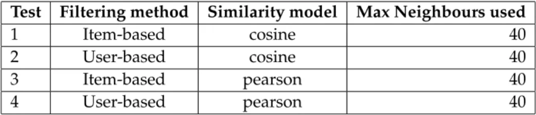
Built-in methods in Surprise were used to create the prediction algorithm. In table 2.1 the configurations for the different prediction algorithms are shown. All setups used a minimum of 1 neighbour for predictions.

Test Filtering method Similarity model Max Neighbours used

1 Item-based cosine 40 2 User-based cosine 40 3 Item-based pearson 40 4 User-based pearson 40

Table 2.1: Configurations for prediction algorithms

2.2.3 Evaluating the algorithms

Evaluation of the algorithms was done with the built-in function, evaluate(), in the Sur-prise library. Each test was run with all (10) test and training data combinations for each dataset. For both correlation evaluations (PCC and cosine similarity) and each dataset a mean value for the RMSE and MAE score was calculated based on the evaluation of the 10 different seeded partitions of the data. An average was used to prevent strong influ-ences from deviating scores in the case of bad data in the results.

(16)

Chapter 3

Results

The following structure will be used to present the results of the study:

Two sections are used showing results based on each of the similarity matrix struc-tures, Pearson correlation coefficient (Pearson) or cosine similarity (Cosine). For all datasets, user and item-based filtering will be compared side by side in a plot for each metric,

MAE or RMSE. The plot shows the average value of the 10 test runs. The lower the value, the better predictions have been made.

Following the plot of average scores there is another plot which shows the max devi-ation for the scores. This is the difference between the highest and lowest score of the 10 test runs for each dataset and filtering method. The lower the difference, the smaller the spread which has been observed between different test runs. This plot is included to give an idea of how much the tests varied which is relevant as we use an average value.

The full metrics of the tests are presented in appendix A.

3.1 Pearson

The following results were obtained using the Pearson method for the similarity matrix.

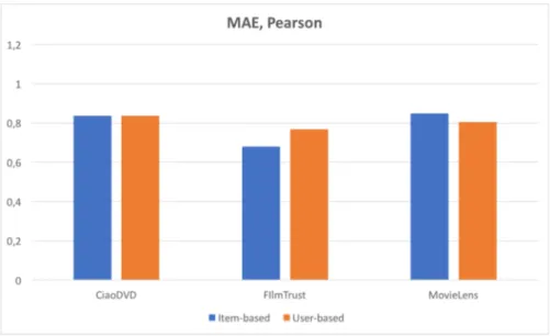
Figure 3.1: MAE, Pearson

(17)

The plot in figure 3.1 shows the results for the MAE scores. The plot shows a small advantage for item-based filtering for the FilmTrust dataset while there is an opposite ad-vantage for the MovieLens dataset. For the CiaoDVD dataset user and item-based based filtering score about the same.

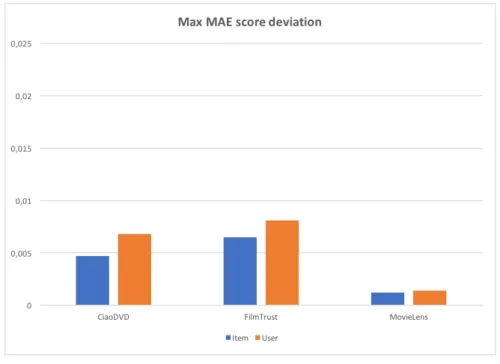
Figure 3.2: Max MAE score deviation for Pearson

The difference plot in figure 3.2 shows that the difference of the max and min value is less than 0.0215 for all the datasets. FilmTrust has highest value for user-based filtering. The scores have a deviation of around 3%. The plot also shows that there is a big differ-ence for user and item-based deviation for FilmTrust.

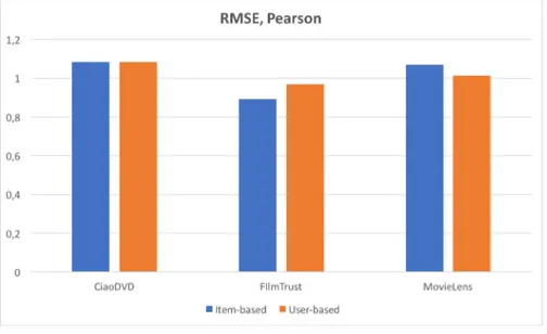
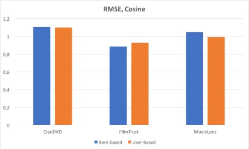
Figure 3.3: RMSE, Pearson

The RMSE scores, plotted in figure 3.3, give hints about the same trends as the MAE scores. The dataset for FilmTrust had better accuracy when item-based filtering was used

(18)

CHAPTER 3. RESULTS 11

and MovieLens had better accuracy when user-based was used. CiaoDVD had about the same accuracy for both filtering methods.

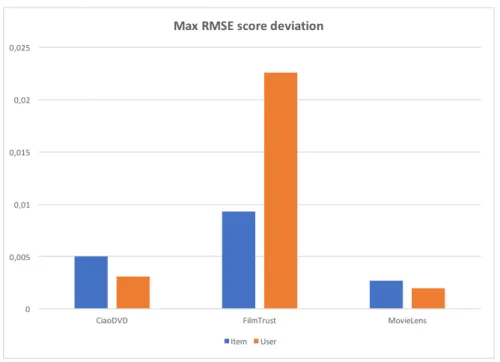
Figure 3.4: Max RMSE score deviation for Pearson

The difference plot in figure 3.4 shows the same max deviation for the FilmTrust dataset with less than 0.025 difference between the max and min values. The difference between the user and item-based approaches for the FilmTrust dataset which was observed in fig-ure 3.2 is present here as well.

(19)

3.2 Cosine

The following results were obtained using the cosine similarity method for the similarity matrix.

Figure 3.5: MAE, Cosine

In figure 3.5 the same trend which was observed for the pearson matrices in figure 3.1 are still visible. However, user and item-based filtering scored slightly closer to each other.

Figure 3.6: Max MAE score deviation for cosine

For the cosine similarity matrix, the difference between the max and min scores are much closer than for the Pearson similarity matrices. From figure 3.6 we see that the max score deviation is less than 0.01 points. However, there is a slightly lesser deviation for

(20)

CHAPTER 3. RESULTS 13

item-based filtering for all datasets. Notice that the big deviation for user-based filter-ing for the FilmTrust dataset which was observed when usfilter-ing the Pearson method is not present here.

Figure 3.7: RMSE, Cosine

The RMSE score using the cosine similarity matrix plotted in figure 3.7 shows the same trends as the RMSE score for the Pearson similarity matrix in figure 3.3.

Figure 3.8: Max RMSE score deviation for cosine

As opposed to the MAE score we see a slightly smaller deviation of the scores for user-based filtering. The deviation is less than 0.01 points which is very low.

(21)

Discussion

The discussion section has been divided into three parts with one part discussing our re-sults and how the study was conducted, one part talking about external dependencies and the last part analysing the current state of the art and the relevancy of the study. Figures 3.1 - 3.4 show a clear pattern where neither user nor item-based filtering has a clear advantage over the other, independent of error and correlation measurements (MAE, RMSE and Pearson, cosine). The results suggest that the choice of filtering method should be based on the data set. Exactly what properties of the data set that one should look for when determining filtering method is hard to say based on this study as it only contains 3 different ones with several differences (making it hard to pinpoint determining factors).

Our experiments show a clear correlation between the two error measurements where both give the same result for every dataset on what filtering method performed best. The MAE scores being lower than the respective RMSE ones across the board is expected as MAE can never produce a higher value than RMSE, only an equal one (if all errors have the same magnitude).

The maximum k value for the k-nearest neighbours algorithm which denotes how many items or users one makes the recommendations based on was chosen to be 40 in all tests. Choosing the optimal k value is not a simple task and there are many sugges-tions for how one should go about doing it but no agreed upon best method [18]. Us-ing cross validation with different k values and comparUs-ing results is one recommended method but this approach depends on the data set. Since different data sets are used in this study, different k values might be needed for the datasets to enable the system to perform at optimal capacity. Other ways of calculating an optimal k value are dis-cussed in [19]. Calculating an optimal k value for every data set was considered outside of this study’s scope and the default value of the Surprise library (40) was used instead. This value is, as stated, the maximum number of neighbours which the algorithm will consider. If there are not 40 users (or items) which are similar enough to be considered neighbours, Surprise will use a lower amount (to a minimum of 1). Using a different maximum k value may have an impact on the results if this study’s experiments are to be remade.

Every test result is a mean average of 10 runs where the training and test data sets were randomized. This method was used because it was a fair compromise when con-sidering its correctness and the scope of the study. One can naturally get a more sta-tistically sound value by averaging 1000 test runs instead of 10 but running the tests is

(22)

CHAPTER 4. DISCUSSION 15

time consuming (computationally) and it is hard to set a limit for how many data points are needed for a fair assessment. One more thing which our method doesn’t account for is outliers which can skew the mean considerably. However, only running each test 10 times allowed us to see that no big statistical outliers were present in the mean calcula-tions. This is shown in the figures (3.2, 3.4, 3.6, 3.8)

4.1 External dependencies

Two of the datasets, FilmTrust and CiaoDVD, were acquired from a scientific paper and not taken directly from their respective source. They were both collected by crawling the websites while these were online (they have been shut down at the time of writing). This makes it hard to control the correctness of the data. The dataset from CiaoDVD came in a non-compatible format for the python program so the data had to be processed and formatted which leaves room for human error.

An important attribute of the MovieLens dataset is that all users have made at least 20 ratings. There are no known similar minimum thresholds for the other datasets.

To raise the confidence of the drawn conclusions, more datasets should be used of varying sizes and from areas other than movie ratings. Initially the paper included a dataset from Yelp of restaurant reviews but because of its different data format and time restrictions, this dataset could not be used in this study.

We have no reason to doubt the Surprise software. All our tests have returned rea-sonable results and Surprise looks like a professionally built product for all intents and purposes. It is open source, actively maintained (latest commit was within 24 hours of writing (25-03-2017)), well documented and written by a Ph.D. student at IRIT (Toulouse Institute of Computer Science Research). To confirm the accuracy of the software, one can use the same data sets and algorithms of this study and input these into another work-ing recommender system and check if the results are identical.

4.2 State of the art and relevancy

Many companies use recommender systems today. Some bigger ones are Amazon, Face-book, Linkedin and Youtube. Finding out exactly what algorithms these companies use and how they are implemented has proven very difficult. There are two major reasons for this. One is that such information is part of their (often) closed source code. The other is that there is no simple answer to the question as most modern recommender systems are based on a plethora of algorithms. One famous case where this was displayed was the Netflix Prize, a contest for developing a better recommender system for Netflix with a price pool of a million dollars [20]. The best (winning) algorithms were in fact never implemented by Netflix as their huge complexity and engineering effort required over-shadowed the slightly better predictions they would bring [21].

The relevancy of the study can be questioned since its scope is quite narrow. Limiting itself to only comparing the accuracy of the two methods and dismissing other factors such as memory efficiency and computational demand/speed may make the results ir-relevant if one of the methods can’t ever be feasibly applied because of such limitations. However, even if such limitations do exist, this and similar studies could provide valu-able insight for if pursuing a solution to such limitations is worth putting effort into.

(23)

Conclusion

The study shows that neither the user nor the item-based filtering approach can be con-sidered better than the other when only comparing prediction accuracy (and ignoring other aspects such as memory usage and speed). When choosing between user or item based filtering, the choice should be based on the contents of the data set.

(24)

Bibliography

[1] Resnick P and Varian HR. Recommender systems. Communications of the ACM, 40: 56–58, 1997.

[2] Lampropoulos AS and Tsihrintzis GA. Machine Learning Paradigms. Intelligent Sys-tems Refernce Library. Springer International Publishing, 2015. ISBN 9783319191355. [3] MD Ekstrand, JT Riedl, and JA Konstan. Collaborative filtering recommender

sys-tems. Foundations and Trends in Human-Computer Interaction, 4:81–173, 2010.

[4] Resnick P, Iacovou N, Suchak M, Bergstrom P, and Reindl J. Grouplens: An open architecture for collaborative filtering of netnews. Proceedings of CSCW, 1994. [5] Zacharski R. A programmer’s guide to data mining, 2015.

[6] Linden G, Brent S, and York J. Amazon.com recommendations item-to-item collabo-rative filtering. Technical report, Amazon.com, 2003.

[7] Shani G and Gunawarda A. Evaluating recommender systems. Technical report, Microsoft Research, 2009.

[8] Wikipedia; Root mean-square deviation. https://en.wikipedia.org/wiki/root-mean-square_deviation, 2017. February 27, 2017.

[9] Wikipedia; Mean absolute error. https://en.wikipedia.org/wiki/mean_absolute_error, 2017. March 25, 2017.

[10] Guo G, Zhang J, and Yorke-Smith N. Trustsvd: Collaborative filtering with both the explicit and implicit influence of user trust and of item ratings. Proceedings of the Twenty-Ninth AAAI Conference on Artificial Intelligence, 2015.

[11] G. Guo, J. Zhang, and N. Yorke-Smith. A novel bayesian similarity measure for rec-ommender systems. In Proceedings of the 23rd International Joint Conference on Artificial Intelligence (IJCAI), pages 2619–2625, 2013.

[12] G. Guo, J. Zhang, D. Thalmann, and N. Yorke-Smith. Etaf: An extended trust an-tecedents framework for trust prediction. In Proceedings of the 2014 International Con-ference on Advances in Social Networks Analysis and Mining (ASONAM), pages 540–547, 2014.

[13] Harper F. M. and Konstan J. A. The movielens datasets: History and context. ACM Transactions on Interactive Intelligent Systems, 2016.

[14] Nicolas Hug. surpriselib.com, 2017. Mars 25, 2017. 17

(25)

[15] Open Source Initiative. opensource.org/licenses/bsd-3-clause, 2017. Mars 25, 2017. [16] Heckerman Chickering. Fast learning from sparse data. Microsoft Research, page 1,

1999.

[17] Evert AK. and Mattisson A. Rekommendationssystem med begränsad data. 2016.

[18] Researchgate.net. https://www.researchgate.net/post/how_can_we_find_the_optimum_k_in_k-nearest_neighbor, 2017. April 23, 2017.

[19] Byeoung U.Park Peter Hall and Richard J. Samworth. Choice of neighbor order in nearest-neighbor classification. The Annals of Statistics, Volume 36 Number 5, 2008. [20] Netflix Prize. http://www.netflixprize.com/, 2017. March 25, 2017.

[21] Mike Masnick. Why netflix never implemented the algorithm that won the netflix $1 million challenge. Technical report, Techdirt.com, 2009.

(26)

Appendix A

Metrics

A.1 CiaoDVD Metrics

CiaoDVD, Item-based, Cosine

Seed MAE RMSE Users in trainset Items in trainset 1 0.8495 1.1120 6287 6365 2 0.8450 1.1072 6359 6267 3 0.8461 1.1084 6417 6369 4 0.8475 1.1095 6362 6398 5 0.8461 1.1079 6321 6340 6 0.8480 1.1079 6344 6298 7 0.8462 1.1093 6329 6318 8 0.8487 1.1092 6341 6301 9 0.8448 1.1038 6368 6292 10 0.8467 1.1067 6372 6303 Mean 0.8469 1.1082 6350 6325.1

CiaoDVD, User-based, Cosine

Seed MAE RMSE Users in trainset Items in trainset 1 0.8454 1.1051 6287 6365 2 0.8408 1.1015 6359 6267 3 0.8441 1.1044 6417 6369 4 0.8415 1.1015 6362 6398 5 0.8386 1.0975 6321 6340 6 0.8429 1.1026 6344 6298 7 0.8444 1.1035 6329 6318 8 0.8428 1.1023 6341 6301 9 0.8436 1.1044 6368 6292 10 0.8419 1.1005 6372 6303 Mean 0.8426 1.1023 6350 6325.1 19

(27)

CiaoDVD, Item-based, Pearson

CiaoDVD, User-based, Pearson

A.2 FilmTrust Metrics

FilmTrust, Item-based, Cosine

Seed MAE RMSE Users in trainset Items in trainset 1 0.6757 0.8877 1267 875 2 0.6724 0.8813 1245 885 3 0.6780 0.8885 1253 905 4 0.6733 0.8823 1258 894 5 0.6721 0.8852 1266 893 6 0.6776 0.8911 1267 916 7 0.6747 0.8888 1274 913 8 0.6715 0.8811 1250 926 9 0.6768 0.8896 1266 895 10 0.6772 0.8864 1276 916 Mean 0.6749 0.8862 1262.2 901.8

(28)

APPENDIX A. METRICS 21

FilmTrust, User-based, Cosine

FilmTrust, Item-based, Pearson

FilmTrust, User-based, Pearson

(29)

A.3 MovieLens Metrics

MovieLens, Item-based, Cosine

MovieLens, User-based, Cosine

MovieLens, Item-based, Pearson

(30)

APPENDIX A. METRICS 23

MovieLens, User-based, Pearson

(31)

Code

B.1 main.py

from s u r p r i s e import KNNBasic from s u r p r i s e import Dataset , Reader from s u r p r i s e import e v a l u a t e , p r i n t _ p e r f import os

_ _ l o c a t i o n _ _ = os . path . r e a l p a t h ( os . path . j o i n ( os . getcwd ( ) , os . path . dirname ( _ _ f i l e _ _ ) ) ) t e s t d a t a _ p a t h = os . path . j o i n ( _ _ l o c a t i o n _ _ , ’ t e s t d a t a _ ’ )

t r a i n d a t a _ p a t h = os . path . j o i n ( _ _ l o c a t i o n _ _ , ’ t r a i n d a t a _ ’ )

r e a d e r = Reader ( l i n e _ f o r m a t = ’ u s e r item r a t i n g timestamp ’ , sep = ’ : : ’ ) # C r e a t e a f o l d s l i s t

t e s t _ f o l d s = [ ]

f o r num i n range ( 1 , 1 1 ) :

t u p l e = ( t r a i n d a t a _ p a t h + ’ { } ’ . format (num) , t e s t d a t a _ p a t h + ’ { } ’ . format (num ) ) t e s t _ f o l d s . append ( t u p l e )

p r i n t t e s t _ f o l d s

# Load t e s t and t r a i n data

p r i n t " # # # # Read t e s t and t r a i n data from f i l e s # # # # " data = D a t a s e t . l o a d _ f r o m _ f o l d s ( t e s t _ f o l d s , r e a d e r ) p r i n t " # # # # Read complete # # # # " sim_options = { ’ name ’ : ’ c o s i n e ’ , ’ user_based ’ : True } p r i n t " # # # # C r e a t i n g recommender system # # # # " a l g o = KNNBasic ( sim_options=sim_options , k =40) p r i n t " # # # # C r e a t i o n complete # # # # " f o r t r a i n s e t , t e s t s e t i n data . f o l d s ( ) :

p r i n t " # # # # NUMBER OF USERS IN TRAINSET : { } # # # # " . format ( t r a i n s e t . n _users ) p r i n t " # # # # NUMBER OF ITEMS IN TRAINSET : { } # # # # " . format ( t r a i n s e t . n_items )

# E v a l u a t e performances o f our a l g o r i t h m on t h e d a t a s e t . p e r f = e v a l u a t e ( algo , data , measures = [ ’RMSE’ , ’MAE’ ] ) p r i n t _ p e r f ( p e r f )

(32)

APPENDIX B. CODE 25

B.2 split_data.py

import os

import random

_ _ l o c a t i o n _ _ = os . path . r e a l p a t h ( os . path . j o i n ( os . getcwd ( ) , os . path . dirname ( _ _ f i l e _ _ ) ) ) # Path t o d a t a f i l e t o be s p l i t

f i l e _ p a t h = os . path . j o i n ( _ _ l o c a t i o n _ _ , ’ data/movielens/ml−1m/ r a t i n g s . dat ’ ) data = [ ] # Number o f l i n e s t o s k i p i n t h e beginning o f t h e f i l e s k i p _ l i n e s = 0 p r i n t " # # # # Reading data # # # # " with open ( f i l e _ p a t h , ’ r ’ ) as f : count = 0 f o r l i n e i n f : i f not ( count < s k i p _ l i n e s ) : data . append ( l i n e ) count = count + 1

p r i n t " # # # # Data read complete # # # # "

f o r num i n range ( 1 , 1 1 ) : random . seed (num)

p r i n t " # # # # S h u f f l e data # # # # " random . s h u f f l e ( data )

p r i n t " # # # # S h u f f l e data complete # # # # "

t e s t d a t a = open ( ’ t e s t d a t a _ { } ’ . format (num) , ’w’ ) t r a i n d a t a = open ( ’ t r a i n d a t a _ { } ’ . format (num) , ’w’ ) count = 0 p r i n t " # # # # Writing data # # # # " f o r l i n e i n data : i f ( count == 0 ) : t r a i n d a t a . w r i t e ( l i n e ) e l s e : t e s t d a t a . w r i t e ( l i n e ) count = ( count + 1 ) % 5 t e s t d a t a . c l o s e ( ) t r a i n d a t a . c l o s e ( ) p r i n t " # # # # Writing complete # # # # "

B.3 ciao_dvd_format.py

import os

_ _ l o c a t i o n _ _ = os . path . r e a l p a t h ( os . path . j o i n ( os . getcwd ( ) , os . path . dirname ( _ _ f i l e _ _ ) ) ) f i l e _ p a t h = os . path . j o i n ( _ _ l o c a t i o n _ _ , ’ data/CiaoDVD/movie−r a t i n g s . t x t ’ )

output = open ( ’ ciaoDVD_formated ’ , ’w’ ) output . w r i t e ( " userID , movieID , movieRating\n " ) with open ( f i l e _ p a t h , ’ r ’ ) as f :

(33)

f o r l i n e i n f :

s p l i t _ l i n e = l i n e . s p l i t ( ’ , ’ )

f o r m a t e d _ l i n e = " { } , { } , { } \ n " . format ( s p l i t _ l i n e [ 0 ] , s p l i t _ l i n e [ 1 ] , s p l i t _ l i n e [ 4 ] ) output . w r i t e ( f o r m a t e d _ l i n e )

(34)

Comparison of user and item-based collaborative filtering on sparse data

Comparison of user and

item-based collaborative filtering on

sparse data

ALEXANDER SÁNDOR

HARIS ADZEMOVIC

Comparison of user and item-based

collaborative filtering on sparse data

Abstract

Sammanfattning

Contents

Chapter 1

Introduction

1.1

Background

1.2

Datasets

1.3

Surprise

1.4

Purpose

1.5

Research question

1.6

Scope and constraints

Chapter 2

Method

2.1

Data handling

2.2

Conducting the tests

Chapter 3

Results

3.1

Pearson

3.2

Cosine

Discussion

4.1

External dependencies

4.2

State of the art and relevancy

Conclusion

Bibliography

Appendix A

Metrics

A.1

CiaoDVD Metrics

A.2

FilmTrust Metrics

A.3

MovieLens Metrics

Code

B.1

main.py

B.2

split_data.py

B.3

ciao_dvd_format.py