Forecasting Non-Maturing Liabilities

(1)

IN

DEGREE PROJECT MATHEMATICS, SECOND CYCLE, 30 CREDITS

,

STOCKHOLM SWEDEN 2017

Forecasting Non-Maturing

Liabilities

ADRIAN AHMADI-DJAM

SEAN BELFRAGE NORDSTRÖM

KTH ROYAL INSTITUTE OF TECHNOLOGY SCHOOL OF ENGINEERING SCIENCES

(2)

(3)

Forecasting Non-Maturing

Liabilities

ADRIAN AHMADI-DJAM

SEAN BELFRAGE NORDSTRÖM

Degree Projects in Mathematical Statistics (30 ECTS credits)

Degree Programme in Applied and Computational Mathematics (120 credits) KTH Royal Institute of Technology year 2017

Supervisor at Carnegie: Kristoffer Straume Supervisor at KTH: Pierre Nyquist

(4)

TRITA-MAT-E 2017:11 ISRN-KTH/MAT/E--17/11--SE

Royal Institute of Technology

School of Engineering Sciences

KTH SCI

SE-100 44 Stockholm, Sweden URL: www.kth.se/sci

(5)

2

Abstract

With ever increasing regulatory pressure financial institutions are required to carefully monitor their liquidity risk. This Master thesis focuses on asserting the appropriateness of time series models for forecasting deposit volumes by using data from one undisclosed financial institution. Holt-Winters, Stochastic Factor, ARIMA and ARIMAX models are considered with the latter being the one with best out-of-sample performance. The ARIMAX model is appropriate for forecasting deposit volumes on a 3 to 6 month horizon with seasonality accounted for through monthly dummy variables. Explanatory variables such as market volatility and interest rates do improve model accuracy but vastly increases complexity due to the simulations needed for forecasting.

(6)

3

Sammanfattning

Med ständigt ökande krav på finansiella institutioner måste de noga övervaka sin likviditetsrisk. Detta examensarbete fokuserar på att analysera lämpligheten av tidsseriemodeller för

prognoser inlåningsvolymer med hjälp av data från en ej namngiven finansiell institution.

Holt-Winters, Stochastic Factor, ARIMA och ARIMAX modellerna används, där den senare uppvisar bäst resultat. ARIMAX modellen är lämplig för prognoser av inlåningsvolymer på en 3-6 månaders tidshorisont där hänsyn till säsongseffekter tagits

genom månatliga dummyvariabler. Förklaringsvariabler såsom marknadsvolatilitet

och räntor förbättrar modellens prognosticeringsprecision men ökar samtidigt

(7)

4

Acknowledgements

We would like to extend our sincerest thanks to our classmates, friends, family and KTH faculty. Without you the completion of this thesis would not be possible. An extra big thank you to our supervisor Pierre Nyquist who provided guidance throughout our work.

Adrian Ahmadi Sean Belfrage

(8)

5

List of Figures

Figure 1: Jan13-Nov16. Deposits for segment A3 normalised to 100 at the start of the period. ... 25

Figure 2: Jan13-Nov16. One time differentiated logarithm of deposits for segment A3. 5 day interval between observations. ... 25

Figure 3: Jan13-Nov16. Distribution of differentiated logarithm of deposits for segment A3. 5 day interval between observations. ... 26

Figure 4: Jan13-Nov16. Distribution of differentiated logarithm of deposits for segment A3. Overlapping 5 day interval between observations. ... 27

Figure 5: Jan13-Nov16. Quantile-quantile plot of logarithm of deposits for segment A3. Overlapping 5 day interval between observations. ... 28

Figure 6: Jan13-Nov16. Box plot of differentiated logarithm of deposits by day of the week for segment A3. 5 day interval between observations. Marker indicates median values. ... 28

Figure 7: Jan13-Nov16. Box plot of differentiated logarithm of deposits by quarter for segment A3. 5 day interval between observations. Marker indicates median values. ... 29

Figure 8: Jan13-Nov16. Box plot of differentiated logarithm of deposits by month for segment A3. 5 day interval between observations. Marker indicates median values. ... 29

Figure 9: Jan13-Nov16. Differentiated logarithm of deposits for segment A1. 21 day overlapping interval between observations. ... 30

Figure 10: Jan13-Nov16. ACF plot for differentiated logarithm of deposits for segment A1. 21 day overlapping interval between observations. ... 30

Figure 11: An example of the simulated short term market rate paths from the Vasicek model. Each time step is of length 5 working days. ... 32

Figure 12: An example of the simulated volatility from the GARCH(1,1) model. Each time step is of length 5 working days. ... 33

Figure 13: Quantile-quantile plot for the residuals of the residuals of the GARCH(1,1) model. ... 34

Figure 14: ARIMAX(1,1,1) model forecast for segment A with 1 day time interval. MAPE of 9.9%. ... 36

Figure 18: SARIMAX(0,0,0)x(0,1,5)21 model forecast for segment A with 1 day time interval. MAPE of 7.8%. ... 37

(10)

7

Figure 19: SARIMAX(0,0,0)x(0,1,5)21 model residual ACF for segment A with 1day time

interval. ... 37

Figure 20: Holt Winters model forecast for segment A with 5 day time interval. MAPE of 9.6%. ... 38 Figure 21: SF model forecast for segment A with 5 day time interval. MAPE of 15.6%. ... 39 Figure 22: SF model forecast for segment A with 10 day time interval. MAPE of 9.9%. ... 39 Figure 23: ARIMA(6,1,7) model forecast for segment A with 5 day time interval. MAPE of 7.9%. ... 40

Figure 24: SARIMA(1,1,1)x (1,0,1)23 model forecast for segment A with 10 day time interval.

MAPE of 14.5%. ... 41

Figure 25: ARIMAX(6,1,7) model forecast for segment A with 5 day time interval. MAPE of

4.5%. ... 42

Figure 26: SARIMAX(0,0,0)x(0,1,1)4 model forecast for segment A with 5 day time interval.

MAPE of 7.2%. ... 44

Figure 27: ARIMAX(6,1,7) model one period ahead forecast for segment A with 5 day time

interval. MAPE of 6.8% with monthly dummies. ... 46

Figure 28: SARIMAX(0,0,0)x(1,1,1)21 model one period ahead forecast for segment A with 1

day time interval. MAPE of 14.5%. ... 46

Figure 29: ARIMAX(6,1,7) model one period ahead forecast for segment A with 5 day time

interval. MAPE of 5.7% without monthly dummies. ... 46

Figure 30: SARIMAX(0,0,0)x(1,1,1)21 model one period ahead forecast for segment A with 1

(11)

8

1. Introduction

1.1 Background

During the 2008 financial crisis Lehman Brothers did not go bankrupt because their shareholder’s equity turned negative. Instead, what really happened was that they did not have sufficient liquidity to meet their near-term commitments as pointed out by for example Ball (The Fed and Lehman Brothers, 2016). The crisis showed the importance of stable funding and sufficient liquidity in the financial sector. The liquidity freeze quickly spread to the rest of the economy placing many companies in default. Regulators have since responded by placing liquidity and stable funding in the financial sector at the very top of their agenda. This has made deposit funding with long behavioral maturity more attractive from a regulatory perspective.

Deposit funding is associated with a specific type of risk, i.e. the risk that arises from the optionality of withdrawing deposits at any point without prior notice. To mitigate this risk the financial institutions’ treasury departments have to closely monitor the liquidity position to ensure that all commitments can be met and that there is sufficient liquidity for managing the day-to-day business.

1.2 Problem Discussion

For financial institutions deposit funding is a valuable tool, however the modelling and forecast of future deposit volumes can be a complex task. The means for liquidity management varies greatly from institution to institution even though the financial supervisory authorities have issued detailed guidelines and regulations. One metric of regulatory interest is the Liquidity Coverage Ratio, LCR, which describes what level and type of liquidity a financial institution is required to hold against the deposits of a certain type of client. One way to approach the problem of modeling deposits is to divide it into a stable (“sticky”) part and a volatile part. The idea is that the sticky part can be assumed to be fairly constant or growing slowly over time while the volatile part needs to be modeled separately.

The stableness of deposits is something that has been frequently investigated, for example Leonart Matz (How to Quantify and Manage Liability Stickiness, 2009) analysed a number of qualifications he hypothesized should define “stickiness” of non-maturing liabilities. The qualifications include for example whether the depositor is sophisticated, or if the deposit is insured. Matz concluded that modelling of deposit volumes is a complex task and that there is no complete formula for quantifying stickiness of deposits.

Earlier studies have used a range of different methods to model deposits or cash flows at financial institutions. Jaroslaw Bielak et al. (Modelling and Forecasting Cash Withdrawals in the Bank, 2015) investigated optimal forecasting methods for cash withdrawal in a Polish bank. The authors utilised both statistical and machine learning (artificial neural networks) methods in order to find good deposit forecasts. The conclusion reached was that an ARIMAX model with integer valued factors variables for day of the week (1, 2,…, 5) , day of the month (1, 2,…,

(12)

9 31) and month of the year (1, 2,…, 12) as explanatory variables yielded the best out-of-sample performance as determined by the mean average percentage error.

Helena von Feilitzen (Modeling Non-maturing Liabilities, 2011) modelled deposit volumes at a large Swedish bank by using the bond replication method in which the liabilities are modelled as portfolios of bonds with a combination of maturity dates. The author concluded that it was indeed possible to model deposits through the bond replication method, but that a more advanced option adjusted spread model would be preferable.

To the best of our knowledge there are no studies analyzing the specific use of time series methods in order to model deposit volumes. Furthermore time series analysis on segmented deposit data through client level detail allows for a diversified study in terms of methodology.

1.3 Problem Formulation

The hypothesis investigated in this study is that time series analysis would be an appropriate means of forecasting deposit volumes at financial institutions. Such analysis would allow for better understanding of the expected volatility and required size of operational liquidity at any given point in time. Thus the broad research question can be formulated as:

- To what extent are time series models appropriate for forecasting deposit volumes? Here, appropriate is subject to a certain degree of subjectivity includes, but is not limited to; business sense of the model output, size of forecasting error, out-of-sample performance and user friendliness.

To answer the research question a range of different time series models are analysed and compared with the objective of finding appropriate time series models. The specific models investigated are Holt Winters model, Stochastic Factor model, ARIMA models and ARIMAX model where explanatory variables are included. Explanatory variables assumed to affect deposit volumes are in this study: Stock index volatility, market interest rate and deposit interest rate. These variables are investigated together with time series analysis in order to facilitate models of deposit volumes.

The statistical software utilised to answer the question is R. For pre-processing and graphical purposes Microsoft Power BI and Microsoft Excel are used.

1.4 Study Aim and Limitations

The purpose of this study is to analyse the appropriateness of using time series to forecast the deposit volumes for a specific undisclosed financial institution. The application in practice of

successfully forecasting deposit volumes is to allow for a more efficientallocation of funds. An

additional purpose with this study is to analyse the appropriateness of segmenting deposits by client characteristics with the hypothesis that similar clients will behave in the same way.

(13)

10 One limitation of the study is that only a subset of forecast lengths can be investigated. The primary focus is put on 3-6 months forecasts to allow for a sufficiently long period in the perspective of liquidity planning. This furthermore corresponds to a statistically reasonable ~10% of out of sample data when observing the entire set of data. To further investigate the predictive power of the time series models shorter time intervals will also be analysed.

Further limitations of the study are that only a subset of time series models will be considered, the data used will only be from one financial institution and for a specific period of time. Thus, one should be careful about applying the conclusions drawn in this thesis to other types of institutions.

1.5 Thesis Structure

This thesis is organised as follows. Section 2 starts with a thorough review of previous research on deposit modelling. In Section 3 the theory for the main models used is presented. In Section 4 the data and the pre-processing required to transform the data into a desired format are presented, as well as the specific models used for forecasting. The section concludes with descriptive statistics and example of simulations of exogenous variables. Results for the different models are presented and commented on in Section 5. In Section 6 the results are discussed and the thesis is concluded.

(14)

11

2. Previous Research

In this section previous studies on similar problems in the area of deposit volumes and time series forecasting is presented. The previous research is reviewed to put the current work in the area into context and is used as inspiration for the methodology in this thesis.

A report from the federal deposit insurance corporation (Study on core deposits and brokered deposits, 2011) analyse core deposits, otherwise known as stable deposits or sticky deposits. These types of deposits are not defined by statute, however there are definitions created for analytical purposes in order to better understand stable funding sources in depository institutes. Stable deposits are rarely determined by a single characteristic, such as whether a deposit is insured, but rather by a multitude of affecting factors. The federal deposit insurance corporation defines stable deposits by the deposits from certain stable client accounts with amounts below the deposit insurance level ($250,000 in the U.S.) (Federal deposit insurance corporation, 2011, pp. 4-5). However the article further describes that stable deposit accounts sometimes display volatile patterns and that accounts classified as volatile (for example with deposits above the insurance level) sometimes are more stable.

Leonard Matz (How to Quantify and Manage Liability Stickiness, 2009) analyses what characterizes a deposit or liability as stable. Matz argues that core liabilities are liabilities that are less likely to disappear during a stressed liquidity scenario and describes eight characteristic that increases liability stickiness; 1) The deposit is insured; 2) The liability is backed by quality collateral; 3) The deposit funds are controlled by the owner rather than by an agent; 4) The depositor has other commitments with the bank; 5) The depositor is a net borrower; 6) The depositor lacks internet access to the funds; 7) The depositor is “unsophisticated”, e.g. a private person rather than a financial institution; 8) The deposits are obtained directly rather than from a third party. Furthermore Matz argues that the maturity of time or term liabilities is an important factor for stickiness that should be kept separate from the above eight factors as it is conceptually different. Matz concludes that there is no easy formula that quantifies stickiness, rather it is a continuous scale that depends on liquidity stress scenario and degree.

Jaroslaw Bielak et al. (Modelling and Forecasting Cash Withdrawals in the Bank, 2015) investigate optimal forecasting methods for daily cash withdrawal in a Polish bank utilising both statistical time series models and machine learning methods in the form of artificial neural networks. The authors argue that both insufficiency and excess of liquidity can be costly and that proper liquidity forecasting methods are required for this purpose. Bielak et al. analyse the bank customers’ daily cash withdrawal for the period July 2012 to April 2014, summing up to a data set of 461 data points which exclude weekends and bank holidays. For modelling purposes the natural logarithm of cash withdrawals is used. The data set is further split into five subsets, one larger training set with 378 data points and four test (or forecasting) sets with 20 or 21 data points each. The models utilised are created from the training set and forecast tested with the test sets as comparison. To determine the optimal model the forecast accuracy of each model is measured and Bielak et. al define the forecast accuracy as the mean absolute percentage error in the out of sample period. The authors first test the best ARIMA model, as

(15)

12 determined by the AIC criterion, and conclude that the forecast accuracy was poor for all testing periods. For the second model the authors first utilise Kruskal-Wallis test to determine statistically significant differences in withdrawals for individual days of the week (DW), days in the month (DM) and months in the year (MY). Ordinary least square approach is used to find the polynomials for DW, DM and MY respectively which best fit cash withdrawals. The polynomials are used as independent variables in an ARMAX time series model (ARMA model with exogenous inputs) which is used to forecast cash withdrawals. Furthermore the withdrawals for the tenth day of the month were found to exhibit outlier behaviour and a dummy variable for this day is included. The ARMAX model approach resulted in mean absolute percentage errors for the four test periods of approximately 20%, significantly lower than observed for the machine learning approach, particularly for later test periods. The authors conclude that forecasting cash withdrawals is a complex task, and that the independent calendar variables (DM, DW and MY) affected the cash withdrawals in a none-linear fashion.

Kaj Nyström (On deposit volumes and the valuation of non-maturing liabilities, 2008) provides a mathematical framework for modelling non-maturing liabilities. The article focus on three model methodologies; firstly market rates, secondly deposit rates and thirdly deposit volumes, of which the latter category is of particular interest in this study. Nyström models deposits in a bank by assuming deposits can be put in a transaction account or a finite amount of different savings accounts. Furthermore, there is an option to change the deposits between the different accounts. Nyström proposes a behaviour model where the option to transfer a deposit to another account is used whenever stochastic processes, depending on market and deposit rates as well as the deposited amounts, exceeds “the client specific strike price”. The model is simplified by excluding the possibility of transferring deposits outside the bank or transfers into the bank. This specific way of modelling deposit volumes is according to Nyström not a common method, instead the author states that an autoregressive model with exogenous independent variables is most commonly used to model deposit volumes.

The use of time series methods to forecast financial data is commonly found in the literature. Wen-Hua Cui et al. (Time Series Prediction Method of Bank Cash Flow and Simulation Comparison, 2014) test the predictive values of the moving average and exponential smoothing methods on bank cash flows. The authors reach the conclusion that for real time cash flows in a commercial bank the best method tested is the exponential smoothing method of order two.

Castagna & Manenti (Sight Deposits and Non-Maturing Liabilities Modelling, 2013) set out to review different approaches for the modelling of non-maturing deposits suggested in literature and from business practices. First a comparison between the bond replication method and the Stochastic Factor, SF, approach is made. The main ideas behind the different methods, identifying how deposit volumes are linked to risk factors such as interest rates, are similar. However, it is concluded that the SF approach is superior because of four reasons. Firstly, the SF approach accounts for the stochastic evolution of the risk factors. Secondly, it allows joint evaluation of deposit value and the future cash flows – providing a consistent framework. Thirdly, it is possible to include behavioural functions and consequently linking deposit volumes to the stochastic evolution of the risk factors. Finally, under the SF approach it is

(16)

13 possible to account for bank-runs. In the article the authors only consider the interest rates and deposit rates to be risk factors. The SF approach requires one stochastic model for each of the risk factors and one for the evolution of deposit volumes. A CIR++ model (Castagna & Manenti, 2013, p. 3) with parameter estimation through the use of Kalman filter, is used for the market interest rates and the deposit rate is modelled as a linear function of the market interest rate. Furthermore, a range of different models for deposit volumes are considered, with examples presented using monthly Italian deposits data from the years 1999-2012. First a linear behavioural function is considered, where the logarithm of the deposits is assumed to be a linear function of the logarithm of the lagged deposits and changes in the risk factors. The authors argue that a time trend component, of suitable form, could be included, but claim to be interested in how deposit volume evolution is linked only to rates’ changes. The linear behavioural

function renders functions that are well-fitted to the in-sample data, with an R2 of 0.99.

Moreover the authors suggest a non-linear behaviour model under the assumptions that each depositor changes balance as a fraction of income, that there is a depositor specific interest rate strike level E such that when the market interest rate is above E the depositor will allocate a higher proportion of their income to other investments and that there is a depositor specific rate strike level F such that when the deposit rate is above F the depositor will allocate a higher proportion of their income towards deposits. The authors consider a Gamma distribution for the

cumulative density of the average customer’s strike levels and the corresponding in-sample R2

is 0.97. In the final model bank run effects are accounted for by the inclusion of a component for the credit spread for the depository institutions. Finally the authors use Monte Carlo simulations of the risk factors to model the future deposit volume paths, and consequently presenting upper and lower bound for the deposit volumes.

In Modeling Non‐maturing Liabilities (von Feilitzen, 2011) the author sets out to model deposits at a large Swedish bank in order to improve liquidity and interest rate risk management. The author seeks a model for which the modelling error is as small as possible, the interest rate risk is as low as possible, the profit is as high as possible and the model should be readily implemented by the bank. The main focus of the thesis is on replicating portfolio approaches, although the Option Adjusted Spread (SF) model is discussed as a feasible alternative. The replicating portfolio is essentially a suitably chosen portfolio of fixed income assets that matches the expected cash flows equivalent to changes in deposit volume. One of the replicating portfolios is obtained by minimising the standard deviation of the margin between the portfolio return and the deposit rate, the other one by maximising the Sharpe ratio. An alternative version of deposit rate is formulated as a moving average of market rates and is also considered. The weights of the optimised portfolio are also subject to some naïve liquidity constraints to account for large withdrawals. The author concludes that a portfolio replication approach is indeed feasible, but also suggests a more advanced SF approach for future research as this model easier account for stickiness and allows for a deposit interest rate model.

In Italian deposits time series forecasting via functional data analysis (Piscopo, 2010) the author aims to develop a Functional Data Model for forecasting Italian deposit time series. The author uses a singular value decomposition to fit a time series model based only on historical values of deposits with specific focus on seasonality analysis. More specifically, the paper focuses on

(17)

14 analysing the seasonality in, and difference between, years. Monthly time series data for Italian deposits for the years 1998 to 2008 are used and Piscopo finds evidence for difference in seasonality between years. Furthermore, the functional model is found to give slightly smaller residuals than traditional time series models. For sake of forecasting the classical ARIMA process is used. To conclude the authors recommend the functional data analysis to be a complementing tool to the more traditional analysis carried out in this paper.

The previous research presented in this section provides a baseline for the methodology in this thesis. The article by Jaroslaw Bielak et al. (Modelling and Forecasting Cash Withdrawals in the Bank, 2015) is of particular interest and much of the methodology is reproduced in this study, however for deposit volumes rather than deposit withdrawals.

(18)

15

3. Theoretical background

In this section the theories behind the models and tests used to analyse the data are presented and discussed. The section is organised in the order of the time series models utilised in this study: 1) Holt-Winters model; 2) Multiple Linear Regression models; 3) ARIMA models; 4) Modified ARIMA models. Furthermore the theory behind GARCH time series models required for explanatory variable simulation is presented in 5) GARCH and a test for stationarity in 6) Augmented Dickey Fuller test.

3.1 Holt-Winters’ Exponential Smoothing with Seasonality

A simple time series for forecasting purposes is Holt-Winter’s exponential smoothing with seasonality as seen in for example Hyndman et. al. (Forecasting: principles and practice, 2013). For simplicity this will be referred to as the Holt-Winters’ model throughout this thesis. The main idea behind the model is that an exponential moving average gives a good approximation of future values. In addition to this the algorithm also allows for a trend and seasonality. Mathematically this can be formulated as:

𝐼𝑛𝑖𝑡𝑖𝑎𝑙 𝑉𝑎𝑙𝑢𝑒𝑠 { 𝐿_𝑠 =1 𝑠∑ 𝑦𝑖 𝑠 𝑖=1 𝑏_𝑠 =1 𝑠[ 𝑦_𝑠+1− 𝑦₁ 𝑠 + 𝑦_𝑠+2− 𝑦₂ 𝑠 + ⋯ + 𝑦_2𝑠− 𝑦_𝑠 𝑠 ] 𝑆_𝑖 = 𝑦_𝑖 − 𝐿_𝑠, 𝑖 = 1, … , 𝑠 (1)

where 𝑦𝑡 is the variable of interest at time t. For 𝑡 > 𝑠 we caclulate:

𝐿𝑒𝑣𝑒𝑙: 𝐿_𝑡 = 𝛼(𝑦_𝑡− 𝑆_𝑡−𝑠) + (1 − 𝛼)(𝐿_𝑡−1+ 𝑏_𝑡−1)

𝑇𝑟𝑒𝑛𝑑: 𝑏𝑡 = 𝛽(𝐿𝑡− 𝐿𝑡−1) + (1 − 𝛽)𝑏𝑡−1

𝑆𝑒𝑎𝑠𝑜𝑛: 𝑆𝑡 = 𝛾(𝑦𝑡− 𝐿𝑡) + (1 − 𝛾)𝑆𝑡−𝑠

𝐹𝑜𝑟𝑒𝑐𝑎𝑠𝑡: 𝑦̂𝑡+1= 𝐿𝑡+ 𝑏𝑡+ 𝑆𝑡+1−𝑠

(2)

for all available observations. Above 𝛼, 𝛽 and 𝛾 are coefficients to be chosen. This can be done by minimising sum of squared errors.

All subsequent forecasts are calculated as:

𝑦̂_𝑛+𝑘 = 𝐿_𝑛 + 𝑘 ∙ 𝑏_𝑛 + 𝑆𝑛+𝑘−𝑠 (3)

3.2 Multiple Linear Regression

In regression analysis one seeks to establish a linear relationship between a dependent variable and one or more independent variables, or covariates. This can be mathematically formulated as:

(19)

16

where n is the number of observations, 𝑦𝑖 is the i:th observation of the dependent variable, 𝑥𝑖 =

(𝑥𝑖0 … 𝑥𝑖𝑘) is a row vector containing the i:th observation for the 𝑘 + 1 covariates, 𝑒𝑖 the

residual of the i:th observation and 𝛽 = (𝛽₀ … 𝛽_𝑘)𝑇_{is a column vector containing the 𝑘 + 1}

regression coefficients. The aim is to estimate the coefficients such that the square of the residuals is minimised. This is done by employing the Ordinary Least Squares, OLS, method.

In order for OLS to render meaningful results one needs to make a series of assumptions (Lang, 2014). The main assumptions are listed below.

 Linear dependence between independent variable and covariates  No multicollinearity

 Homoscedasticity

 Independent and identically distributed residuals with mean zero

The first assumption is not very restrictive as one can easily transform the dependent variable or the covariates to a different form if one suspects that the relationship of the “original” variables is non-linear. To validate the model the residuals will be checked for homoscedasticity and normality by plotting the residuals and a quantile-quantile graph respectively.

3.3 ARIMA

The autoregressive moving average (ARMA) model is a statistical model utilised for fitting and forecasting stationary time series. The ARMA fit a model to data based on the previous development of the time series. The autoregressive (AR) part of the model specifies the time series’ variable’s dependency on its own lagged values, whereas the MA part specifies the regression error’s dependency on previous regression errors.

For non-stationary time series an autoregressive integrative moving average (ARIMA) model can be used. The “integrated” part of the ARIMA model is a differencing process to reduce a time series to stationarity, thus reducing the required model to an ARMA model. If a time series follows an ARIMA(p,d,q) process the variable can be predicted and fitted using an ARIMA model of the same order, where p denotes the order of autoregressive part, d the order of the integrated part and q the order of the moving average part. An ARIMA(p,d,q) process can easily be reduced to an ARMA(p,q) process by differentiating the time series d times. The general form of an ARIMA model can be stated as:

(1 − ∑ 𝜙_𝑖𝐵𝑖 𝑝 𝑖=1 ) (1 − 𝐵)𝑑_𝑦 𝑡 = (1 + ∑ 𝜃𝑗𝐵𝑗 𝑞 𝑗=1 ) 𝜖_𝑡 (5)

where 𝑦_𝑡 is the time series data and 𝜖_𝑡 ∈ 𝑊𝑁(0, 𝜎2). The 𝜙_𝑖’s are the coefficients in the AR

polynomial of order 𝑝, 𝜃𝑗 are the coefficients in the MA polynomial of order 𝑞 and (1 − 𝐵)𝑑 is

(20)

17

(1 + 𝜃₁𝑧 + ⋯ + 𝜃_𝑞𝑧𝑞_{) have no common roots. 𝐵 is the backward shift operator which is}

characterised by:

𝐵𝑘_𝑦

𝑡= 𝑦𝑡−𝑘 (6)

There are various ways to determine the order of the most suitable ARIMA model for a given time series. The visualization of the autocorrelation and partial autocorrelation functions are which can give indications on the required order. The method utilized in this study is to iterate over different choices of 𝑝 and 𝑞, and then choosing the model which yields the lowest Aikake’s Information Criterion, AIC, values;

𝐴𝐼𝐶 = −2 ln(𝐿) + 2𝑚 (7)

where 𝐿 is the maximum value of the likelihood function for the model and 𝑚 is the number of estimated parameters. The likelihood function is based on the model residuals. The parameter value of d can be chosen by observing when stationarity arise by plots, and through an Augmented Dickey Fuller test, by increasing d equal to 0, 1, 2 etc.

The estimation of the model parameters, 𝜃_𝑖 and 𝜙_𝑗, can be done in several ways. A common

method is to use the maximum likelihood estimation which maximizes the probability of making the observations given the fitted parameters. Maximum likelihood estimation is the method used in the statistical software R, whilst minimizing the root of the squared regression error as the starting point for iteration.

As in the case of a linear regression the residuals from a fitted ARIMA model must satisfy certain criteria such, as lack of autocorrelation, and i.i.d. distribution.

3.4 Modified ARIMA Models

The seasonal ARIMA (SARIMA) model is a modification of the ARIMA model where a

seasonal component of the time series is introduced. A SARIMA(𝑝, 𝑑, 𝑞)(𝑃, 𝐷, 𝑄)𝑠 model can,

analogous with the ARIMA(𝑝, 𝑑, 𝑞) model, be written as:

(1 − ∑𝑝 𝜙_𝑖𝐵𝑖 𝑖=1 )(1 − ∑𝑃𝑖=1Φ𝑖𝐵𝑖𝑠)(1 − 𝐵)𝑑(1 − 𝐵𝑠)𝐷𝑦𝑡= = (1 + ∑ 𝜃𝑗𝐵𝑗 𝑞 𝑗=1 ) (1 + ∑ Θ𝑗𝐵𝑗𝑠 𝑄 𝑗=1 ) 𝜖𝑡 (8)

where Θ_i is the seasonal autoregressive polynomial coefficients, Φ_i is the seasonal moving

average polynomial coefficients and (1 − 𝐵𝑠₎𝐷_{is the seasonal differencing of order 𝐷. The}

order of d and D is chosen in the same fashion as for ARIMA models through observing the

stastionarity of (1 − 𝐵)𝑑_{(1 − 𝐵}𝑠₎𝐷_𝑦

(21)

18

either be assumed to be a logical period of time (e.g. 1 year, 𝑠 = 12 for monthly data) or be

derived from observing ACF or PACF plots.

A further modification of the ARIMA model is the ARIMAX model which allows for incorporation of exogenous variables as explanatory variables (Williams, 2001). The ARIMAX model with one exogenous variable can be written:

(1 − ∑ 𝜙_𝑖𝐵𝑖 𝑝 𝑖=1 ) (1 − 𝐵𝑑_)𝑦 𝑡= (1 + ∑ 𝜃𝑗𝐵𝑗 𝑞 𝑗=1 ) 𝜖_𝑡+ ∑ 𝜂_𝑘𝑑_𝑡,𝑘 𝑏 𝑘=1 (9)

where 𝜂𝑘 are the parameters for the b exogenous variables 𝑑𝑡,𝑘 where k = 1, 2, ... b. The

coefficients are estimated by maximizing the likelihood function analogously as for ARIMA models.

3.5 GARCH

In order to model the volatility of the stock market a GARCH(1,1) model is used (Bollerslev, 1986). It is understood that the GARCH(1,1) model is not always the model with the best performance but it will suffice for the purpose of this thesis. The model can be mathematically formulated as:

𝜎_𝑡+12 _{= 𝜔 + 𝛼𝑅}

𝑡2+ 𝛽𝜎𝑡2, 𝜔 > 0, 𝛼 ≥ 0, 𝛽 ≥ 0, 𝛼 + 𝛽 < 1 (10)

where 𝜎_𝑡 is the volatility at time t, 𝑅_𝑡 is the logarithmic return at time t and 𝛼, 𝛽 and 𝜔 are

constant coefficients. The coefficients are typically estimated by employing the maximum likelihood approach.

3.6 Augmented Dickey Fuller Test

Augmented Dickey Fuller test is utilised to determine stationarity of a time series (Fuller, 1976). The test is carried out with the null hypothesis of non-stationarity (a unit root present) in a time series sample. The test is applied to a model on the form:

Δ𝑦_𝑡 = 𝛼 + 𝛽𝑡 + 𝛾𝑦_𝑡−1+ 𝛿₁Δ𝑦_𝑡−1+ ⋯ + 𝛿_𝑝−1Δ𝑦_{𝑡−𝑝+1}+ 𝜖_𝑡 (11)

where 𝛼, 𝛽, 𝛾, 𝛿 are coefficients. Under the null hypothesis 𝛾 = 0 and the alternative hypothesis is that 𝛾 < 0. The test statistic 𝛾̂/𝑆𝐸(𝛾̂) is compared to the relevant critical value for the Dickey Fuller test.

(22)

19

4. Method

In this section the methodology carried out in completing this thesis is presented. The section is initialised by presenting 1) the data sources available for the thesis; 2) the data treatment and pre-processing required in transforming the data for further tests; 3) description of variables of interest for this study; 4) the modelling approach for the specific time series models utilised in this thesis.

Furthermore, theory required for explanatory variable simulation is presented: 5) Volatility Simulation; 6) Market Rate Simulation.

Additionally model specific theory required in this thesis is presented in 7) Model Aggregation; 8) Model Validation.

The section is concluded by presenting 9) Descriptive Statistics and 10) Explanatory Variable Simulation.

Throughout the following sections working days is referred to as and unless otherwise stated the data is from non-overlapping time periods.

4.1 Data Sources

The data used in this study is four years of daily observations of deposit volume for each client. Further client specific data, such as type of client, total assets under management and average deposit rate is included on a daily basis.

The close price of the OMXS30 index, which is used to calculate the volatilities of the OMXS30 index, is obtained from Nasdaq.

One month STIBOR has been chosen as the proxy for market rate in this study and is obtained

from the Swedish Riksbank.1

4.2 Data Treatment and Pre-processing

In order to get the data on a convenient form a very extensive pre-processing work has to be carried out. As specified in the introduction user friendliness is one of the key factors for determining how good a model is in a pragmatic business sense. Thus, emphasis has been put on creating a code that is as generic and easy to follow as possible in the likely case that someone in the future wants to carry out the same analysis but with different input parameters and data.

The pre-processing is carried out as follows:

1) Clients with very specific trading patterns, for example clients that deposit large amounts of money for short amounts of time, are disregarded. The reason for this is that

(23)

20 these deposits are considered to be extremely volatile and that an expert opinion would be a more suitable method than a quantitative one.

2) The deposit volume is aggregated into segments denoted A1 through C4 by business area (A-C) and customer size (1-4). A segment denominated by a single letter or a single number indicates aggregated deposit volumes by business area or customer size respectively. The hypothesis with segmenting by customer size is that clients of similar size will exhibit similar behaviour and vice versa.

3) The data is aggregated on different time horizons and the exogenous variables are added.

Data time intervals is an important factor for analysis and from a business perspective daily, weekly, bi-weekly and monthly time intervals make sense. Thus intervals of the lengths 1, 5, 10 and 21 working days will be considered and analysed throughout the thesis. For 10 and 21 working day intervals there are too few data points, thus overlapping time series will also be considered for these longer intervals. Furthermore, financial time series, such as deposits, do not include weekends and holidays. This can lead to a problem when analysing recurring seasonal effects on a yearly basis and various treatments will be discussed throughout the result section.

4.3 Variable Description

The dependent variable in this study is deposit volumes. To avoid heteroscedasticity the natural logarithm of deposit volumes will be used, this is furthermore consistent with previous studies, for example Castagna & Manenti (2013) and Bielak et. al. (2015).

The exogenous variables, also referred to as risk factors, are the volatility of the OMXS30 index, the market rate and the deposit interest rate, henceforth deposit rate. The volatility of the OMXS30 is assumed to be a good proxy for the overall market volatility for the clients. It is hypothesized that in times of high market volatility clients will allocate a higher proportion of their resources to safer assets such as cash deposits.

The proxy for the market rate is STIBOR 1M under the assumption of short-term market rates moving in parallel the STIBOR 1M is a suitable option, making the exact choice less relevant. It is hypothesized that a change in market rate will change the asset allocation based on the expected risk and return.

The deposit rate is expected to have high explanatory power as it should be a key factor considered by client when allocating assets. However, as the deposit rates in the Nordics have been low, and sometimes even zero, for some time it may have lost some of its explanatory power.

4.4 Modelling Approach

To answer the research question of the thesis models with different time steps will be used. A one day model is a natural choice since the data is provided on a daily basis. Further logical choices which will be considered are models with five (weekly), ten (bi-weekly) and twenty

(24)

21 one day (monthly) time intervals. Since working days is the time unit of interest weekends will be ignored and if a certain time period contains one or more holidays these will also be ignored. E.g. if the model is built on a five day basis, the previous data point is on 3 June and the 6 June is a holiday then the next data point will be 11 June instead of 10 June. This approach has implications especially for models where equidistant data points are a requirement for modelling of seasonality, for example Holt-Winters algorithm or the SARIMA model. The problems associated with modelling financial time series are further discussed in Section 6.

The models tested throughout the study are Holt-Winters model, Stochastic Factor model and the ARIMA, SARIMA and ARIMAX models:

The first model, Holt-Winter’s exponential smoothing with seasonality, can take seasonality into account and is easily implemented, see section 3.1. However, the model cannot include additional explanatory variables and is built for time series with equidistant points to model seasonality. Different choices for the seasonal parameter have to be investigated in the result section as the deposit volumes lack equidistant data points.

The second model investigated is the SF (Stochastic Factor) model. In the simple case the logarithm of the deposit volumes can be assumed to be well approximated by a linear function of a series of risk factors. Thus the formula can be mathematically formulated as:

𝑙𝑜𝑔𝐷_𝑡 = 𝛽₀+ 𝛽₁∙ 𝑙𝑜𝑔𝐷_𝑡−1+ 𝛽₂Δ𝑡 + 𝛽₃Δ𝑟_𝑡+ 𝛽₄Δ𝑑_𝑡+ 𝛽₅Δ𝜎_𝑡+ 𝑒_𝑡 (12)

where log denotes the natural logarithm, Dt is the total deposit volume at time t, 𝑟𝑡 is the market

rate, 𝑑_𝑡 is the deposit rate, 𝜎_𝑡 the stock index volatility, 𝑒_𝑡 the residual term and Δ denote the

one time-period difference. In this model a time trend component is included. If one instead choses to exclude the trend in order to only evaluate the change in deposits as a function of the risk factors one can re-write the equation above as:

𝑙𝑜𝑔𝐷𝑡 = 𝛽0+ 𝛽1∙ 𝑙𝑜𝑔𝐷𝑡−1+ 𝛽2Δ𝑟𝑡+ 𝛽3Δ𝑑𝑡+ 𝛽4Δ𝜎𝑡+ 𝑒𝑡 (13)

In this study both of the above formulas will be considered. In order to estimate the coefficients

𝛽_𝑖 one can utilise the familiar OLS approach. It is interesting to note how the SF model is

mathematically similar to an ARX(1) model with the difference of inclusion of a time component and differentiated exogenous variables.

The third model class investigated is the ARIMA models which are described in detail in section 3.3 and 3.4. The ARIMA model lacks the ability to include explanatory variables or manage seasonality, whereas an ARIMAX model can include explanatory variables and thus seasonality through dummy variables. In order to investigate overlapping intervals the SARIMA model is used in the study, the model is described in detail in section 3.4.

(25)

22

4.5 Volatility Simulation

In order to simulate future returns and volatilities of the stock market Monte Carlo simulation is used. The process is carried out as follows. Firstly, the historical volatilities are calculated by the GARCH model. Secondly, the historical return-to-volatility ratios are calculated as:

𝑧_𝑡= 𝑅𝑡

𝜎_𝑡

(14)

The next step is to model the return at time t+1 for a large number of sample paths. These are calculated as:

𝑅𝑡+1,𝑖 = 𝜎𝑡+1∙ 𝑧𝑖 (15)

where 𝑅_𝑡+1,𝑖 is the return at time t+1 for the i:th sample path. The volatility at time t+1 is

modelled by the GARCH formula and the normalized return is randomly drawn, with replacement, from the historical values. The above procedure can be repeated to find the volatilities and in turn returns for arbitrarily long time periods.

To model the volatility a simple GARCH(1,1) model is used on OMXS30 stock index data. Although a rather simple model for the market volatility, it suffices for the purpose of this thesis. One might expect that a high volatility leads to a reallocation of clients’ assets towards more safe assets such as cash in form of deposits. To detect, and account for, this relationship it is believed that the GARCH(1,1) model is satisfactory. The theory behind GARCH modelling is further described in section 3.5

4.6 Market Rate Simulation

In order to simulate market rate movements a Vasicek model is used (Vasicek, 1977). One of the benefits of this model is that it allows for negative interest rates, compared to some more advanced models which do not. In the model the instantaneous interest rate can be described by the stochastic differential equation:

𝑑𝑟_𝑡 = 𝑎(𝑏 − 𝑟_𝑡)𝑑𝑡 + 𝜎𝑑𝑊_𝑡 (16)

where a is the speed of reversion, b is the long term mean level, 𝑟𝑡is the interest rate at time t,

𝜎 instantaneous volatility and 𝑊_𝑡is a Wiener process. The parameters of the model needs to be

estimated. For this the following two equations are used:

lim 𝑡→∞𝐸[𝑟𝑡]= 𝑏 (17) lim 𝑡→∞𝑉𝑎𝑟[𝑟𝑡]= 𝜎2 2𝑎 (18)

(26)

23 Here the long term expected value and variance are both assumed to be well described by historical data. Since there are three parameters to estimate but only two equations an

assumption is made on 𝑎 in order to receive simulation paths that are realistic compared to

market implied rates and consensus estimates. More careful calibration can be done by utilizing

market data, however this is beyond the scope of this thesis.

4.7 Model Aggregation

If a time series is split into segments which are modelled separately there is a need to aggregate the predictions if the time is to predict the original time series. In order to do this the predicted values for each segment is simply added to get to the total estimate. However, one need make some assumptions on the errors to get the confidence intervals. Here it is assumed that the predictions are, asymptotically as the number of observations increases, Gaussian random variables, this can be denoted as:

𝑧_𝑖,𝑡~𝑁(𝜇_𝑖,𝑡, 𝜎_𝑖,𝑡2₎ ₍₁₉₎

where 𝑧𝑖,𝑡, 𝜇𝑖,𝑡 𝑎𝑛𝑑 𝜎𝑖,𝑡2 are the random variable, the prediction and the variance for segment i

at time t respectively. To get the upper hand estimate for the original series the variances are added together and can thus be expressed as:

𝜖_𝑡= Φ_𝑝−1_{∙ √∑ 𝜎}

𝑖,𝑡2

𝑖 (20)

where 𝜖_𝑡 𝑎𝑛𝑑 Φ_𝑝−1_{are the error and the p:th normal quantile respectively. An assumption}

based on Table 1 is made that the covariance across all segments are positive, leading to a conservative error estimate.

4.8 Model Validation

In order to check the validity of the proposed model there are two key metrics used in this study. The Akaike Information Criterion, referred to as AIC, and the out of sample Mean Average Percentage Error, referred to as MAPE. A low AIC value is desirable when choosing model order for models of the same family. Low MAPE values provide quantitative support when comparing the performance of different models as motivated by Bielak et al. (Modelling and Forecasting Cash Withdrawals in the Bank, 2015).

A means for model validation is to test whether the AIC value for a model changes by a meaningful amount when making it more complex. Even though the AIC value already rewards goodness of fit and penalises complexity the difference in AIC value between a complex and simple model might be small enough to be ignored. If the AIC does not differ by a meaningful amount for less complex models this will be commented on in the result section. As there is no definition for what a meaningful difference in AIC value is this will be further discussed in both the Results and Analysis section and the Discussion and Conclusion section.

(27)

24 In order to validate the estimated models a range of different methods are used. One of these methods is the rolling window validation where the process is as follows:

1) First the entire data set is split into one in-sample and one out-of-sample period and the optimal model order is found for the in-sample data.

2) Secondly the data is split into a number of “windows”, each with an in and out-of-sample period. For each of these windows the model coefficients are re-estimated and the robustness of the model is examined qualitatively, through graphs, and quantitatively, through MAPE.

To avoid data mining the number of windows and length of in and out of sample periods are pre-set for each model. These parameters are also changed to examine whether the predictive power of the model changes.

Another method for model validation is one step ahead forecasts. The idea is that the data is fairly evenly split into in and out-of-sample periods. Further, the model order and coefficients are estimated. This model is then used to forecast each point of the out-of-sample period using all the available data up to that point. The forecast is then compared to the actual data. Important to note is that, as opposed to the rolling window validation, the coefficients are never re-estimated.

The Augmented Dickey Fuller test is used to investigate the stationarity of a time series. The test has the null hypothesis that there is a complex unit root present in a time series. The alternative hypothesis is that the time series is stationary, see section 3.6.

4.9 Descriptive Statistics

In Figure 1 the deposits for segment A3 are shown. Deposits have grown for this segment and exhibit a relatively volatile behaviour. There are signs of seasonality shown in the figure, for example there are deposit peaks in early summer for each of the (historical) years.

(28)

25

Figure 1: Jan13-Nov16. Deposits for segment A3 normalised to 100 at the start of the period.

Clearly the time series presented in Figure 1 is not stationary and requires differentiation. A time series differentiated with 5 day interval will exhibit the behavior shown in Figure 2. The differentiated time series shows no obvious trends and an Augmented Dickey Fuller test also indicates stationarity.

Figure 2: Jan13-Nov16. One time differentiated logarithm of deposits for segment A3. 5 day interval between

observations. 0 50 100 150 200 250

jan/13 jul/13 jan/14 jul/14 jan/15 jul/15 jan/16 jul/16

-10% -5% 0% 5% 10% 15%

(29)

26 Furthermore, the distribution of the differentiated time series follows a symmetrical distribution resembling a Gaussian distribution as shown in Figure 3 below. The figure furthermore indicates a heavy-tailed distribution.

Figure 3: Jan13-Nov16. Distribution of differentiated logarithm of deposits for segment A3. 5 day interval between

observations.

To increase the number of observations, and further investigate the heavy tails of the distribution, an overlapping 5 day interval data is presented in Figure 4. With overlapping data the number of observations is five doubled, reaching approximately 1000 data points. To enable a comparison a simulated normal distribution with the same variance as the logarithm of deposit change is plotted. The distribution exhibits signs of heavy tails which are further shown by the outlying data points in the quantile-quantile plot shown in Figure 5.

0 10 20 30 40 -15% -13% -11% -9% -7% -5% -3% -1% 1% 3% 5% 7% 9% 11% 13% Fr e q u e n cy

(30)

27

Figure 4: Jan13-Nov16. Distribution of differentiated logarithm of deposits for segment A3. Overlapping 5 day

interval between observations.

The logarithmic change in deposit volumes as seen is for example Figure 5 shows that the movements in the dependent variable follow a fat tailed distribution. This is potentially caused by movements in deposit volumes for a few large clients, having a large impact on the overall volumes. This result in an understatement of the risk associated with deposit outflows if one assumes a normal distribution for risk modelling. Thus one needs to be careful when interpreting the prediction intervals of the models as the probability of large movements is underestimated. The reason behind choosing the natural logarithm of deposit volume as the dependent variable is to remedy heteroscedasticity.

0 50 100 150 200 -15% -13% -11% -9% -7% -5% -3% -1% 1% 3% 5% 7% 9% 11% 13% Fr e q u e n cy

Log deposit change

(31)

28

Figure 5: Jan13-Nov16. Quantile-quantile plot of logarithm of deposits for segment A3. Overlapping 5 day

interval between observations.

To further investigate the seasonality indicated by Figure 1 box plots are produced for day of the week, month of the year and quarter of the year, see Figure 6Figure 8 respectively. There are no signs of day of the week calendar effects repeating itself over the time period and the same holds true for quarters. However, for months there are patterns indicating a certain seasonality in deposit changes. This can be noted through the location of the boxes relative to the horizontal x axis and the median deposit change for observations in each month.

Figure 6: Jan13-Nov16. Box plot of differentiated logarithm of deposits by day of the week for segment A3. 5 day

interval between observations. Marker indicates median values.

-15% -10% -5% 0% 5% 10% 15%

Monday Tuesday Wednesday Thursday Friday

Log Dep o si t Ch an ge

(32)

29

Figure 7: Jan13-Nov16. Box plot of differentiated logarithm of deposits by quarter for segment A3. 5 day interval

between observations. Marker indicates median values.

Figure 8: Jan13-Nov16. Box plot of differentiated logarithm of deposits by month for segment A3. 5 day interval

between observations. Marker indicates median values.

For analysis on longer time intervals the method of overlapping (on a 1 day basis) data series is used. The descriptive statistics shown for 21 day overlapping intervals and segment A1 is shown in Figure 9. The differentiated time series suggests an obvious autocorrelation caused by the overlapping intervals, this is further shown by the ACF plot in Figure 10.

-15% -10% -5% 0% 5% 10% 15% Q1 Q2 Q3 Q4 Log Dep o si t ch an ge -15% -10% -5% 0% 5% 10% 15% Log Dep o si t ch an ge

(33)

30

Figure 9: Jan13-Nov16. Differentiated logarithm of deposits for segment A1. 21 day overlapping interval between

observations.

Figure 10: Jan13-Nov16. ACF plot for differentiated logarithm of deposits for segment A1. 21 day overlapping

interval between observations.

In order to get meaningful results the segmented time series have to be aggregated to give an overall forecast for the deposit base. To aggregate the data some assumptions will be made on the sign of the covariance between segments. More specifically, a positive sign is required when calculating the confidence interval on an aggregate level to yield a conservative estimate. As shown in Table 1 the correlation between the segments of interest are all positive implying a positive covariance. The correlation is shown for 1 day time intervals between observations, however a similar result is found for other intervals.

-15% -10% -5% 0% 5% 10% 15% 20%

jan/13 jul/13 jan/14 jul/14 jan/15 jul/15 jan/16 jul/16

-1 -0.5 0 0.5 1 0 5 10 15

(34)

31 A 1 A 2 A 3 A 4 B 1 B 2 B 3 B 4 A B C Total A 1 1.00 A 2 0.71 1.00 A 3 0.83 0.65 1.00 A 4 0.64 0.49 0.87 1.00 B 1 0.67 0.46 0.79 0.74 1.00 B 2 0.49 0.41 0.62 0.65 0.64 1.00 B 3 0.69 0.53 0.78 0.73 0.74 0.51 1.00 B 4 0.73 0.47 0.80 0.72 0.83 0.60 0.73 1.00 A 0.87 0.69 0.98 0.91 0.79 0.64 0.80 0.81 1.00 B 0.75 0.51 0.84 0.77 0.91 0.66 0.81 0.98 0.85 1.00 C 0.76 0.56 0.85 0.75 0.78 0.60 0.67 0.76 0.85 0.80 1.00 Total 0.86 0.65 0.97 0.89 0.86 0.67 0.82 0.89 0.98 0.93 0.89 1.00

Table 1: Jan13-Nov16. Correlation of deposits between the segments subject to separate time series analysis.

(35)

32

4.10 Explanatory Variable Simulation

The exogenous explanatory variables stock index volatility 𝜎, market rate 𝑟 and deposit rate 𝑑 require simulation for future time periods in order to use in forecasts. The simulation of volatility and interest rates is not the focus of the thesis, thus simple procedures that yields sensible results are chosen.

In order to simulate short term market rates the Vasicek model is utilised. The parameters of the model are calibrated by making assumptions on the long term variance, expected value and implied market rates as discussed in Section 4.6. An example of 20 sample paths is shown in Figure 11.

Figure 11: An example of the simulated short term market rate paths from the Vasicek model. Each time step is of

length 5 working days.

The second explanatory variable used is the internal deposit rate. The assumption for simulation of the deposit rate is that on average a constant spread, calculated based on historical data, of the deposit rate to the market rate is held. The deposit rate is furthermore assumed to have a lower bound at 0.

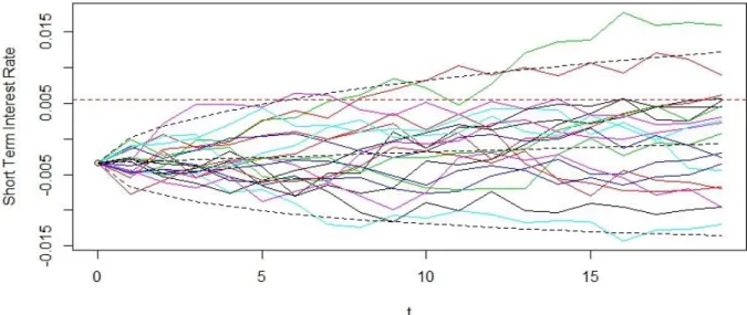
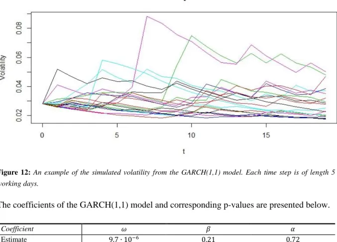
The third explanatory variable of interest is the market volatility, modelled through the standard GARCH(1,1) model on OMXS30. An example of 20 sample paths is shown in Figure 12.

(36)

33

Figure 12: An example of the simulated volatility from the GARCH(1,1) model. Each time step is of length 5

working days.

The coefficients of the GARCH(1,1) model and corresponding p-values are presented below.

Coefficient 𝜔 𝛽 𝛼

Estimate 9.7 ∙ 10−6 0.21 0.72

p-value 1.5 ∙ 10−5 3.4 ∙ 10−8 < 2 ∙ 10−16

To investigate the validity of the GARCH(1,1) model the residuals of the model are studied through a quantile-quantile-plot in Figure 13. In the figure data is on a daily basis. The left side of the graph exhibits non-normality, as expected due to the heavy left tail of the return distribution of equity indices presented by for example Z. Sheikh et. al. (Non-normality of Market Returns: A framework for asset allocation decision-making, 2009). Quantile-quantile plots for 5,10 and 21 day intervals exhibit the same type of patterns.

(37)

34

(38)

35

5. Results and Analysis

In this section the analysis carried out is presented and commented. First, the considered time intervals are investigated. Second, the results for the models utilised are presented in order to select the best model. Third, segmentation of the data by client attribute is analysed. Finally the proposed models are tested by using a one step ahead forecast to verify their validity.

5.1 Time Interval Analysis

One of the crucial factors for yielding accurate and meaningful forecasts is the choice of time interval between observations. In this section the results found when analysing different lengths of time intervals are presented. Furthermore, both overlapping and non-overlapping time intervals are analysed. The forecasts presented are produced from the ARIMAX model with the lowest AIC value. The graphs and out-of-sample performances for each model are compared and further analysed. The only exogenous variables in the ARIMAX model are monthly dummy variables, and results are presented only for segment A. However similar results are found for the other models and segments, including the fully aggregated deposits. Each model presented has been tested for robustness through a rolling window analysis.

By analysing the results for non-overlapping data, visualised in Figure 14-Figure 17, it is found that 5 and 10 days intervals give the most reasonable results. Models with 1 day intervals between data points suffer from short term fluctuations in the data yielding large standard errors and poor out-of-sample performances. 21 day intervals on the other hand results in too few observations and subsequently poor forecasts. The time interval analysis yield similar result for other models and further analysis on model selection is done in Section 5.2.

(39)

36

Figure 14: ARIMAX(1,1,1) model forecast for

segment A with 1 day time interval. MAPE of 9.9%.

segment A with 21 day time interval. MAPE of 14.2%.

The 21 day non-overlapping intervals produced inaccurate forecasts due to the few data points. To remedy this problem an alternative overlapping 21 day interval is considered. The overlapping interval time series analysis is modelled as a seasonal ARIMA (SARIMA) with the period 21 days. From Figure 18 a high degree of fluctuation can be seen as an effect of auto-correlation in the residuals. The apparent auto-auto-correlation of the residuals is shown in the ACF plot visualised in Figure 19. Further analysis on overlapping data is carried out separately in section 5.2.4.

(40)

37

Figure 18: SARIMAX(0,0,0)x(0,1,5)21 model forecast

for segment A with 1 day time interval. MAPE of 7.8%.

Figure 19: SARIMAX(0,0,0)x(0,1,5)21 model

residual ACF for segment A with 1day time interval.

Using 5 and 10 day intervals between observations seem most suitable for modelling deposit volume and will thus be further analysed throughout the result section, alongside overlapping 21 day interval data which will be analysed separately.

(41)

38

5.2 Model Selection

In this section the models presented in Section 3 are tested and compared, with the purpose of finding the most appropriate model for forecasting deposits.

5.2.1 Holt-Winters

The first model investigated is the Holt Winters model as presented in 3.1, which is a simple time series model appropriate for seasonal data. However, the deposit data used has proven to have too irregular nature to forecast with the help of Holt Winters model. Figure 20 shows the model fitted by using 90% of the data from segment A. The confidence intervals are wide and the MAPE indicates poor out-of-sample performance. The same pattern repeats itself for other segments and out-of-sample periods.

The seasonal pattern of a financial time series such as deposits for a relatively short time period is hard to translate into a working Holt Winters model. For monthly data on a longer time period one could perhaps expect the model to have higher predictive power. For example it is somewhat difficult to choose the periodicity of the model because of weekends and holidays.

(42)

39

5.2.2 Stochastic Factor Model

The stochastic factor model, as introduced in Section 4.4 for 5 and 10 day intervals are shown in Figure 21 and Figure 22. The model has low predictive powers, and this conclusion is also reached for other segments and out of sample periods. Including a time component does not significantly increase the predictive powers of the SF model. All coefficients for explanatory are very close to zero, except the one for the previous time periods’ deposit volume which is slightly below one.

Figure 21: SF model forecast for segment A with 5

day time interval. MAPE of 15.6%.

Figure 22: SF model forecast for segment A with 10

day time interval. MAPE of 9.9%.

Different from Castagna & Manenti (2013) an additional exogenous variable in the form of market volatility is added to the SF model used in hope to explain deposit volume behavior. However, attempts with only interest rates as the exogenous variables yield similar results. Thus a possible explanation for the differences in model performance between the studies can come from the data used. Castagna & Manenti (2013) use 13 years of public aggregated data for sight deposits in Italy, i.e. data on a highly aggregated level. A more thorough discussion on the data used and comparison to other studies will follow in the Discussion and Conclusion section.

5.2.3 ARIMA Models

In this section the results for the ARIMA models described in Section 3.3 are presented.

Plain ARIMA models do not include any explanatory variables, and cannot include seasonality. The model fits a deposit trend and for some out-of-sample period it exhibits a relatively good fit, as seen in Figure 23.