Known Roads
Real roads in simulated environments for the
virtual testing of new vehicle systems
www.vipsimulation.se
ViP publication 2015-2
Authors
Arne Nåbo, VTI
Carl Johan Andhill, Dynagraph
Björn Blissing, VTI
Mattias Hjort, VTI
Laban Källgren, VTI
ViP publication 2015-2
Known Roads
Real roads in simulated environments for the
virtual testing of new vehicle systems
Authors
Arne Nåbo, VTI
Carl Johan Andhill, Dynagraph
Björn Blissing, VTI
Mattias Hjort, VTI
Laban Källgren, VTI
Cover picture: Björn Blissing, Laban Källgren and Mattias Hjort, VTI Reg. No., VTI: 2012/0202-26
Preface
Known Roads is a collaborative project between Swedish National Road and Transport
Research Institute (VTI), Dynagraph, Volvo Trucks, Volvo Car Corporation and Swedish Road Marking Association (SVMF) within the ViP Driving Simulation Centre
(www.vipsimulation.se).
The scope of the project was to develop virtual representations of real roads to be used in driving simulators. These simulator roads can be used in studies where similarity between a simulator road and the real road is of benefit. Now, at the end of the project there are at least two following studies known that will use these roads.
At the start everything looked quite straight forward, ‘just measure the road and use existing available geographical data’. But, as often when working with real world data, there were quite a few hurdles to overcome. Geographical databases are not ideal and measurement data almost always contain errors that have to be removed in a gentle way. Different coordinate systems had to be harmonised etc. However, the enthusiastic researchers and engineers at VTI and
Dynagraph managed to find solutions to overcome these hurdles in a good way. Looking at the result we hope it will be useful for future simulator based research and system development. This report describes the work done and outline of the result. The main results though, are the virtual models, methods and tools developed.
The project has been financially supported by the competence centre ViP, i.e. by ViP partners and the Swedish Governmental Agency for Innovation Systems (VINNOVA).
The software developed in the project is available at the ViP common software platform ViPForge, https://www.vipforge.se/. Access is granted to ViP partners by the ViPForge administrator Jonas Andersson Hultgren at VTI (jonas.andersson.hultgren@vti.se).
Participants from VTI were Martin Fischer (who defined and initiated the project), Arne Nåbo (project manager), Laban Källgren, Björn Blissing, Mattias Hjort, Bruno Augusto, Thomas Lundberg and Peter Andrén (VTI consultant).
Participants from Dynagraph were Carl Johan Andhill and Richard Börjesson. Participants from Volvo Trucks were Peter Nilsson, Leo Laine and Niklas Fröjd. Participant from Volvo Cars was Mats Peterson.
Participant from SVMF was Göran Nilsson.
Gothenburg, October 2015 Arne Nåbo
ViP publication 2015-2
Quality review
Peer review was performed in September 2015 by Per Nordqvist, AB Volvo and Anders Bengtsson, HiQ. The authors have made alterations to the final manuscript of the report. The ViP Director Lena Nilsson examined and approved the report for publication on 6 November 2015.
Table of contents
Executive summary ...11
1. Introduction and problem description ...13
2. Project objectives...14
3. Method ...15
4. Result ...16
4.1. Road description based on map data and road measurements ...16
4.1.1. Road model in vehicle simulators – OpenDRIVETM ...16
4.1.2. Coordinate systems ...17
4.1.3. Coordinate transformations ...18
4.1.4. Data sources ...18
4.1.5. Methodology ...22
4.2. Road-related landscape description based on map data ...25
4.3. Creation of buildings based on map data ...25
4.3.1. Input ...25
4.3.2. Output ...25
4.4. Part-wise up-load of data ‘as you drive’ ...27
4.5. Integration of models in the simulator ...27
4.5.1. Simulation kernel ...27
4.5.2. OpenDRIVE™ ...27
4.5.3. OpenCRG and RSW ...28
4.5.4. Vehicle dynamic modelling ...28
4.5.5. Graphics broadcasting ...29
5. Discussion ...32
6. Conclusions ...34
7. Proposals and recommendation for an improved methodology of making simulator representations of real roads ...35
References ...37
Abbreviations
CORE Commander Of Road and Rail Environment FTS The Vehicle technology and simulation unit at VTI.
GPS Global Positioning System
G1 Curves sharing common tangent at joint points.
G2 Curves sharing common centre of curvature at joint point. Lantmäteriet The Swedish Agency for National Mapping
NVDB Nationell vägdatabas (National Road Database)
OpenCRG Open source project including a tool-suite for the creation, modification and evaluation of road surfaces, and an open file format specification CRG (Curved Regular Grid).
OpenDRIVE Open format specification to describe a road network's logic.
RST Road Surface Tester
RSW Road Short Wave
SIREN Simulator Sound Renderer
UDP User Datagram Protocol
ViP Driving Simulation Centre. A competence centre administered by VTI. VISIR Visual simulation of rail or road.
VTI Swedish National Road and Transport Research Institute
XML Extensible Markup Language
XPC target A real-time software environment from MathWorks.
2D Two-dimensional space
ViP publication 2015-2
List of figures
Figure 1. The roads included in “Known roads” are Road 40 Göteborg-Borås, Road 180
Borås-Alingsås, Road E20 Alingsås-Göteborg and the “Töllsjö” Road in-between these. The
plot in the figure shows the GPS data measured by the VTI RST vehicle. ... 13
Figure 2. VTI Road Surface Tester (RST) vehicle for measurement of road state. ... 18
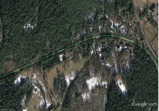
Figure 3. GPS measurements from the RST vehicle in two directions projected on a satellite
photo in Google Maps. ... 19
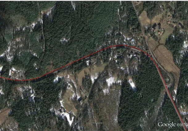
Figure 4. Road alignment according to NVDB on a satellite photo in Google Maps. ... 20
Figure 5. Google’s road direction of Road 180. ... 21
Figure 6. Lantmäteriets terrain data purchased along “Göteborgstriangeln” (the Gothenburg
Triangle, see also Figure 1). ... 22
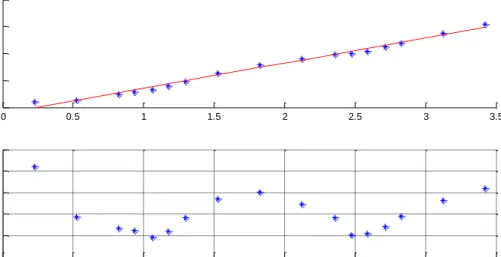
Figure 7. Top: Height of the individual laser tracks (blue) and the derived crossfall (red)
across the right lane for one longitudinal sample. Bottom: Height of the laser tracks after the
crossfall has been subtracted. All units on the scales are in metres. ... 23
Figure 8. A bird’s view of some buildings along “Known Roads”. ... 26
Figure 9. Picture of the generated road, terrain and buildings at Olskroken in Gothenburg. .. 29
Figure 10. Olskroken in Gothenburg. Map view in courtesy of Google Maps. ... 30
Figure 11. Picture of the generated road, terrain and buildings in Gothenburg. The green wall
is in reality a bridge whose height has been erroneously aggregated into the height data. ... 30
Figure 12. Photo of the true environment compared to the synthesized environment in Figure
11 (vantage point is approximately at the same world position). ... 31
Figure 13. Picture of Road 40 after refinement. The more or less manual treatments following
upon the automatic road generation consist of adding road embankment, vegetation, guard
rails and special objects. ... 31
List of tables
Table 1. Coordinate transformations between different systems. ... 18 Table 2. Measurements of the Road Surface Tester Vehicle. ... 19 Table 3. Classification and appearance of buildings and building heights as a function of their perimeter. Roofs are always black. Windows are added to the facades………...26
ViP publication 2015-2 11
Known Roads – Real roads in simulated environments for the virtual testing of new
vehicle systems
by Arne Nåbo1, Carl Johan Andhill2, Björn Blissing1, Mattias Hjort1 and Laban Källgren1
1 Swedish National Road and Transport Research Institute (VTI) 2 Dynagraph AB
Executive summary
The main aim of this project was to develop virtual representations of real roads for use in driving simulators. This was done in order to enable assessments of new systems on existing and well known roads in a driving simulator. This will increase the external validity of virtual testing. Furthermore, the usage of the virtual model of such roads makes the simulator results better comparable to earlier performed or later following road tests.
In order to ease the overall creation of virtual models of real roads as exactly as possible, and to enable the use of existing map data, there was a need to develop effective and efficient tools that can generate virtual road models more or less automatically from various data sources.
The roads connecting Göteborg-Borås-Alingsås-Göteborg were selected. The purpose for this is due to their proximity to the vehicle industry in west Sweden and to the test tracks “Hällered” and
“AstaZero”. However, the tools and methods developed can be used to build a virtual representation of any other road.
The project was carried out in steps, starting with data collection (investigation and assessment of available data) followed by data treatment (remove irrelevant data and errors, filtering, etc), modelling (mathematical description of road properties) and simulation (selection of data formats for real time simulation).
The description of the roadway through a landscape was broken into three main geometric parts: alignment (the route of the road in two-dimensional plane, described by clothoid splines), height profile (described by cubic splines) and cross-section (crossfall and banking, described by cubic splines). The road model format selected was OpenDRIVE, an open standard that stores road data
parametrically, and facilitates distribution and sharing of road databases amongst simulator facilities and software. It is also in use in the VTI simulators. For description of road surface unevenness, two formats were of interest; OpenCRG and RSW.
Data was collected from the following sources:
Road Surface Tester (RST), a vehicle for measurement of road properties (position, curvature, elevation, cross-fall, longitudinal profile).
National road database (NVDB). It contains a 2-dimensional description of the Swedish road network. Each road is defined by a number of points in the SWEREF 99 tm coordinate system.
Lantmäteriets terrain data. The data is a raster set which gives height above sea level (or rather the earth reference ellipsoid). The project used one raster 2x2 m in a corridor closest to the road, and one raster 50x50, for the landscape on greater distance from the road.
Lantmäteriets property map. It describes buildings in 2D polygons and their position. GSD- ortofoto. A satellite photo used for the description of the terrain surface.
12 ViP publication 2015-2 The generation of roads was then done in a stepwise process (model road sections – connect road sections – add road elevation – add crossfall – add road unevenness etc.).
The height and appearance of the buildings were created by a software tool that automatically generated 3D models using the 2D polygons.
Part-wise up-load of data ‘as you drive’ was facilitated by the VISIR graphics engine that is built upon OpenSceneGraph, which already supports streaming graphic databases from disk into memory. Learnings from the project are:
Although a lot of modelling could be done automatically, there was still quite some manual work in order to reach an overall representative simulator road, both regarding the road description and the graphics of the road environment.
It was found that the format OpenDRIVE tends to build up very large and complex databases and that it should be complemented by a format that better can handle open surfaces and complex road environments.
In this project an alternative way of describing road roughness, Road Short Wave (RSW), was developed. The benefits of the RSW format is its compact and analytic format.
Results from the project (tools and models) can be found at ViPForge (https://www.vipforge.se/login). For further information about project deliverables, see Appendix.
ViP publication 2015-2 13
1.
Introduction and problem description
Sweden is leading in the development of new safety functions for both trucks and cars. Also, the current development activities move constantly into the area of active safety and automation where assistance systems take over a part (e.g. lane keeping assistance, adaptive cruise control) or even all of the vehicle control tasks (e.g. automated driving, platooning). As a consequence, traditional test methods are difficult to apply (e.g. creating certain traffic conditions on a test track) or extremely dangerous (testing new functions in near crash or crash situations). Thus, the driving simulator turns more and more into an essential tool for testing and evaluating new active safety and driver assistance systems. In order to enable drivers to assess a new system in comparison to their experiences with car/truck driving, the best reference for them is to drive on an existing, well known road, in this case in a driving simulator. This is going to increase the external validity of the virtual testing a lot.
Furthermore, the usage of the virtual model of such a road makes the simulator results better comparable to earlier performed or later following road test.
To ease the overall creation of virtual models of real roads (to resemble their course, shape,
appearance and surroundings) as exactly as possible, and to enable the use of existing map data (height information, land use, location of buildings etc.), there was a need to develop effective and efficient tools that can generate virtual road models more or less automatically from different data sources. The purpose of selecting the roads connecting Göteborg-Borås-Alingsås-Göteborg (Figure 1) for generation in this project was their proximity to the vehicle industry in west Sweden and to the test tracks “Hällered” and “AstaZero”.
Figure 1. The roads included in “Known roads” are Road 40 Göteborg-Borås, Road 180 Borås-Alingsås, Road E20 Alingsås-Göteborg and the “Töllsjö” Road in-between these. The plot in the figure shows the GPS data measured by the VTI RST vehicle.
14 ViP publication 2015-2
2.
Project objectives
The project objectives were:
Eased generation of surrounding terrains for virtual roads based on map data.
Mathematical road description based on real geographical data and road measurement data. Part-wise upload of road and landscape descriptions in order to enable the use of long roads or
complex road networks.
Making the roads between Gothenburg, Borås and Alingsås, “Göteborgstriangeln” (the Gothenburg Triangle) and the “Töllsjö” Road available for driving simulator studies.
ViP publication 2015-2 15
3.
Method
As the project itself was defined as a “methodology” project, the detailed description of methods can be found in the chapters that follow. However, the project was set up as a step wise process, where each step had to be taken in order to fulfil the requirements of the following.
The main steps were: Data collection
Investigation of available databases containing information on road, terrain, land use and buildings. Purchase of selected databases.
Measurement of road properties and road appearance using the VTI RST vehicle (see chapter 4.1.4 and Figure 2 on page 18.
Data treatment
Remove irrelevant data from raw data. Remove errors, replace drop outs. Filtering of data.
Combine data from different databases to create a useful dataset. Modelling
Mathematical description of road properties. This is a data fitting process, and developing new tools for data fitting may be necessary in order to obtain usable mathematical descriptions of the datasets.
Simulation
Select data formats for models suited for real time simulations. Graphical and dynamical representation
Making the models perceivable in a driving simulator.
During the course of the project, it turned out that these steps could not be carried out entirely in sequence. Data treatment and modelling were generally carried out simultaneously, and we often had to go back a few steps and re-evaluate the developed methods.
16 ViP publication 2015-2
4.
Result
4.1.
Road description based on map data and road measurements
Geometric roadway design through a landscape can be broken down into three main parts: alignment, height profile and crossfall.
The alignment is the route of the road in a two-dimensional plane, which is assembled by straight lines, constant radius arcs and clothoids.
A clothoid (spiral) is a geometric primitive whose curve radius varies constantly over its length. It is also called transition curve as it is placed between straights and curves in order to avoid jerky driving. Mathematically the road’s curvature and its derivative are continuous functions and such a road alignment is G2 continuous. The inverted curve radius is called curvature, i.e. the curvature of a straight road is strictly zero as the radius is infinite.
The road’s macroscopic elevation follows the height profile of the underlying terrain (excluding tunnels and bridges).
At richer level of detail is the crossfall of the road. The purpose of the crossfall is water drainage and banking in order to accommodate driving in sharp curves.
At microscopic level one looks at the ruggedness of the road surface, e.g. bumps, pot holes, cracks and unevenness.
In this project we have used different data sources for generating a road model to be used in VTI’s driving simulators. The road model represents as accurately as possible an existing road where all the above levels of detail are combined. The general generating procedure is described in this report and the developed tools, mathematical algorithms and formulas necessary for the generation are described in detail in the “White Paper” by Hjort and Källgren (2015).
4.1.1. Road model in vehicle simulators – OpenDRIVETM
The road model used in the VTI vehicle simulators is OpenDRIVE1 which was developed by the company VIRES in Munich Germany. OpenDRIVE is an XML formatted open standard that stores road data parametrically, and facilitates distribution and sharing of road databases amongst simulator facilities and software.
The advantages of a parametric description are that road data can be analytically calculated which is fast and accurate, and that the database is fairly compact. The disadvantage is that the model is just an approximation of the real road, but by decreasing the error as much as possible without creating a cumbersome database one can re-create a road environment with high accuracy and realism. The road model alignment is described by clothoid splines, i.e. a series of connected straight lines, constant radius arcs and clothoids (lines and arcs can be regarded as special cases of clothoids). Elevation profile and crossfall are described by cubic splines, i.e. a series of third degree polynomials. When it comes to road surface roughness, there is no standard format in OpenDRIVE although you are allowed to append attachments of any format in order to describe the road surface. Two formats for road surfaces are implemented at VTI, OpenCRG and RSW.
1 http://www.opendrive.org/
ViP publication 2015-2 17 OpenCRG
OpenCRG2, where CRG stands for Curved Regular Grid, is a complementary project to OpenDRIVE
and is developed by German car companies. Principally CRG is a raster data set that describes the road surface’s vertical deviation from a plane surface. The advantage of CRG is the high accuracy, but one drawback is extremely large datasets (order of 300MB).
RSW
RSW stands for Road Short Wave, and is a format that was developed at FTS/VTI for the ViP project Known Roads. RSW is, contrary to OpenCRG (but in analogy with OpenDRIVE), a parametric data format where road surface deviation is described by cubic splines in longitudinal tracks. Each track is independent from the others, and look up of the deviation from a virtually plane surface at any point of the road is analytically calculated with e.g. bilinear interpolation.
When approximating the road surface with cubic polynomials, high-frequency road noise is removed. Hence the name “Road Short Wave”; it is rather the short wave information of the road in order of 1 m that describes the road surface. Of course the accuracy of the model can be varied, and higher
frequencies reproduced, but that is a trade off with the database size. OpenCRG (described above) is preferred if an unspoiled data set is desired.
4.1.2. Coordinate systems
In order to describe a geographical position or direction on the road or in the road surroundings, there are standard sets of coordinate systems to choose from.
WGS84 – GPS
WGS843 stands for World Geodetic System 1984 and is a global geodetic reference system. WGS84 is
used as coordinate system for the GPS technology. Principally a position’s coordinates are given in latitude, longitude (degrees) and height above the reference ellipsoid.
SWEREF 99 tm
SWEREF 99 tm4 is a coordinate system used for geographical positions in Sweden. It is a Cartesian
coordinate system that locally gives linear and fast calculations with small geographic error. SRH
The SRH system is a road following, non-linearly varying coordinate system which is well suited for describing position along a road.
The S-coordinate gives the distance along the road’s chord line from its start (s = 0). The S-axis is always tangential towards the road’s chord line. The R-axis is perpendicular to the S-axis and describes the position’s deviation from the road centre chord line. Positive values of R lay on the left side of the road with respect to the to the S-axis. H is height above road plane at the centre chord line. The unit of all three axes is meter.
The SRH coordinate system varies along the road’s chord line when the road bends, as the S-axis always points along the roads tangential direction. However, the H-axis direction always points upwards despite any banking of the road in the SR-plane.
2 http://www.opencrg.org/
3 http://sv.wikipedia.org/wiki/WGS84
18 ViP publication 2015-2 4.1.3. Coordinate transformations
Table 1 lists the algorithms that perform coordinate transformations between the different coordinate systems.
Table 1. Coordinate transformations between different systems. Coordinate
system
WGS84 SWEREF 99 tm SRH local xyz
WGS84 - PROJ.4
SWEREF 99 tm PROJ.4 - 𝑥 = 𝑥̅ cos 𝛼 − 𝑦̅ sin 𝛼
𝑦 = 𝑥̅ sin 𝛼 + 𝑦̅ cos 𝛼
SRH Line, Circle,
Fresnel integral -
local xyz 𝑥 = 𝑥̅ cos 𝛼 − 𝑦̅ sin 𝛼
𝑦 = 𝑥̅ sin 𝛼 + 𝑦̅ cos 𝛼
Lidström’s algorithm -
PROJ.45 is an open source project for cartographic projections and transformation between different
reference systems. Transformation from road following coordinate system SRH to global SWEREF 99 tm system is analytic. Depending on the road’s local alignment (straight, arc or clothoid) the XY-position is calculated either with linear transformation, calculations of circle or with help from Fresnel integrals, respectively.
In order to convert a position from XY-system to road following SRH is non-trivial, and in some cases there are ambiguous solutions (e.g. where roads cross). The conversion can be made analytically for straight lines and arcs, but for clothoids an iterative algorithm must take place.
4.1.4. Data sources RST
Figure 2. VTI Road Surface Tester (RST) vehicle for measurement of road state.
5 http://trac.osgeo.org/proj/
ViP publication 2015-2 19 The Road Surface Tester (RST)6, shown in Figure 2, is VTI’s testing vehicle for measurement of road
state. The data listed in Table 2 was recorded by RST and used for the generation of virtual roads. Table 2. Measurements of the Road Surface Tester Vehicle.
Variable Method Unit Sampling distance
Position GPS WGS84 (lat – long)
[°] ≈20 m
Curvature Gyro [1/m] 0.1 m
Elevation Attitude angle [m] 0.1 m
Crossfall Inclinometer [m] 0.1 m
Longitudinal profile Laser rod, 17-19
tracks [m] 0.1 m
A two-lane road is first measured in one direction and then in the other direction in order to get data of the complete road surface.
The position is measured with a GPS approximately each 20th meter and the accuracy is ± 10m. As
shown in Figure 3 the measurements do not follow the road as desired. The reason may be trees occluding the GPS satellites or system drifting.
Figure 3. GPS measurements from the RST vehicle in two directions projected on a satellite photo in Google Maps.
20 ViP publication 2015-2 For the road unevenness modelling data from 17 parallel longitudinal tracks, measured with the RST lasers, are used.
The measurement width with 17 lasers is 3.2 meters, while 19 lasers span 3.65 meters. The two outer lasers are mounted at an angle outwards to allow for measurements outside the width of the laser bar. However, using all 19 lasers would give us measurements outside the road edge hence measurements by the two outer lasers (left/right) are not used in the modelling. For narrow roads a smaller number of laser tracks are used for measuring each lane, i.e. in the collection of data from the “Töllsjö” Road only 15 laser tracks per lane are used.
The lasers measure the distance to the ground at a high frequency (16 or 32 kHz depending on laser type), which at a vehicle speed of 90 km/h results in one measurement value every 0.08 or 0.15 mm. Data is however not stored at that frequency. Instead a mean value from each laser is stored every 10 cm. It is possible to sample data at a shorter interval than that if needed.
Other signals are measured each decimetre and with high accuracy. NVDB
The National road database (NVDB) 7 contains a 2-dimensional description of the Swedish road
network. Each road is defined by a number of points in the SWEREF 99 tm coordinate system (described on page 17 above). The points lay unevenly spread along the road centre chord line, and long straights can be described with a few points while curvy parts naturally need more points. This way of representing a road opens up for a natural conversion to clothoid splines.
From our point of view NVDB is the (most) correct data source for location of the road’s world position. Deviation from Google Maps (Figure 4) can be explained by skewing errors in Google map projections. Even Google’s own road alignment lays off-road compared to satellite photos in Google Maps.
Figure 4. Road alignment according to NVDB on a satellite photo in Google Maps.
ViP publication 2015-2 21 Google
Google can also be used in order to find a road’s alignment in the world, by making a travel direction request between the ends of the road either in Google Maps or Google Earth (Figure 5). The direction can be exported to a kml-file (xml format) in order to be parsed in any software. The coordinates are GPS points in the WGS84 system.
The Google data set is as the data in NVDB non-uniformly sampled, i.e. relatively few data points constitute the road path accurate enough. However, we have seen examples where Google direction deviates from true alignment (according to NVDB).
Figure 5. Google’s road direction of Road 180.
Lantmäteriets terrain data
Lantmäteriet8 delivers the height data of the terrain at macroscopic level (Figure 6). The data is a raster
set which gives height above sea level (or possibly the earth reference ellipsoid). In this project there are two levels of detail to use, one 2x2 m raster in a corridor closest to the road, and one 50x50 m raster for the landscape at greater distance from the road.
The format is ordinary text files where terrain height data is divided into tiles, and where each tile has the raster matrix.
8 http://www.lantmateriet.se/
22 ViP publication 2015-2 Figure 6. Lantmäteriets terrain data purchased along “Göteborgstriangeln” (the Gothenburg
Triangle, see also Figure 1).
4.1.5. Methodology
In this chapter the method developed to convert measured source data to a simulated road and a road environment is briefly described. A more detailed description is presented in the “White Paper” by Hjort and Källgren (2015).
The aim was to automatize the converting process as much as possible, but it is inevitable that some parts demand manual processing and inspection of data.
The following five steps describe the process:
1. The road is measured in both directions using the RST vehicle.
2. Road description from NVDB and terrain height data from Lantmäteriet are acquired. 3. Using NVDB coordinates description, clothoid spline fittings are carried out for as long road
sections as possible using the Cornucopia algorithm which converts handwritten curves into a spline of clothoids (Baran, Lehtinen and Popovic, 2010). This algorithm produces a
2-dimensional description of a road section using straight road segments, circle segments and clothoid segments as building blocks. Moreover, the result is G2 continuous, meaning that the tangent vector and the curvature are continuous along the road. This is very important for a satisfying visualization and smooth motion cueing.
4. The road sections need to be connected. There is often a need to connect two sections that have a gap between them. Then in-house developed methods are used to find a connection that is G2 continuous.
ViP publication 2015-2 23 5. The road elevation (or height) is determined. It is not possible to use RST elevation data only,
due to sensor drifting. Instead, we use the Lantmäteriet terrain height data and interpolate the height at the middle of the constructed 2-D road (sampled with 0.1 m steps). The interpolated elevation data needs to be adjusted by hand to remove influences from dips or peaks in the surrounding terrain (most likely present due to pre-filtering of the terrain data by
Lantmäteriet). The elevation data then needs to be low-pass filtered. Finally, elevation variations of higher frequencies can be added using high-pass filtered RST elevation data. A spline fit of 3rd degree polynomials of the elevation is performed since that is the elevation
format in OpenDRIVE. The difference between the re-generated elevation from the splines and the desired elevation is stored.
The road elevation of the centre line is thus determined from adding the terrain generated elevation (low frequency) and the RST elevation data (high frequency). The general road surface elevation can then be described as a grid, by adding the elevation of the centre line to the grid from the laser elevation measurements. This is the complete road elevation as determined from the measurements, and which we aim to re-create in the simulator.
Following the OpenDRIVE standard, the elevation information needs to be divided into separate parts, which when added together should result in the original elevation grid.
These parts are:
I. Elevation of the road centre (described by a spline of 3rd degree polynomials).
II. Crossfall of each lane, i.e.an angle which continuously change along the road, and which is also described by a spline of 3rd degree polynomials.
III. Local deviations of the road surface elevation described by a grid, or raster, of data points, which are denoted CRG data.
Ideally, the average of the CRG data points should be zero. However, as illustrated in Figure 7, there is often an underlying pattern of the laser tracks after removing crossfall from the measurements. Thus, it makes sense to create a sub-layer of elevation information for each longitudinal laser track. This can be done using 3rd degree polynomial splines, just as for the road centre elevation. These splines, one
for each measured laser track, are denoted RSW (Road Short Wave). What is left of the laser grid elevation after removing the RSW elevation is stored in the CRG data grid file.
Figure 7. Top: Height of the individual laser tracks (blue) and the derived crossfall (red) across the right lane for one longitudinal sample. Bottom: Height of the laser tracks after the crossfall has been subtracted. All units on the scales are in metres.
0 0.5 1 1.5 2 2.5 3 3.5 0 0.05 0.1 0.15 0.2 0 0.5 1 1.5 2 2.5 3 3.5 -0.01 -0.005 0 0.005 0.01 0.015
24 ViP publication 2015-2 The road normally consists of two lanes, measured in each direction. The measurements are first adjusted so that they use the same longitudinal data. After that the unevenness and crossfall information of each lane is evaluated separately before eventually being assembled into a one road description.
The following steps describe that process:
1. The longitudinal distance information from each lane measurement needs to be transformed to represent the centre of the road. Due to the difference in length between the inner and outer track of a curve, the two lane measurements may differ in total length. The scaling of the longitudinal distances is done in two steps:
a. Re-scaling the distance information (continuously) of the left lane so that it matches that of the right lane.
b. Re-scaling the distance information (continuously) of the two lanes so that it matches the distance of the cornucopia generated road
For the first step, the longitudinal profile of the first laser track (the one to the very left side of the laser bar) is used. It should represent the unevenness of the road centre for both
measurements, i.e. they should ideally be identical. This is however most often not the case due to a couple of problems that can occur during measurements. For example, road works can force the RST vehicle over into the opposing lane. On sections with traffic islands or other parts where the road lanes are a distance apart, there will of course be no matching. Such discrepancies need to be manually addressed. Then, to make a matching feasible, the road distance of one of the lanes needs to be continuously stretched or compressed in order to match the other lane. An algorithm for this was developed using the road curvature as a measure. It will, however, not result in a perfect match along the road. A possibility for a better matching algorithm could be based on the Dynamic Time Warping algorithm.
The second step uses the RST curvature of the right lane, which is scaled against the curvature of the 2D description of the road (clothoid description from NVDB data) in order to align the two data sets. The same algorithm as for the first step is used for the scaling.
2. From measured crossfall values, a crossfall angle is determined, which is then stored in OpenDRIVE format as a spline of 3rd degree polynomials. The difference between the
re-generated crossfall splines and the measurement data is added to the longitudinal profile data. In addition, the difference between the re-generated elevation from the splines and the desired elevation is also added.
3. The resulting longitudinal track data can either be represented directly by using the OpenCRG format. If the amplitude of the data is too large it could however be useful to represent short wave variations of the data as separate polynomial splines. A G1 continuous spline fitting is then performed and stored and can be used as a VTI extension of the OpenDRIVE format. The discrepancy between the longitudinal track data and the re-generated data from the splines is then stored as a CRG file. Depending on the settings used in the spline fitting process, the minimum wavelength of polynomial splines can be chosen. Choosing a short enough wavelength will result in a CRG file containing practically white noise only.
4. Currently, the unevenness of the road cannot not be visualised in the driving simulator using standard triangulation techniques with corresponding lighting calculations. Instead, in order to visually detect uneven spots, the longitudinal track height information was used as a base for calculating shadows which are then superimposed on the road surface textures. Although far from state of the art lighting techniques, it may present the driver with information about the road unevenness.
ViP publication 2015-2 25
4.2.
Road-related landscape description based on map data
Terrain data such as elevation, ground usage and satellite imagery was purchased from Lantmäteriet (GSD- terrain data, vector, GSD- height data, grid 2+, GSD- height data, grid 50+, GSD- ortofoto, colour, 0.5 m) and processed into a three dimensional database using Virtual Planet Builder9. This tool
generates a graphics database that contains several levels of detail. However, shapes like bridges and overpasses must be processed before converting them to the database, otherwise their height would show up as a wall across the road (see Figure 11). Using the road elevation from the previous step, the elevation data is adjusted to a level representing the entire road. This also reduces the possibility of Z-fighting10 when applying the road geometry later.
4.3.
Creation of buildings based on map data
To increase the realism of the driving environment it was decided to re-create all the buildings along the roads. This is a huge challenge since there are about 32000 buildings in a 1-kilometre-wide corridor along the roads.
In order to re-create the buildings some kind of map or drawing to start with was needed. The area is too big and the buildings are too many to try to do the mapping ourselves (from scratch). Fortunately, Lantmäteriet keeps digital maps of all Swedish buildings. The maps are in the open Esri shape file format where every building is represented by a 2D polygon.
There are different solutions for making a 3D model of a building from a 2D polygon description: 1. Using existing software like 3D Studio Max in a semi-automated manor. In this case time
would be spent to manually model parts of the buildings.
2. Write a software tool which automatically generates 3D buildings from the 2D polygons. It was decided to go for the latter solution since that will save time in future projects and increase the value of the ViP platform. The software tool is called “map2building”.
4.3.1. Input
The input to the software tool is the map with 2D polygons from Lantmäteriet (GSD- buildings map, ground coordinates). This map is in the SWEREF 99 TM coordinate system. It is noticeable that in this coordinate system Gothenburg is located at x = 326000 and y = 6403000. In some cases, location of the 3D models this far from the origin is not wanted since it will decrease the floating point precision. To save computing time when dealing with this many 3D objects, the solution is to stick to limited number of value figures that are better used for decimals. Thus, the program offers the possibility to offset the buildings, moving them closer to the origin.
4.3.2. Output
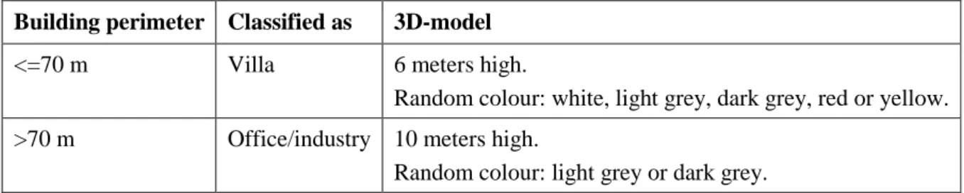
The software tool reads each 2D polygon and generates a 3D volume. As there is no information about building height and type on the building map, it was decided to estimate this in relation to the
perimeter of the building (Table 3, Figure 8).
9 http://www.openscenegraph.org/index.php/documentation/tools/virtual-planet-builder 10 http://en.wikipedia.org/wiki/Z-fighting
26 ViP publication 2015-2 Table 3. Classification and appearance of buildings and building heights as a function of their
perimeter. Roofs are always black. Windows are added to the facades. Building perimeter Classified as 3D-model
<=70 m Villa 6 meters high.
Random colour: white, light grey, dark grey, red or yellow. >70 m Office/industry 10 meters high.
Random colour: light grey or dark grey.
Figure 8. A bird’s view of some buildings along “Known Roads”.
The software tool can output the 3D models in these formats: osgt
3ds ive osgb
When driving in large areas you typically cannot see the entire 3D world in every single moment. As an example, for computing reasons there is no need to display Gothenburg buildings when driving through Borås. The 3D engine, VISIR11, has functionality to stream 3D models in and out based on the
position of the driver. To simplify this work, the software tool (map2building) can group buildings into chunks where buildings in the same area will be included in the same file. As an example,
map2building can “be told” to group buildings into areas having a side of 2000 meters. The output will
ViP publication 2015-2 27 be that buildings are divided into about 130 different files (like the squares of a chessboard). VISIR will then show only the files that are relevant with respect to the driver's position.
4.4.
Part-wise up-load of data ‘as you drive’
The VISIR graphics engine is built upon OpenSceneGraph12, which already supports streaming
graphic databases from disk into memory. It is reading the parts of the database that are visible at the moment and paging out parts of the database that are no longer in use. But the databases have to be prepared so that they include information about how the level of details should be loaded. This is done as a pre-processing step.
There are also hardware issues to consider since the databases contain a massive amount of data. This puts though requirements on network bandwidth and hard drives. To facilitate this a high performance file server was purchased and integrated into the simulator using dual network connectors, resulting in a 2 Gbit/s connection.
4.5.
Integration of models in the simulator
4.5.1. Simulation kernel
The vehicle simulation is driven by the simulation CORE13, which can be viewed upon as the logic
layer of the simulation.
CORE’s main responsibilities are:
Routing data between internal modules.
Routing data between peripheral programs via e.g. Ethernet. Supervising scenario and events during drive.
Recording experimental data.
The CORE is an abstract layer and a simulation kernel application is built on top of CORE. For this project the “vsim12” road vehicle simulation kernel14 was used.
4.5.2. OpenDRIVE™
“OpenDRIVE™ is an open file format for the logical description of road networks. It was developed and is being maintained by a team of simulation professionals with large support from the simulation industry. Its first public appearance was on January 31, 2006.”15
VTI/FTS decided at an early stage to support OpenDRIVE and use the format as the standard road description in vehicle simulation. Since 2010 VTI is a member of the OpenDRIVE core team.
Basically an OpenDRIVE database is a hierarchical description of roads in a road network, where each road has geometrical properties like prolongation of chord line, slope and crossfall. Moreover,
OpenDRIVE describes the lane system of each road and how roads are connected to each other in the road network. (The specification can be downloaded from the OpenDRIVE webpage.)
12 http://www.openscenegraph.org/
13 Commander Of Road and Rail Environment - owned by ViP. 14 Developed by FTS at VTI.
28 ViP publication 2015-2 In order to read and make use of an OpenDRIVE database in simulation runtime, an interface has been developed at VTI and can be downloaded from the ViPForge16.
The OpenDRIVE database is used in the simulation kernel for logical look ups like; where is the car? where can the autonomous vehicle go? which is the slope of this hill? It is also read by the graphics engine VISIR in order to visualize the road network (Bolling et.al., 2013), and by SIREN17 (Andersson
and Genell, 2013) in order to give sound cues to the driver from surrounding traffic.
One of the main objectives of this project was to convert geographical data sources like road position GPS measurements, terrain height and road unevenness into OpenDRIVE format, in order to
reproduce the road environment as authentically as possible in a simulator. (For further reading of such methods see chapter 4.1 Road description based on map data and road measurements). 4.5.3. OpenCRG and RSW
In order to simulate road unevenness two formats have been evaluated in the ViP project
KnownRoads; OpenCRG and RSW. Road unevenness is an important matter when it comes to vehicle dynamics and tire simulation.
OpenCRG18 is an open file format suitable for “detailed description, creation and evaluation of road
surfaces” and was developed in collaboration with the OpenDRIVE format. CRG stands for Curved Regular Grid and is a z deviation raster from a plain road surface. There are free libraries available for downloading in order to make use of such data sets in simulation software.
During this project an alternative data format was presented, called RSW for Road Short Wave. Rather than make use of all the road unevenness measurements, a parameterized curve format (cubic splines) is used in order to reproduce road unevenness. Fitting curves to a high frequency data set results in some data loss, hence the name Road Short Wave (meaning that the very highest frequencies are lost). However, lost frequencies are presented as visual cues even though they can never be felt in the motion system.
The advantage of OpenCRG is that high accuracy simulation can be performed, but the data sets can be quite large, even impossible to use in primary memory. The advantage of RSW is the compact parameterized format, but some data loss is to expect. Depending on specific project objectives, one of the formats is selected in relation to the desired level of authenticity.
Both formats are supported by the VTI simulation kernel, and the data interfaces and look up algorithms are integrated into the VTI Common Libraries (see foot note 16).
4.5.4. Vehicle dynamic modelling
In order to be able to drive around in the simulated road network a vehicle model responds to driver input (throttle, steering wheel), calculates forces and returns kinetic information to the simulation kernel. The simulation kernel makes use of that information, i.e. calculates position on the road, routes accelerations to any motion system and force feedback to the driver steering wheel etc.
Any vehicle model can be used, either integrated in the simulation kernel binary or as external software. In this project an advanced external truck model was running on an XPC target, communicating with the simulation kernel via UDP on Ethernet.
16 libvtiopendrive is a part of VTI Common Libraries - https://www.vipforge.se/projects/libvti. 17 SIREN is the audio engine owned by ViP.
ViP publication 2015-2 29 During runtime, the simulation kernel looks up road information at the current vehicle position from the road database, e.g. curvature, slope and road roughness. Radial forces due to curvature and g-forces due to slope are sent to the vehicle model for further calculations. Road unevenness information is fed to each tire of the vehicle model, which in turn can produce tire forces and vibrations in the model.
4.5.5. Graphics broadcasting
The world position and orientation of the vehicle are calculated (in the simulation kernel) from its current position in the road network and then sent to the graphics engine. Making sure that the graphics engine uses the same underlying road database, the visual cueing is coherent with the dynamic sensation of the drive.
One important factor is that road damages and pot holes should be accurately presented to the driver in the graphics and fed to the vehicle dynamics for the motion sensation. This is a matter of
synchronization of two cues, visual and motion.
When using road surface measurement data, the road damages must be accurately modelled in the OpenCRG or RSW format and also displayed in the graphics with help of displacement or bump mapping. As stated previously (see chapter 4.5.3 OpenCRG and RSW) one should be aware that the RSW format loses high frequency information.
Another problem to solve is the time delays; there are different time delays between kernel, graphics and projectors, and between kernel, dynamics and motion. This could end up in a scenario where the sensation of the pot hole is somewhere else than where the driver expects it to be from the visual cue.
30 ViP publication 2015-2 Figure 10. Olskroken in Gothenburg. Map view in courtesy of Google Maps.
Figure 11. Picture of the generated road, terrain and buildings in Gothenburg. The green wall is in reality a bridge whose height has been erroneously aggregated into the height data.
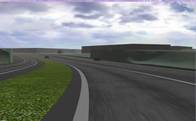
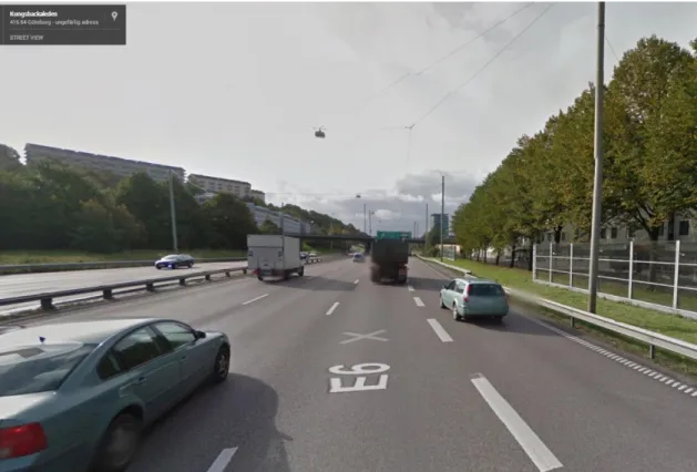
ViP publication 2015-2 31 Figure 12. Photo of the true environment compared to the synthesized environment in Figure 11 (vantage point is approximately at the same world position).
Figure 13. Picture of Road 40 after refinement. The more or less manual treatments following upon the automatic road generation consist of adding road embankment, vegetation, guard rails and special objects.
32 ViP publication 2015-2
5.
Discussion
At the start of the project the question “What is a good simulator road?” was discussed. The answer was found not to be straightforward. High realism in simulation requires detailed models, and that means big data sets, while performance in real time simulations requires reduced data sets. Thus, there are built-in conflicting objectives. This means you have to prioritize the things that are of importance for the actual simulation, i.e. the parameters and the level of detail you want to study and evaluate. For example, if vehicle stability is in focus the description of the road and road surface should be detailed and less effort made on the rest of the road environment, but if traffic sign design is important, more effort should be put on the graphics of these, etc.
After having discussed this question for a while, the project team decided to characterize a good virtual representation of a real road by these two sentences;
The driver shall be able to experience familiarity with the real road. The vehicle model shall behave similar to a real vehicle on the real road.
An ambition at the start of the project was to use data from different data sources and then, by creating a ‘tool’, generate simulator roads automatically. This ‘tool’ turned out to become more of a method, consisting of a number of steps where data had to be treated and manually checked and corrected in each step. However, within each step it was possible to use tools, or routines, to ease the workload. One reason for having to check between steps is that data sets are not flawless. Data can be missing, erroneous or old by a number of reasons. This was the case for data from both the RST vehicle and the geographical databases. If using the data without checking, the simulator road will not be correct. Depending on the quality of the data sets, checking and correcting can be more or less demanding. Ideally, a tool that combines all the developed methods would facilitate the process of generating a simulator road. Although not straightforward, creating such a tool should be something to aim for. Finally, the last project objective was to make the roads between Gothenburg, Borås and Alingsås available for driving simulator studies. The included roads were modelled in a rudimentary level of detail in this project (except for some shorter road segments). The reason for this was that it must be the actual following projects that use “Known Roads” that set the requirements on what should be highlighted, and the work to do this has to be included in those projects.
So far, the roads generated in this project have been used and enhanced as follows:
Road E20/E6 through Gothenburg, in the ViP project AP7: DB2 - Driver and system heavy vehicle steering19 (report in progress).
Road 180 from Borås to Alingsås, in the ViP project MT11: High speed Control20
(report in progress).
Road 40 between Gothenburg and Borås, in the ViP associated project Electric Road Systems in Driving Simulator (Nåbo et al., 2015) sponsored by the Swedish Energy Agency.
In addition, Road 180 from Borås to Alingsås has been used in collaboration with Volvo Trucks for evaluating truck cabin vibrations due to uneven road. A work that was presented at the International Symposium on Heavy Vehicle Transportation Technology (Hjort el al., 2014).
19 http://www.vipsimulation.se/default.asp?page=ap7:-db2---driver-and-system-heavy-vehicle-steering&pid=270 20 http://www.vipsimulation.se/default.asp?page=mt11:-high-speed-control&pid=297
ViP publication 2015-2 33 Road 40 between Gothenburg and Borås is probably unique in length for a simulator road as it
represents about 60 km of a real road.
Thus, the “Known Roads” seems to be attractive for simulator studies and we hope that the methods, tools and roads will be used and appreciated in driving simulator studies in the future.
34 ViP publication 2015-2
6.
Conclusions
Tools and algorithms have been developed for merging different data sources into one realistic and authentic virtual road model for simulation purposes.
NVDB is our first choice of road network coordinates.
Road environment virtualization ranges from microscopic level (road unevenness) to macroscopic level (road world alignment).
For rural roads and simpler city environments the developed tool can generate OpenDRIVE files that describe the roads. However, for large databases and complex road environments OpenDRIVE may be cumbersome and a different solution may be needed.
Add-ons have been made to the OpenDRIVE standard in order to simulate an uneven road. Lantmäteriet holds the necessary maps for generating 3D buildings along most Swedish roads. It was fairly easy to write a software tool which could generate the 3D buildings.
To make use of VISIR's streaming capacity, buildings had to be grouped into geographical chunks.
The classification and correctness of the buildings can be further improved by making use of additional maps showing for example land use.
It would be possible to add more details and realism to the buildings. It is the current simulator's 3D graphics hardware that sets the limit.
ViP publication 2015-2 35
7.
Proposals and recommendation for an improved methodology of
making simulator representations of real roads
OpenDRIVE (see chapter 4.5.2 OpenDRIVE™) has the past years been the standard way of describing road networks in the VTI simulators’ virtual environments. However, one may ask if the format is optimal and can solve the problem of describing any kind of road environment. When it comes to simple road networks as for example rural roads, standard highway exits or four-way crossings OpenDRIVE format is feasible.
In this project it was noticed that for very complex road networks, such as the one along Road E6 in Gothenburg with many exit and entry roads and changes in lane system, OpenDRIVE tends to build up very large and complex databases in order to describe junctions logically. A junction is basically a choice of route between many connecting roads. Roundabouts and other open surfaces or crossings cannot easily be represented by OpenDRIVE format, which is a strict road following system.
Moreover, OpenDRIVE is a very gabby format, where data may be duplicated and implicit values are explicitly stated, which in the end give larger databases than needed.
Based on the work in the reported Known Roads project we draw the conclusion that OpenDRIVE would benefit from a complementary format that can handle open surfaces and complex road environments and be more implicit in its way of handling data. For example, we know that roads are connected with preserved angles and curvatures, so those data are implied by previous road segments. Moreover, the OpenDRIVE database is used for different purposes:
In the visualization engine, where the road is visualized.
In the simulation kernel, logical look ups are used for traffic modelling, vehicle dynamics and motion queuing.
For complex road networks, it is the latter that becomes very problematic and in many cases
impossible. With a complementary format, the logical choice of route through the road network can be handled differently than with OpenDRIVE; by putting choice of road at lane level, e.g. autonomous traffic can be simulated in a more realistic fashion, and connecting the network is less cumbersome. In the Known Roads project an alternative way of describing road roughness, Road Short Wave, was developed (see chapter 4.5.3 OpenCRG and RSW). The benefits of the RSW format is its compact and analytic format, which is feasible for large road databases.
The software tool map2building can be improved as follows:
Currently the buildings are located at z = 0. Positioning of the buildings on the right altitude has to be done by VISIR. A future improvement of map2building would be to read the terrain, or the elevation data used to create the terrain, to give the buildings the right altitude from start.
Currently we classify building types based on their perimeter length. There are other data sets that could help in doing this classification. By reading other maps, which include ”land use type”, buildings can be classified as industrial, office, residential, farm etc.
ViP publication 2015-2 37
References
Andersson, A. and Genell, A. (2013). SIREN – Sound Generation for Vehicle Simulation. ViP publication 2013-3. Linköping, Sweden: Swedish National Road and Transport Research Institute (VTI).
Baran, I., Lethinen, J. and Popovic, J. (2010). Sketching Clothoid Splines Using Shortest Paths. Computer Graphics Forum, Volume 29, Issue 2, pp. 655–664.
Bolling, A., Lidström, M., Hjort, M., Nordmark, S., Sehammar, H., Sjögren, L., et al. (2013). Improving the realism in the VTI driving simulators. VTI rapport 744A. Linköping, Sweden: Swedish National Road and Transport Research Institute (VTI).
Hjort, M., Källgren, L., Augusto, B. and Fröjd, N. (2014). Evaluation of truck cabin vibration by the use of a driving simulator. Proceeding of the International Symposium on Heavy Vehicle Transport Technology – HVTT13, 27-31 October, 2014, San Luis, Argentina.
Hjort, M. and Källgren, L. (2015). A method for road description based on map data and road
measurements (“White Paper”). ViP PM 2015-2. Linköping, Sweden: Swedish National Road and Transport Research Institute (VTI).
Nåbo, A., Börjesson, C., Eriksson, G., Genell, A., Hjälmdahl, M., Holmén, L., Mårdh, S. and Thorslund, B. (2015). Electric Road Systems in Driving Simulator. Design, test, evaluation and demonstration of electric road systems and electric vehicles by using virtual methods. VTI rapport 854. Linköping, Sweden: LiU-Tryck.
ViP publication 2015-2 39
Appendix - List of project deliverables and materials
ViP Project: MT10 ViP – Known Roads.
No Title/Description Responsible Format Storage Class
1
Known Roads – Real roads in simulated environments for the virtual testing of new
vehicle systems Arne Nåbo
ViP
Publication ViP home
page Public 2 ViP - Known Roads Final report Arne Nåbo
ViP Report (adm) ViP manager ViP internal 3 RST data (data from the VTI RST vehicle) Mattias Hjort Database
VTI server
VTI internal
4
A method for road description based on map
data and road measurements (“White Paper”) Mattias Hjort
Report /
Manual ViPForge ViP internal 5
A software for generating buildings based on map data Carl Johan Andhill Report / Manual ViPForge ViP internal 6
SW tool for generating buildings based on map data
Carl Johan
Andhill SW tool ViPForge ViP internal 7 Landmarks (buildings, bridges, etc.)
Carl Johan
Andhill Database ViPForge ViP internal
8
"Göteborgstriangeln" (the Gothenburg
Triangle) road description Laban Källgren Database ViPForge ViP internal 9
"Göteborgstriangeln" (the Gothenburg
Triangle) terrain description Björn Blissing Database ViPForge ViP internal 10
"Göteborgstriangeln" (the Gothenburg Triangle) landmarks
Carl Johan
Andhill Database ViPForge ViP internal 11 GSD- ortofoto, 48 pcs Björn Blissing Tiff
VTI server
VTI internal 12
GSD- fastighetskartans byggnader, vektor 165
km2 Björn Blissing Shape VTI server VTI internal 13
GSD- geodata, "Göteborgstriangeln" (the
Gothenburg Triangle) Björn Blissing Database VTI server
VTI internal
14 File server Björn Blissing PC
VTI Sim III
VTI internal
40 ViP publication 2015-2 Contact list:
Carl Johan Andhill, Dynagraph (can@dynagraph.se) Björn Blissing, VTI (bjorn.blissing@vti.se)
Mattias Hjort, VTI (mattias.hjort@vti.se) Laban Källgren, VTI (laban.kallgren@vti.se) Arne Nåbo, VTI (arne.nabo@vti.se)
www.vipsimulation.se
ViP
Driving Simulation Centre
ViP is a joint initiative for development and application of driving
simulator methodology with a focus on the interaction between
humans and technology (driver and vehicle and/or traffic
environment). ViP aims at unifying the extended but distributed
Swedish competence in the field of transport related
real-time simulation by building and using a common simulator
platform for extended co-operation, competence development
and knowledge transfer. Thereby strengthen Swedish
competitiveness and support prospective and efficient (costs,
lead times) innovation and product development by enabling to
explore and assess future vehicle and infrastructure solutions
already today.
Centre of Excellence at VTI funded by Vinnova and ViP partners VTI, Scania, Volvo Trucks, Volvo Cars, Swedish Transport Administration,
Dynagraph, Empir, HiQ, SmartEye, Swedish Road Marking Association Olaus Magnus väg 35, SE-581 95 Linköping, Sweden – Phone +46 13 204000