Active Contours
in Three Dimensions
Examensarbete utfört i Bildbehandling
vid Linköpings Tekniska Högskola
av
Jörgen Ahlberg
Reg nr: LiTH-ISY-EX-1708
iii
Active Contours
in Three Dimensions
Thesis project done at Computer Vision Laboratory,
Linköping University
by
Jörgen Ahlberg
Reg nr: LiTH-ISY-EX-1708
Examiner:
Klas Nordberg
Advisor:
Johan Wiklund
Computer Vision Laboratory
Linköping University
S - 581 83 Linköping
Sweden
iv
“Ready comprehension is often a knee-jerk response
and the most dangerous form of understanding. It
blinks an opaque screen over your ability to learn.
Be warned. Understand nothing. All comprehension
is temporary.” [8]
v
A
BSTRACT
To find a shape in an image, a technique called snakes or
active contours can be used. An active contour is a curve
that moves towards the sought-for shape in a way controlled
by internal forces - such as rigidity and elasticity - and an
image force. The image force should attract the contour to
certain features, such as edges, in the image. This is done by
creating an attractor image, which defines how strongly
each point in the image should attract the contour.
In this thesis the extension to contours (surfaces) in three
dimensional images is studied. Methods of representation of
the contour and computation of the internal forces are
treated.
Also, a new way of creating the attractor image, using the
orientation tensor to detect planar structure in 3D images,
is studied. The new method is not generally superior to
those already existing, but still has its uses in specific
appli-cations.
During the project, it turned out that the main problem of
active contours in 3D images was instability due to strong
internal forces overriding the influence of the attractor
image. The problem was solved satisfactory by projecting
the elasticity force on the contour’s tangent plane, which
was approximated efficiently using sphere-fitting.
vii
C
ONTENTS
1.
INTRODUCTION
. . . 1
1.1 Background 1 1.2 Purpose 1 1.3 Limitations 1 1.4 Order of Work 1 1.5 Outline 2 1.6 Acknowledgements 22.
ACTIVE
CONTOUR
BASICS. . . 3
2.1 What is an Active Contour? 3
2.2 The Energy of the Contour 3
2.3 The Contour-fitting Process 4
3.
THE
ATTRACTOR
IMAGE
. . . 7
3.1 Limitations to Earlier Models 7
3.2 The Orientation Tensor 7
3.3 Attracting to Local Orientation in 2D Images 8 3.4 Attracting to Planar Structure in 3D Images 9
3.5 Creating the Attractor Image 10
4.
REPRESENTATION IN
THREE
DIMENSIONS
. . . 13
4.1 The 3D Contour 13
4.2 The Energy of the Contour 13
4.3 Representation 13
4.4 The Internal Forces Independent of Representation 15
5.
ROBUST
CONTROL. . . 17
5.1 The Problem of Sensitive Parameters 17
5.2 Outline of Solution 17
5.3 Reconstructing a Contour Using Basis Functions 18 5.4 Approximating the Tangent Plane with Spheres 20
5.5 Controlling the Contour 21
6.
EXPERIMENTS
. . . 23
6.1 The Active Contour Model 23
6.2 Fitting Contours to Synthetic Shapes 23 6.3 Fitting Contours to Medical Image Volumes 25
7.
CONCLUSIONS
& FUTURE
WORK
. . . 29
7.1 The Attractor Image 29
7.2 The Representations 29
7.3 Controlling the Contour 29
7.4 Further Suggestions 30
REFERENCES
. . . 31
APPENDIX
A:
IMPLEMENTATION IN
2D . . . .33
APPENDIX
B:
IMPLEMENTATION IN
3D . . . .37
1
1
1
I
NTRODUCTION
The project is here defined by giving scope and purpose. The out-lines of the project and the thesis are also given.
1.1
B
ACKGROUNDIn the late eighties it was suggested that it should be possible to follow edges in images by suggesting a curve (e.g., the circumference of an object) in an image, and then letting the curve itself move to a suitable shape and position. This curve should have physical properties like elas-ticity and rigidity, and also be attracted by edges in the image.
Such curves are called active contours, deform-able models or snakes and have become popular especially in medical image analysis.
For the contour to be attracted to edges in the image an energy image or attractor image is cre-ated, which has high values where the original image has edges and low values otherwise. The attractor image gives the contour a potential energy by summing the energy in the points the contour passes.
The contour itself has an internal energy level determined by its shape (elasticity and rigidity) and by minimizing the total energy one aims at a smooth contour that follows the original image’s edges well.
A natural extension is to segment three-dimensional images using active contours, and in several applications sequences of two-dimen-sional active contours are used (see e.g., [2] or [7]). In some cases one has also allowed the con-tour sequence to have elasticity and rigidity in the third dimension.
1.2
P
URPOSEThe purpose of this work is to extend the theory and methods mentioned above to fit contours to shapes in 3D images. This includes finding good ways of representing the active contour as well as how to iterate and control the contour.
The second purpose is to examine how the attractor image can be created using the tensor representation of local orientation developed at Computer Vision Laboratory at Linköping Uni-versity.
The active contour model should be imple-mented in theAVS1 environment for easy use.
1.3
L
IMITATIONS• The debate on active contours mostly consid-ers different numerical solutions (e.g., using finite element methods in the iteration). That is not at all treated in this thesis, since that alone would be enough work for a thesis in numerical analysis.
• It is not necessary to give the contour the properties elasticity and rigidity. Other possi-bilities have not been examined in this project.
1.4
O
RDER OFW
ORKThe work has followed the following steps:
1. Literature studies.
Searching for and reading what is written about active contours. Approximately twenty articles were found, of which maybe half a dozen ware directly used.
2. Implementation in 2D.
To increase the understanding of and give an intuitive feeling of active contours and their behaviour in reality, implementing 2D active contours in MATLAB was the next step. This
1. Application Visualization System from Advanced Vis-ual Systems, Inc.
2
C
HAPTER1: I
NTRODUCTIONActive Contours in Three Dimensions
also made it possible to experiment with dif-ferent numerical solutions, attractor images, parameter functions, etc.
3. Representation.
Developing ways of representing the contour in 3D and implementing the representations as classes in C++.
4. Attractor image.
Finding out how a good attractor image can be created using the above mentioned tensor-representation and experimenting with differ-ent filters in theAVS environment.
5. Sensitive parameters.
It was discovered that the contours are often unstable and very sensitive to change of parameters. This made it hard to control the contour, which made further studies neces-sary.
6. Implementation.
Implementing the algorithms in C++, working on the previously created representation, and incorporating the code in AVS for visualiza-tion.
7. Experiments and evaluation.
Performing experiments with different image volumes, attractor images and representa-tions and evaluating the results.
1.5
O
UTLINEChapter 2, “Active Contour Basics” describes the existing theory of active contours in two dimen-sions with some examples from the experiments performed early in the project.
Chapter 3, “The Attractor Image” describes how the attractor image can be created using estimates of local orientation, thus attracting the contour to planar structure in 3D images.
Chapter 4, “Representation in Three Dimen-sions” discusses the basic extension of the active contour model to three dimensions and describes suggestions of representation of the contour and computation of the internal forces.
Chapter 5, “Robust Control” treats the prob-lem of instable contours, and gives suggestions of solutions.
Chapter 6, “Experiments” describes the exper-iments that were conducted and their results.
Chapter 7, “Conclusions & Future Work” con-tains, obviously, conclusions and some sugges-tions for future work and extensions of the active contour model.
1.6
A
CKNOWLEDGEMENTSThis project was done at the Computer Vision Laboratory at the Department of Electrical Engi-neering at Linköping University. The resources of the neighbouring Image Processing Labora-tory have also been frequently used.
Thanks goes to Dr. Klas Nordberg for interest-ing theoretical discussions and to Licentiate Johan Wiklund, research engineer, for helping with practical matters, such as learning the AVS andGOP systems.
The project is the final project for a Master of Science Degree from the Computer Science and Engineering program at Linköping University1. 1. In swedish “civilingenjörsexamen från
3
2
2
A
CTIVE
C
ONTOUR
B
ASICS
In this chapter some of the existing theory on active contours in two dimensions is described. A three-step process of fitting a con-tour to an image is described and examples are given.
2.1
W
HAT IS ANA
CTIVEC
ONTOUR?
The concept of snakes was first introduced in 1988 [9] and has later been developed by differ-ent researchers. The snake is the simplest form of active contours and the basic concept of this thesis.
A snake is a contour that can be described as a function with some boundary con-ditions if required by the situation. The contour is placed on an image , and it moves towards an “optimal” position and shape by mini-mizing its own energy.
Fitting active contours to shapes in images is an interactive process. The operator must sug-gest an initial contour, which is quite close to the intended shape. The contour will then be attracted to features in the image extracted by creating an attractor image.
Open and closed contours
The contour can be either a closed or an open curve. If the contour is open, one should take care to modify the contour’s definition of its energy so that the end-points will not move in the same way as the other points (avoiding the contour dragging itself into itself and vanishing).
Balloons
An extension of the snake-concept called balloons is described in [1]. The idea is to add an inflation force to a closed contour to make the contour bypass irrelevant elements in the image. Using this inflation force, the contour initially sug-gested no longer needs to be in the neighbour-hood of the optimal solution. For example one could place a small closed contour somewhere in
the middle of a shape to which a contour should be fitted, and then inflate the contour to approxi-mately the desired size. A variant of this is described in Chapter 5, “Robust Control”.
2.2
T
HEE
NERGY OF THEC
ONTOURThe energy depends on the shape of the contour (internal energy) and on its positioning on the image according to
(2.1) These energies influence all points along the contour with internal forces and an image force. When all forces are balanced, the total energy is at a minimum.
Internal energy
The internal energy of the contour depends on the shape of the contour and the parameter func-tions and and is defined as
(2.2) The first term, , will have larger values if there is a large gap between successive points on the contour and minimizing it will minimize the total length of the contour1. The second term, , will be larger where the contour is bend-ing and requires the contour to be as smooth as possible. These terms are weighted by parameter functions, and so determines the elasticity of the contour, and determines the rigidity. If equals zero at some points then discontinui-1. The equation (2.2) is a membrane equation known
from mechanics (see e.g., [11]) combined with a rigid-ity-term. v : 0 1[ , ]→ℜ2 f :ℜ2→ℜ E v f( , ) = Eimage(v f, )+Eint( )v α( )s β( )s Eint α( )s v' s( ) 2 ⋅ +β( )s ⋅ v'' s( )2 ( )ds
∫
= v' s( )2 v'' s( )2 α( )s β( )s α( )s4
C
HAPTER2: A
CTIVEC
ONTOURB
ASICSActive Contours in Three Dimensions
ties are allowed there, and where equals zero, discontinuous curvature such as corners are allowed.
To simplify, the parameter-functions will henceforth be regarded as constants.
Image energy
The image energy depends on how the contour is positioned on an attractor image p, and it is defined as
(2.3) where [9] uses an attractor image given by
(2.4) This attractor image makes the contour attract to edges in the original image.
Minimizing the energy
Minimizing the energy (2.1) is equivalent to solv-ing the correspondsolv-ing Euler-Lagrange-equation
(2.5) which simply means that the internal forces shall balance the image force .
In practice one does not study the contour at all points. Instead, the contour is represented by a vector of control points vj. The control points must not be separated by more than a few pixels to prevent the contour from bypassing attractive but small areas in the image. It is the purpose of the elasticity force to keep the control points equidistant.
In the control points vj the derivatives in (2.5) can be approximated by finite differences [5], which gives
(2.6) (2.7) Using these expressions (2.5) can be written as
(2.8) where A is the matrix given by (2.6) and (2.7) and insertion of and . A contour can then be cal-culated with iterations according to Euler’s method [5] as
(2.9) where is the set of originally suggested control points.
One iteration makes each control point move so far in the direction of the image force that it is balanced by the resulting internal forces.
Since I + A is pentadiagonal it is possible to solve the system (2.9) in O(n)-time.
2.3
T
HEC
ONTOUR-
FITTINGP
ROCESSTo find a suitably shaped and positioned contour three main steps are executed. As an example, the picture in Figure 2.1 is used, and a detailed description of how the example is constructed can be found in Appendix A, “Implementation in 2D”.
Figure 2.1: The original image, , and the initial suggestions of control points (the white crosses).
Step 1: Suggesting an initial contour
To make the contour attract to the shape in the image to which one wants to fit the contour, an initial suggestion should be given. As will be dis-cussed in Section 4.3, “Representation”, this can also include determining the representation of the contour. When segmenting a 2D image, the representation is straightforward; a vector of control points.
In the example in Figure 2.1, two closed con-tours are suggested, with four control points each. More control points are created automati-cally.
Step 2: Calculating the attractor image
The original image has to be filtered to create the attractor image according to (2.4). The attractor image is then preferably filtered with gradient filters to create the image force .
The image from Figure 2.1 is filtered with two edge detecting filters (detecting edges in different directions) and in two scales. The β( )s Eimage = –
∫
p v s( ( ) f, ) sd p x f( , ) = ∇f x( )2 α⋅v''–β⋅v( )4 = –∇p v f( , ) α⋅v''–β⋅v( )4 p v f( , ) ∇ v vj''≈vj–1–2vj+vj+1 vj 4 ( ) vj–2–4vj–1+ 6vj–4vj+1+vj+2 ≈ Av+∇p v f( , ) = 0 α β I+A ( )vk+1 = vk+∇p v( k,f) v0 f x( ) p ∇ 3×32.3 T
HEC
ONTOUR-
FITTINGP
ROCESS5
Computer Vision Laboratory, Linköping University
results are added, normalized, and squared, resulting in the attractor image in Figure 2.2.
Figure 2.2: The attractor image .
The process of creating the attractor image will be considered in Chapter 3, “The Attractor Image”.
Step 3: Iterate
The suggested contour is iterated according to (2.9). The iteration will proceed until it eventu-ally gives a stable contour or until the user inter-rupts the iteration.
In Figure 2.3, the two contours are shown after 50 iterations.
Figure 2.3: The two contours after 50
iterations.
Another example can be seen in Figure 2.4 where an open contour with fixed end-points is used to give a smooth segmentation of the image into two areas.
Figure 2.4: Using an open contour to
follow an edge.
f x( ) ∇ 2
7
3
3
T
HE
A
TTRACTOR
I
MAGE
The attractor image has been calculated in approximately the same way in most applications. Since that model has some limita-tions, especially in 3D, some improvements based on orientation estimates are suggested here.
3.1
L
IMITATIONS TOE
ARLIERM
ODELSAs mentioned in Chapter 2, the original attractor image in [9] was given by
(3.1) and the image force on the contour v in a point is given by . This attractor image has some limitations:
• It is only sensitive to edges, not to lines. That implies that the contour will be attracted to points on either side of a line. This is not always a problem, but in some applications it certainly is.
• In 3D, it is sensitive to lines as well as to planes. When trying to segment a volume in a 3D image, we are probably not interested in attracting the contour to linear structures in the image but want the volume to be bounded by planar structures.
The first problem is quite easily solved by taking the magnitude of an orientation estimate on the original image. This method is described in Sec-tion 3.3 below.
To solve the second problem it is suitable to create a local estimate of the probability of linear and planar structures, which is treated in Sec-tion 3.4.
3.2
T
HEO
RIENTATIONT
ENSORThe theory of orientation tensors is described in detail in [6]. Only an informal explanation neces-sary for understanding the rest of the chapter will be given here.
A neighbourhood in an image (an n-dimen-sional signal) can be described with vectors pointing in the directions of signal variation. On an edge or a line that vector should be the edge/ line normal. If the signal within the neighbour-hood varies in more than one direction, e.g on a crossing of lines, several vectors might be needed.
However, a simple neighbourhood (varying in one direction only) can be expressed as1
(3.2) where2 is a vector pointing in the direction of signal variation. Note that but
.
For simple signals we can express the local ori-entation with a tensor3
(3.3) The tensor T will have the norm , one non-zero eigenvalue k and the corresponding eigenvector . To this tensor we can add another tensor T2, describing another simple signal with the orientation . The resulting tensor will have two eigenvectors pointing in the two (orthogonal) directions in which the signal var-ies, and the corresponding eigenvalues tell the magnitude of the variation. The signal is still
1. This can also be written as or .
2. denotes the normalized vector s, i.e., . 3. The tensor can be represented by a matrix
every-where in this thesis, and no special tensor theory is needed here. I will for the sake of consistency with other texts still call it a tensor.
p x f( , ) = ∇f x( )2 s∈[0 1, ] ∇p v s( ( ) f, ) f x( ) =g x sˆ( ⋅ ) f x( ) = g(cos(∠( , )x sˆ)) f x( ) = g x( Tsˆ) sˆ sˆ sˆ= s⁄ s f :ℜn→ℜ g :ℜ→ℜ T = k sˆsˆ⋅ T T = k sˆ rˆ≠sˆ
8
C
HAPTER3: T
HEA
TTRACTORI
MAGEActive Contours in Three Dimensions
constant in all directions orthogonal to the space spanned by the eigenvectors (or, equally, by and ).
Similarly, we can add any number of simple signals to the original one, building any signal, and the eigenvector corresponding to the largest eigenvalue will always point in the direction of the dominant orientation of the signal. If only one eigenvector exists, the signal varies in one direction and is a simple signal.
3.3
A
TTRACTING TOL
OCALO
RIENTATION IN2D I
MAGESIn two dimensions the local orientation can also be described as an orientation vector [6]
, (3.4)
This vector has the same norm as the orientation tensor T and is consequently a measure of the magnitude of the local orientation, or the cer-tainty that the neighbourhood is dominated by oriented structure. Note that the vector z does not point in the same direction as the dominant orientation of the neighbourhood, but uses a dou-ble-angle representation. This makes
and be
repre-sented by the same orientation vector.
By filtering an image with edge and line detec-tors in four directions, it is possible to estimate the orientation vector as follows:
If the convolution kernel qline(x) is a horizontal line detecting filter kernel and qedge(x) is a hori-zontal edge detecting filter kernel, then1
(3.5)
is an estimate of the dominance of local horizon-tal orientation in the image f. Combining q1 with a “vertical estimate” q3, one can get a more secure estimate in , since vertical and hor-izontal orientation are regarded as opposites. This is an estimate of the local one-dimensional-ity of the neighbourhood, i.e., that the neighbour-hood contains structure oriented horizontally only (a negative value means that the
neighbour-1. denotes the function that is the result of convolving f(x) with g(x).
hood is dominated by vertical structure). Using q1, q3 and their rotations by q2 and q4 the orientation vector can be created as
(3.6)
An estimate of the local magnitude of orienta-tion can be calculated as the norm of z, which equals
(3.7) Using this norm
(3.8) as the attractor image will cause the contour to be attracted to oriented structure invariantly to phase, i.e., to lines as well as to edges.
As showed in [6] it is not really necessary with four complex2 filters; in two dimensions it is quite enough using three filters3 detecting lines/
sˆ rˆ z k s1 2 s2 2 – 2s1s2 ⋅ = sˆ s1 s2 = f1( )x g x T sˆ ( ) = f2( )x g x– T sˆ ( ) = f * g ( )( )x q1(x f, ) (f * qline)( )x i⋅(f * qedge)( )x + = q1–q3 π⁄4 z q1–q3 q2–q4 = z2 qk 2 k=1 4
∑
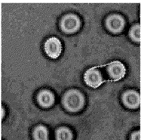
–2 q( 1q3+q2q4) = p x f( , ) = z x f( , )2Figure 3.1: The original image (top); the
attractor image computed with the gradient method (middle); estimate of magnitude of local orientation (bottom).
3.4 A
TTRACTING TOP
LANARS
TRUCTURE IN3D I
MAGES9
Computer Vision Laboratory, Linköping University
edges in directions separated by . The norm can then be calculated as
(3.9) What is important in order to get a good esti-mate, though, is that the filters together cover all directions.
In Figure 3.1 an image is filtered with the gra-dient method and the orientation method. Both methods uses four filters (line detecting and line/edge detecting respectively) applied in two scales. The gradient method is the same as in the example in Section 2.3 and according to (3.1). The orientation method is used according to (3.7) and (3.8).
3.4
A
TTRACTING TOP
LANARS
TRUCTURE IN3D I
MAGESAs described in [6] one can weight the line/edge filters mentioned above and estimate the orienta-tion tensor T, whose eigensystem describes the local variation of the signal (or the local energy distribution in the Fourier domain) and therefore also the orientation.
Calling T’s eigenvalues λ1, λ2 and λ3, where λ1≥ λ2≥ λ3, and the corresponding eigenvectors e1, e2 and e3, there are (in 3D) three characteris-tic cases:
• Plane case: λ1>>λ2 λ3 0
The signal varies mainly in one direction, e1, i.e the spatial neighbourhood describes a pla-nar structure, with e1 as normal vector (the plane is spanned by e2 and e3). The energy in the Fourier domain is mainly distributed along a line in the direction of e1.
• Line case:λ1 λ2>>λ3 0
The energy in the Fourier domain is distrib-uted on a plane spanned by e1 and e2. The spatial neighbourhood is (nearly) constant in the same direction and describes a linear structure along e3.
2. Or eight real filters.
3. Actually, any number (equal or greater than three) of filters can be used. The estimation will be more se-cure the larger the number and the smaller the radial bandwidth of the filters. This decrease of bandwidth will however increase the spatial size of the filters, making the orientation estimate less local.
• Isotropic case:λ1 λ2 λ3
The neighbourhood has no orientation, i.e it varies equally in all directions.
Using a certainty estimate as attractor
In 3D, a signal containing planar structure is a simple signal. Thus, an estimate of planar struc-ture is
, (3.10)
i.e how much the orientation tensor differs from the tensor corresponding to a simple signal in the direction of dominant orientation.
The spectrum theorem states that
(3.11) and since the norm can be cal-culated as
(3.12)
will be close to zero in the presence of planar structure, and computation of (3.12) in each point in the image creates an attractor image that will attract the contour to planar structures in the image.
will also be close to zero when all eigen-values are small. Consequently is very sen-sitive to noise on low-energy parts of the image, and therefore a division by λ1 is suitable. The attractor image can then be expressed as
(3.13) where , (3.14) π⁄3 z2 qk 2 k=1 3
∑
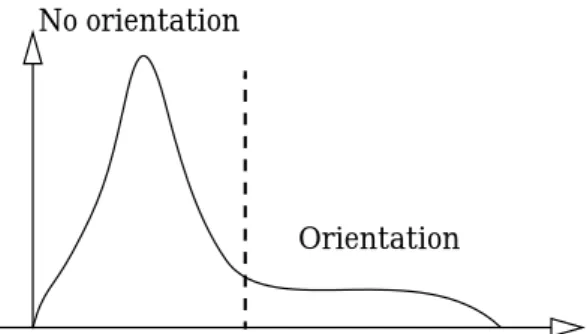
–q1q2+q1q3+q2q3 = 3×3 ≈ ≈ ≈ ≈ ≈ ≈ ∆( )T = T–T1 T1 λ1 e1e1 T ⋅ = T λ1 e1e1 T ⋅ λ2 e2e2 T ⋅ λ3 e3e3 T ⋅ + + = e2e2 T e3e3 T ⊥ ∆( )T ∆( )T T–T1 λ2 e2e2 T ⋅ λ3 e3e3 T ⋅ + = = λ2 2 λ3 2 + = ∆( )T Orientation Noisy background No orientationFigure 3.2: Histogram of an attractor
image. ∆( )T ∆( )T p∆(x f, ) = –∆λ(eigenv alues T x f( ( , ))) ∆λ( )λ λ2 2 λ3 2 + λ1 ---= ∆λ:ℜ3→ℜ
10
C
HAPTER3: T
HEA
TTRACTORI
MAGEActive Contours in Three Dimensions
If the attractor image is calculated according to (3.13), the “typical” histogram look like Figure 3.2. Pixels within isotropic neighbourhoods will have lower values than the “oriented” pixels, but pixels within isotropic neighbourhoods domi-nated by noise (e.g., noise added to a black back-ground) will have higher values (see Figure 3.2), i.e close to the oriented pixels.
Another certainty estimate
The interesting case of the cases mentioned above is the plane case, i.e., whenλ1>>λ2 λ3. Thus, the quota
(3.15) is a certainty estimate of planar structure, which varies between one and one third. As with the first certainty estimate when all the eigenvalues are small, the quota (3.15) will be quite random. It is therefore suitable to multiply the quota with λ1 to reduce the sensitivity to noise.
The attractor image used will consequently be expressed as
(3.16) where
, (3.17)
A typical histogram of the attractor image computed according to (3.16) will look like Figure 3.3. The oriented and isotropic areas seems not to be as well separated as with (3.13), but this method is not as sensitive to noise. The choice of method should therefore depend on how noisy the image is around the object one wishes to seg-ment.
3.5
C
REATING THEA
TTRACTORI
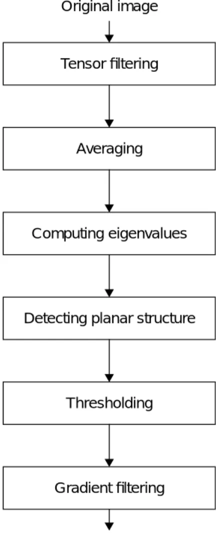
MAGEAs indicated above, several steps are required to create the attractor image and the resulting image force. The sequence of these steps is illus-trated in Figure 3.4 and described below (a 3D-image is assumed).
1. Tensor filtering
Filter the image with at least six edge/line-detectors and create the orientation tensor according to Section 3.4.
2. Averaging
The tensor field usually needs some averaging (low-pass-filtering) to reduce randomness of the orientation caused by noise. An ordinary or gaussian kernel is used.
3. Computing eigenvalues
Compute the eigenvalues of the tensor field and sort them in decreasing order.
4. Detecting planar structure
Compute the energy according to equation (3.16) or (3.13).
5. Thresholding
The parts of the original image without domi-nant local orientation, e.g black background, will (especially in the presence of noise) con-tribute to the calculated attractor, however with quite low values. It is, though, preferable to set all these points to zero. This will straighten out the contour where crossing such regions, since the contour will there only be under the influence of the internal forces (elasticity and rigidity).
The typical histogram (see Figure 3.3) is mainly divided into two ares; all uninterest-ing pixels (“isotropic case”) have low values and the pixels with planar structure have higher values. Setting all pixels in the “iso-tropic area” to zero and subtracting this value from the other pixels results in a more relia-ble attractor image.
≈ λ1 λ1+λ2+λ3 ---pc(x f, ) = c eigenv alues T x f( ( ( , ))) c( )λ λ1 2 λ1+λ2+λ3 ---= c :ℜ3→ℜ Orientation No orientation
Figure 3.3: Histogram of an attractor
image.
3.5 C
REATING THEA
TTRACTORI
MAGE11
Computer Vision Laboratory, Linköping University
If the second certainty estimate is used, then a (variable) threshold of slightly more thanλ1/3 will set all “isotropic pixels” to zero.
6. Gradient filtering
Computing the 3D-gradient of the attractor image will result in the image force used when iterating the contour. The image force is a function , i.e., every “pixel” in the 3D-image is a three-element vector.
Tensor filtering
Computing eigenvalues
Detecting planar structure
Gradient filtering Thresholding Original image
Image force Averaging
Figure 3.4: The process of calculating the
image force.
13
4
4
R
EPRESENTATION IN
T
HREE
D
IMENSIONS
This chapter treats the basic extension of the active contour model from two to three dimensions. Different representations of 3D con-tours are described, which also makes it necessary to revisit the methods of calculating the internal forces.
4.1
T
HE3D C
ONTOURA 3D contour is typically described by a function . The contour is placed on an image and is moved by iteration in the same way as in the 2D case.
The simplest way to create an active contour in 3D is by using repeated 2D contours. This method is often used since it is also quite intui-tive in many applications with image sequences. The major drawback is that it is impossible to vary the distance between the control points in the third dimension, so that exactly one point per pixel (in the third dimension) is required.
In some applications (e.g., [2] and [7]) one does not even care about elasticity and rigidity in the third dimension and calculates a number of inde-pendent contours on separate images. This, of course, can result in very unpleasant contours, e.g., if a piece of a line through the image sequence is missing in one or some images.
In this thesis, “true” 3D contours are dis-cussed, i.e., the control points can move in three directions and both the external and internal forces operate in 3D.
4.2
T
HEE
NERGY OF THEC
ONTOURIn 3D the image force is defined in the same way as in 2D, but the internal energy has to be calcu-lated in a slightly different way, which also leads to a modification of the Euler-Lagrange-equation (2.5).
To calculate the internal energy in 3D, some additional parameter functions are required, and the energy is now defined as (with )
Eint= (4.1)
where and determine the elasticity along the s- and r-axis respectively, and deter-mine the corresponding rigidities and deter-mines the resistance to twist.
The energy is minimized by finding the v that satisfies the Euler-Lagrange-equation
(4.2)
which, as in 2D, means that the internal forces shall balance the image force.
4.3
R
EPRESENTATIONA 2D contour is simply represented by a vector of control points where neighbouring control points are represented by neighbouring elements in the vector. (This is what causes the matrix A in (2.8) - (2.9) to be pentadiagonal.)
In 3D, the contour is most easily represented by a matrix of control points, a mesh. The mesh is not suitable in all cases; this will be discussed below. v : 0 1[ , ]×[ , ]0 1 →ℜ3 f :ℜ3→ℜ v = v s r( , ) αsvs' 2 αrvr' 2 βs + vss'' 2 βrvrr'' 2 βsrvsr'' 2 + + + ( )dsdr
∫
αs αr βs βr βsr p v f( , ) ∇ +αsvss''+αrvrr'' βsvssss 4 ( ) β rvrrrr 4 ( ) – βsrvssrr 4 ( ) – – = 014
C
HAPTER4: R
EPRESENTATION INT
HREED
IMENSIONSActive Contours in Three Dimensions Representing the contour with a mesh
The two different types of 2D contours (open and closed contours) can with the corresponding boundary conditions
(4.3) (4.4) be extended to a cylinder if one of (4.3) and (4.4) is met or a torus if both (4.3) and (4.4) are met. If none of the conditions are met, the contour is just an open surface.
Assuming an n×m-mesh, it is trivial to expand
the mesh to an n(n - a)×m(m - b)-mesh, where a
and b equal one if equation (4.3) and (4.4) respec-tively are satisfied (and zero otherwise).
Representing the contour with a polyhedron
To create a sphere-like contour one can use the following set of boundary conditions:
(4.5) (4.6) (4.7) However the control points will then be placed on the sphere in a quite irregular manner (with regard to their mutual distances), and there is no obvious way to modify (4.1) to fit this topology. Consequently the mesh-representation is not suitable for spherical contours - instead it is pref-erable to place the control points regularly on a sphere, i.e., to let the control points be the verti-ces of a regular polyhedron (in case of eight con-trol points, they should be placed like the corners of a cube). Unfortunately there is no regular
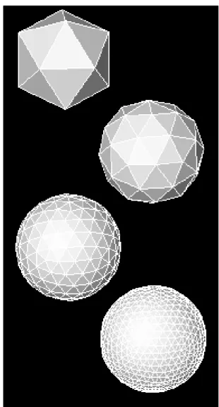
polyhedron with more than twenty vertices, as proved by Plato some time ago [4].
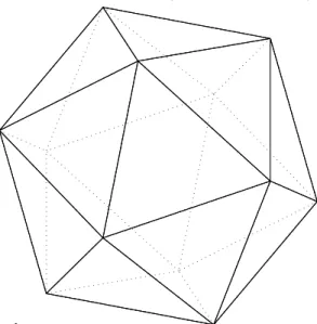
A solution is to create a quasi-regular polyhe-dron with equal distances between each vertex and its neighbours. Such polyhedra can be cre-ated recursively from an icosahedron, see Figure 4.1, using the following algorithm:
1. Place a new vertex at the midpoint of each edge.
2. Remove the old edges and create new edges
between all vertices with a mutual distance that equals half of the distance between the old vertices.
3. Project the new vertices on the circumsphere of the polyhedron.
The original twelve vertices have five neighbours while all new vertices will have six neighbours. The number of faces, edges and vertices (Fn, Enand Vn where n is the number of recur-sions) grow quite quickly. The original polyhe-dron P0 has got the characteristics
(F0E0V0) = (20 30 12), and the characteristics of polyhedron Pn is calculated recursively (directly from the algorithm) as
(4.8)
Expanding En as
En (4.9)
(and so on) makes it obvious that En can be writ-ten as a closed expression:
En (4.10) v s 0( , ) = v s 1( , ) s∀ v 0 r( , ) = v 1 r( , ) r∀ v s 0( , ) = v s 1( , ) s∀ v 0 r( , 1)= v 0 r( , 2)∀r1,r2 v 1 r( , 1)= v 1 r( , 2)∀r1,r2
Figure 4.1: The icosahedron, one of the five
Platonic polyhedra. Fn= 4 F⋅ n–1 En= 2En–1+3Fn–1 Vn=Vn–1+En–1 2 2E( n–2+3Fn–2)+3Fn–1 = 2 2 2E( ( n–3+3Fn–3)+3Fn–2)+3Fn–1 = 2nE0 3 2 n–1–k k=0 n–1
∑
Fk ⋅ ⋅ + = 2nE0 3 2 n–1 2–k∑
F0 4 k ⋅ ⋅ ⋅ ⋅ + = 2nE0 3 2 n–1 F0 2 k∑
⋅ ⋅ ⋅ + = 30 4⋅ n =4.4 T
HEI
NTERNALF
ORCESI
NDEPENDENT OFR
EPRESENTATION15
Computer Vision Laboratory, Linköping University
In a similar way Vn can be expanded and expressed as
Vn (4.11)
Fn is trivially rewritten, and so (4.8) equals
(4.12)
For example, P3 and P4 have 642 and 2562 ver-tices respectively, which could be suitable amounts in practical applications. The four first polyhedra (P0 through P3) are illustrated in Fig-ure 4.2.
4.4
T
HEI
NTERNALF
ORCESI
NDEPENDENT OFR
EPRESENTATIONElasticity can be regarded as a dragging force from each of the neighbouring control points, i.e., the elasticity force in a control point is simply the vector from the control point to the average of the neighbouring control points (see Figure 4.3). In 2D, this is the same as equation (2.6).
Figure 4.3: The elasticity force drags the
control point vj towards the average of the control points vj-1 and vj+1.
Rigidity can be regarded as the force from a control point to a point linearly “predicted” by the two “earlier” points, as shown in Figure 4.4, i.e., the vector from vj-2 to vj-1 is added to vj-1, and
vj is forced towards the resulting point. This means that the rigidity force in a point vj is . The “prediction” can be made in all directions and be generalized to higher dimensionality.
Figure 4.4: The rigidity force drags the
control point vj towards the position predicted by the control points vj-2 and vj-1. The control points vj+2 and vj+1 creates a similar force.
This view of rigidity is not the same as the physical property; it will not straighten lines by suppressing corners but by raising neighbouring points to the same level as the corner. By adding twice the elasticity to the rigidity it becomes the same.
This can more formally be expressed in the fol-lowing way:
Figure 4.2: The icosahedron and its first
three expansions. V0 Ek k=0 n–1
∑
+ = 12+30⋅∑
4k = 2+10 4⋅ n = Fn 20 4 n ⋅ = En 30 4 n ⋅ = Vn 2 10 4 n ⋅ + = vj-1 vj vj+1 2vj–1–vj–2–vj vj-2 vj-1 vj16
C
HAPTER4: R
EPRESENTATION INT
HREED
IMENSIONSActive Contours in Three Dimensions
Let , , be the set of
M points on a distance d steps from a control
point vj. By setting cj,d to the average of all points on the distance d from the point vj, i.e.,
(4.13) the elasticity and rigidity forces in the point vj can be expressed as
(4.14) (4.15) These equations are applicable on a contour in 2D as well as on a mesh (describing a surface, torus or cylinder) or a polyhedron. Their best use
is however on the polyhedron, where it is not obvious how to calculate the s- and r-derivatives. They also make it possible to choose whether to use 4-connectivity or 8-connectivity in the mesh.
The elasticity and rigidity parameters are then again only two - (for elasticity in all direc-tions) and (for rigidity in all directions) - and the sought-for balance of the contour forces is now expressed as
(4.16) where is the set of control points representing the contour v. If is a vector (4.16) equals (2.5), and if is a mesh with 4-connectivity (4.16)
equals (4.2) with , and .
Pj d, = {pj d m, , } m = 1, ,… M cj d, pj d m, , Pj d, ---m
∑
= Felast( )vj = cj 1, –vj Frigid( )vj = 4cj 1, –cj 2, –3vj α β α⋅Felast( )v +β⋅Frigid( )v +∇p v f( , ) = 0 v v v αs = αr βs = βr βsr = 017
5
5
R
OBUST
C
ONTROL
This chapters examines the problem of instability due to internal forces, which are too strong but which are still too weak to fulfil their purpose. The suggested solution limits the internal forces’ influence on the shape of the contour, instead letting them influ-ence the point distribution only. This also makes it possible to use the balloon-concept in a stable way.
5.1
T
HEP
ROBLEM OFS
ENSITIVEP
ARAMETERSThe purpose of the elasticity force is to keep the control points equidistant along the contour. However, if the distance between the control points is too large on an overly curved image con-tour, the elasticity force tends to drag the control points away from rather than along the image contour; see Figure 5.1.
This can be avoided by decreasing the values of the elasticity parameter function α(s), but a
too weak elasticity force (compared to the image force) makes the points gather in strong areas on the attractor image in a very non-equidistant manner. To find an α(s) (and a β(s)) that solves
the problem, it may be necessary to set its values individually in each point, but even then it is not certain that a solution exists.
5.2
O
UTLINE OFS
OLUTIONXu et al. suggest in [14] that the tangent of the contour should be approximated at each control point, and that a pressure force perpendicular to the tangent should be added. This force has in each control point the same magnitude as the part of the internal force that is perpendicular to the tangent, but the two forces shall point in opposite directions and consequently balance each other. As a result the internal forces may only move a control point along the direction of the tangent.
A simpler way to express the same thing is that the elasticity force should be projected on the tangent plane of the contour before influenc-ing the contour.
The problem is then reduced to approximating the tangent, or, in 3D, the tangent plane, in each point. Two methods are described below.
vj-1 vj vj+1 Felast vj-1 vj vj+1 Felast vj-2
Figure 5.1: An overly strong elasticity force, Felast, drags the control point vj away from the image contour (left), while a weak elasticity force cannot keep the points equidistant (right).
18
C
HAPTER5: R
OBUSTC
ONTROLActive Contours in Three Dimensions A comment on complexity of algorithms
Only computational complexity (complexity in time) is considered here, since the complexity in space (i.e., memory) is in any case very small compared to the space needed for the attractor image.
The computational complexity is approxi-mated by the number of floating point operations needed. Fixed point operations for program con-trol, etc., are regarded as taking zero time.
5.3
R
ECONSTRUCTING AC
ONTOURU
SINGB
ASISF
UNCTIONSIf the contour is represented by a mesh, we can regard the control points as a regular sampling of a signal. We can then reconstruct the signal as a linear combination of a set of basis functions with the values in the sampling points as coeffi-cients.
Assuming the signal is limited to a finite range/area/volume in the Fourier domain, a per-fect reconstruction is possible. For a signal to be band-limited, it must be unlimited in space, and therefore only closed contours (periodic signals) can be band-limited.
Requirements on basis functions
For a set of functions to be used as basis func-tions the following requirements have to be met:
• The functions should equal zero in all sam-pling points but the one corresponding to the basis function.
• The sum of all basis functions should equal one in all points (not just in the sampling points).
• The functions should belong to a Sobolev-space of the fourth order, i.e., all derivatives of up to the fourth order should be squared inte-grable. If not, the rigidity force does not neces-sarily converge.
Choice of basis functions
If the contour is closed in a dimension (i.e., equa-tion (4.3) or (4.4) in Secequa-tion 4.3 is satisfied), we can use a band-limited periodic function as the basis in that dimension. Its period should equal the length of the contour, and a suitable basis function (if the number of samples is odd) is
(5.1)
where n is the number of samples and the other basis functions in the set are the translations . The derivative function of the m:th order is then given by
(5.2) In case of an open contour it is not possible to use band-limited functions. Instead the open con-tour can be regarded as a small part of a much larger (closed) contour, whose sampled values all equal zero outside the limited part.
For example, (5.1) can be used as a basis func-tion, but with an n at least twice the number of samples (in order for two points to correlate less as the distance between them grows).
Reconstruction of the contour and its derivatives
The contour can be written as (5.3) with the derivatives
(5.4)
Assuming the contour to be represented by three -meshes , and the deriva-tives in a control point (s1, s2), sj∈{0, ... , nj- 1}, equal
(5.5)
The values of the functions can be calculated in advance (i.e outside the iteration-loop) and the values stored in vectors
(5.6) ϕn( )x 1 n --- 1 2 2kπx n --- cos k=1 n–1 ( )⁄2
∑
⋅ + = ϕn(x–k) ϕn m ( ) x ( ) 2 n --- 2kπ n --- m 2kπx n --- mπ 2 ---– cos k=1 n–1 ( )⁄2∑
⋅ = v :ℜ2→ℜ3 v s( 1,s2) x1(s1,s2) x2(s1,s2) x3(s1,s2) T = sk m m ∂ ∂ v sk m m ∂ ∂ x1 sk m m ∂ ∂ x2 sk m m ∂ ∂ x3 T = n1×n2 x1 x2 x3 s1 m m ∂ ∂ xj xj(k s, 2) ϕn1 m ( ) s1–k ( ) ⋅ k=0 n1–1∑
= s2 m m ∂ ∂ xj xj(s1,k) ϕn2 m ( ) s2–k ( ) ⋅ k=0 n2–1∑
= ϕnj m ( ) x–k ( ) ϕn m ( ) s ( ) ϕn m ( ) s ( ) ϕn m ( ) s–(n–1) ( ) =5.3 R
ECONSTRUCTING AC
ONTOURU
SINGB
ASISF
UNCTIONS19
Computer Vision Laboratory, Linköping University
Using (5.6) and the matrix given by
(5.7)
(and the corresponding ) the derivatives can be expressed as
(5.8)
Since the values of the basis functions can be calculated in any point, it is possible to interpo-late the contour and its derivatives in any point (s1, s2). If neither of s1 or s2 are integer values, the contour v(m) has first to be interpolated in all the points (s1, 0) ... (s1, n2- 1) (using the second
equa-tion in (5.8)). Then v(m)(s1,s2) can be reconstructed using the first equation in Figure 5.8.
The tangent plane
The tangent plane of the contour is given by its normal vector
(5.9) which by insertion of (5.8) can be expressed as
(5.10)
Computational complexity
Computing (5.8) requires 6(n1+ n2- 1) floating
point operations. Another 9 operations are needed to calculate the normal vector µ, so a total of 6(n1+ n2) + 3 operations are needed to
cal-culateµ in one point, i.e in O(n1+ n2) time. xs1( )s2 x1(0 s, 2) … x1(n1–1,s2) x2(0 s, 2) … x2(n1–1,s2) x3(0 s, 2) … x3(n1–1,s2) = xs2( )s1 s1 m m ∂ ∂ v s 1,s2 ( ) xs1( )s2 ϕn1 m ( ) s1 ( ) = s2 m m ∂ ∂ v s 1,s2 ( ) xs2( )s1 ϕn2 m ( ) s2 ( ) = µ s1 ∂ ∂v s2 ∂ ∂v × = µ(s1,s2) xs1( )s2 ϕn1 m ( ) s1 ( ) xs2( )s1 ϕn2 m ( ) s2 ( ) × = 15 20 25 30 35 40 45 50 55 15 20 25 30 35 40 45 15 20 25 30 35 40 45 50 55 15 20 25 30 35 40 45 15 20 25 30 35 40 45 50 55 15 20 25 30 35 40 45 15 20 25 30 35 40 45 50 55 15 20 25 30 35 40 45
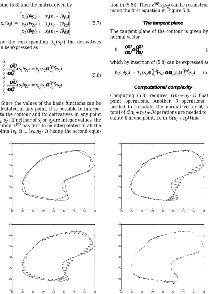
Figure 5.2: The contour represented by 11 control points and its reconstruction (top left); the
rigidity force (top right); the elasticity force (bottom left); the elasticity force projected on the tangent in each point (bottom right).
20
C
HAPTER5: R
OBUSTC
ONTROLActive Contours in Three Dimensions Global internal forces
Equation (5.8) can be also used to calculate the elasticity and rigidity forces. Compared to using the earlier methods (e.g., equations (4.14) - (4.15) in Section 4.4) this will increase computation complexity by a factor proportional to n1+ n2. As a positive effect the internal forces will behave globally, i.e., if when a control point is moved, the force on all other points will be immediately effected, instead of several iterations later.
An example
In Figure 5.2, a 2D-contour with 11 control points is interpolated in 55 points using the basis function (5.1). Its second and fourth derivatives, i.e the elasticity and the rigidity force respec-tively, are interpolated as well.
5.4
A
PPROXIMATING THET
ANGENTP
LANE WITHS
PHERESOn a generalized representation of the contour, e.g., the polyhedron-representation described in Chapter 4, the method described above cannot be used (unless a way of expressing basis functions for a general polyhedron can be found). Instead, an approximating method will be used.
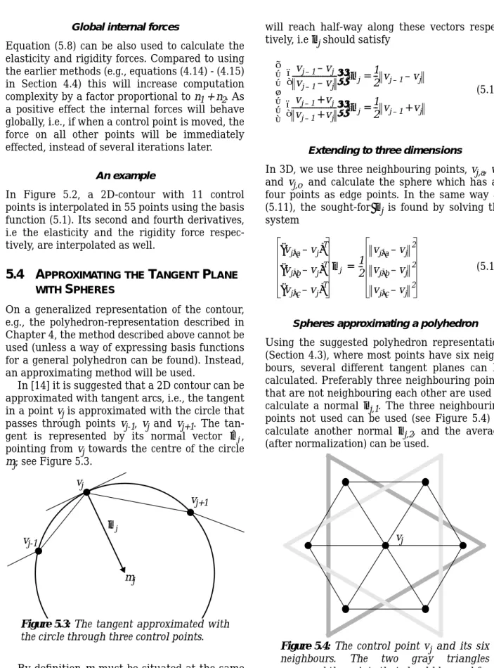
In [14] it is suggested that a 2D contour can be approximated with tangent arcs, i.e., the tangent in a point vj is approximated with the circle that passes through points vj-1, vj and vj+1. The tan-gent is represented by its normal vector , pointing from vj towards the centre of the circle
mj; see Figure 5.3.
Figure 5.3: The tangent approximated with
the circle through three control points.
By definition mj must be situated at the same distance from vj-1, vj and vj+1, which implies that µj projected on vj-1- vj and vj+1- vj(see Figure 5.3)
will reach half-way along these vectors respec-tively, i.eµj should satisfy
(5.11)
Extending to three dimensions
In 3D, we use three neighbouring points, vj,a, vj,b and vj,c, and calculate the sphere which has all four points as edge points. In the same way as (5.11), the sought-for µj is found by solving the system
(5.12)
Spheres approximating a polyhedron
Using the suggested polyhedron representation (Section 4.3), where most points have six neigh-bours, several different tangent planes can be calculated. Preferably three neighbouring points that are not neighbouring each other are used to calculate a normal µj,1. The three neighbouring points not used can be used (see Figure 5.4) to calculate another normal µj,2, and the average (after normalization) can be used.
Figure 5.4: The control point vj and its six neighbours. The two gray triangles surround the points that should be used for calculatingµj,1 andµj,2 respectively.
Some care is needed doing the averaging. If the two normal vectors are related like µˆj vj-1 vj vj+1 µj mj vj–1–vj vj–1–vj --- µ j ⋅ 1 2 --- vj–1–vj = vj–1+vj vj–1+vj --- µ j ⋅ 1 2 --- vj–1+vj = vj a, –vj ( )T vj b, –vj ( )T vj c, –vj ( )T µj 1 2 ---vj a, –vj 2 vj b, –vj 2 vj c, –vj 2 = vj
5.5 C
ONTROLLING THEC
ONTOUR21
Computer Vision Laboratory, Linköping University
the average will point in a random direction. This is avoided by definingµj as
(5.13) where
(5.14) On the twelve points on the polyhedron which have only five neighbours,µj has to be calculated differently. To get a symmetrical distribution of spheres, five spheres are needed, each sphere using the control point in which the tangent should be calculated, one neighbouring control point vk and the two points neighbouring vj but not vk. The resulting normal is then calculated by generalizing (5.13):
(5.15)
where N is the number of spheres (i.e 5).
Alternatively, only one sphere is calulated, hoping that three neighbouring points are enough for a good approximation.
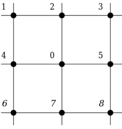
Spheres approximating a mesh
Using 8-connectivity, the tangent plane of a mesh can be approximated with four spheres. Number-ing the neighbours accordNumber-ing to Figure 5.5 we calculate the four spheres using the following sets of points: {0, 4, 3, 8}, {0, 2, 6, 8}, {0, 5, 1, 6}, {0, 7, 1, 3}. The resulting µj,1,..., µj,4 are used according to (5.15) to calculateµj. The alternative mentioned above, i.e., to calculate only one of theses spheres, is still valid.
Figure 5.5: A numbering of control points.
Computational complexity
Using Cramer’s rule [10] stating1
(5.16) to invert the matrix in (5.12), the inversion can be done making 27 floating point operations. (Since we do not care about the length of the vec-tor µj, it is not necessary to calculate .) Creating the vector on the right hand in (5.12) needs 24 operations, and multiplying it with A-1 needs another 15 operations. This adds up to 66 operations to solve the system (5.12) and calcu-late one sphere.
Equation (5.15) needs 11⋅(N - 1) operations plus another 9N operations for normalizing the vec-tors. Summing up, there is need for 86N - 11 oper-ations to calculate the normal vector.
Comparing this with the method suggested in Section 5.3 (using basis functions), sphere-fitting is faster except for on a very small mesh.
5.5
C
ONTROLLING THEC
ONTOURProjecting the elasticity on the tangent plane before it influences the shape of the contour makes the contour more stable and less sensitive to the choice of parameters. Using a constantα of
0.5, which makes the points move to the
(cur-rently) ideal position in each iteration, should no longer change the shape of the contour signifi-cantly.
By projecting the rigidity on the tangent plane as well, the contour can hold on to shapes in the images that have a high degree of curvature (without changing the parameter β in selected points). The contour has of course lost most of its rigidity but will now keep approximately the same size and shape (except for by influence from the attractor image).
The contour can now be controlled by adding another force, a user-controlled inflation force, to give the contour the preferred size. This makes it possible to “guide” the contour to the interesting part of the image by manipulating only one (glo-bal) parameter. This is the same idea as the bal-loon model described in [1].
For example, when trying to find the inside of a ventricle, a small spherical contour (polyhe-dron) could be placed in the middle of the ventri-cle and inflated to approximately the correct size. Then, the contour can be turned active again, by 1. B = adj(A) denotes the matrix of which the element bij
equals the cofactor of the element aji in A. µˆj 1, ≈–µˆj 2, µj = µˆj 1, +sign(µj 1, ⋅µˆj 2, )µˆj 2, sign x( ) 1 if x≥0 1 – if x<0 = µj µˆj 1, sign(µˆj 1, ⋅µˆj k, )µˆj k, k=2 N
∑
+ = 0 1 2 3 4 5 6 7 8 A–1 adj A( ) det A( ) ---= det A( )22
C
HAPTER5: R
OBUSTC
ONTROLActive Contours in Three Dimensions
no longer projecting the rigidity and resetting the inflation force.
The force influencing a control point vj can now be expressed as
= (5.17)
whereγ is the user-controlled parameter regulat-ing the inflation force andε is the parameter tell-ing the contour to be active or inactive, i.e.,
(5.18)
When calculating the inflation force it is important that all normal vectorsµj are pointing in the “same” direction. That is, on a spherical contour, all normal vectors should point towards the outside of the contour (or inside, but they should all be alike). If the normal vectors are cal-culated using spheres, this is only guaranteed if the contour is convex. The problem is not trivial, but since it depends on the implementation it is not treated here. A solution is described in Appendix B, “Implementation in 3D”. F v( )j α(Fe last( )vj –(Fe last( )vj ⋅µˆj)µˆj) β(Fr igid( )vj –ε(Fr igid( )vj ⋅µˆj)µˆj) γ µˆj–∇p v( j, f) + + ε 1 if γ >0 0 otherwise =
23
6
6
E
XPERIMENTS
This chapter describes the experiments performed to test the meth-ods suggested in earlier chapters. Two experiments were per-formed; one with ideal, mathematically defined image volumes and one with “real” medical image volumes.
6.1
T
HEA
CTIVEC
ONTOURM
ODELThe active contour model was implemented as C++ classes and AVS modules, as described in Appendix B.3, “The Active Contour Model”.
The internal forces in the control points were computed as defined in Section 4.4, i.e., as
(6.1) (6.2) where is the average of all control points on the distance i from the control point vj. The iterations were performed according to
(6.3) where the force F(vj) in each control point is
com-puted as
= (6.4)
α,β andγ are the parameters regulating the elas-ticity, the rigidity and the inflation force respec-tively, and are the parameters telling the internal forces to be active or inactive (i.e., if they should be projected on the contour’s tangent plane or not). The function clip limits the image force vector to the lengthδ.
Note that the iteration-method in Equation (6.3) is not the same as Equation (2.9) (Euler’s method). Instead, each control point is moved according to the sum of all forces. This method converges somewhat slower but is extremely easy to implement in O(n)-time.
The normal vectors were approximated using the sphere-fitting method described in Section 5.4.
6.2
F
ITTINGC
ONTOURS TOS
YNTHETICS
HAPESTwo test volumes were constructed, one for test-ing each representation (mesh and polyhedron; see Chapter 4). The purpose to measure the per-formance of the contours, since the intended shapes are well defined. The volumes used were:
• The “half-sphere” volume for testing the poly-hedron representation: A pixel volume where the pixels on a half-sphere and the pixels in the circle that cuts the sphere have the value one. The rest of the pixels are set to zero.
In addition, an area on the half-sphere has its values multiplied with three, thus intended to attract the contour more strongly and disturb the point distribution. The vol-ume is illustrated in Figure 6.1.
vj ℜ 3 ∈ Felast( )vj = cj 1, –vj Frigid( )vj = 4cj 1, –cj 2, –3vj cj i, ℜ 3 ∈ vk+1 = vk+F v( )k F v( )j α(Fe last( )vj –ε1(Fe last( )vj ⋅µˆj)µˆj) β(Fr igid( )vj –ε2(Fr igid( )vj ⋅µˆj)µˆj) γ µˆj clip(δ,∇p v( j, f)) + + + εi∈{ , }0 1 60×40×60
Figure 6.1: The ‘half-sphere’. The pixels