Deformation of human soft tissues
Experimental and numerical aspects
Licentiate ThesisSara Kallin
Jönköping University School of Engineering
Licentiate thesis in Machine Design Deformation of human soft tissues – Experimental and numerical aspects Dissertation Series No. 049
© 2019 Sara Kallin Published by
School of Engineering, Jönköping University P.O. Box 1026 SE-551 11 Jönköping Tel. +46 36 10 10 00 www.ju.se Printed by BrandFactory AB 2019 ISBN 978-91-87289-52-1
Acknowledgements
I would like to express my sincere gratitude to all who have supported me and made this work possible.
To my supervisors, Professor Peter Hansbo, Docent Kent Salomonsson and Professor Maria Faresjö for all their support and fruitful discussions during this work.
To Dr Asim Rashid for his engagement and collaboration in study I.
To all members of the PEOPLE project at Hotswap Norden AB, Ottobock Scandinavia AB and Ossur Nordic HF for their collaboration and support. I would like to express my appreciation to persons involved during tests of the questionnaire, the clinical assessment protocol and the development of equipment.
I gratefully thank the volunteering participant in study II, and Hans Eklund, Aleris Röntgen, Jönköping together with Anna Engdahl, Wetterhälsan, Jönköping, for collaboration in data collection.
For their financial support, the Jönköping Regional Research Programme, Sweden, the project PEOPLE, the School of Engineering and School of Health and Welfare at Jönköping University are greatly acknowledged.
To colleagues and friends at the School of Engineering, School of Health and Welfare and the community of Prosthetics & Orthotics for your support and encouragement, and for making my work more joyful.
Finally, I would like to thank my friends and family, especially my husband Jonas and daughters Sofia and Kristina, for your patience, support and love. To my father who always encourages me, Thank you.
Sara Kallin
Jönköping, Sweden July 2019
Abstract
Understanding human soft tissue deformation is important for preventing and decreasing the tissue damage due to mechanical load by external products. Experimental data for material properties of living human tissue are limited. Moreover, tissue tolerance to loads seems depend on the individual-specific conditions including health. Predictions of mechanical behaviour with finite element (FE) models exist, however FE simulations of human soft tissue apply simplified material representation of which impacts on outcomes are yet unclear. Strategies to investigate human tissue load response need to be improved for better understanding of tissue deformation.
This thesis aims to investigate aspects of deformation in human soft tissue of the leg when exposed to external loading. The focus is on soft tissue representation in FE simulation models and individual-specific live tissue deformation under established health conditions.
To investigate the influence of tissue material representation in FE simulation a strategy with a 2D generic multilayer model of the lower leg was introduced. Two material sets were applied, each representing skin, fat, vessels and bones separately while fascia and muscle tissues had either separate or combined material properties. External loads were applied by three different shapes of prosthetic sockets. The relative change between the two used material sets were considerable regarding the distribution and magnitudes of tissue’s stresses and strains as well as the contact pressures. Thus, the FE model was sensitive to how muscle and fascia were modelled. An experimental strategy for obtaining deformation in the leg tissues of a person with specified health condition was then developed and demonstrated in a case study. A tissue-indentation instrument (TIM) was designed so that the induced mechanical deformation could be captured by magnetic resonance imaging (MRI). A questionnaire and a clinical assessment protocol addressed health conditions related to pressure injury development. The investigated deformations were the displacement and stretch ratio λ per layer, the volume change by volume ratio J on cross-section slice and by the deformation gradient F and Jacobian determinant JFEM in a defined element within a specific muscle tissue region. Individual-specific results for one healthy male subject demonstrated that the layers of skin, fat, muscles and deep vessels were
IV
compressed and underwent large strains, while the connective tissues behaved incompressible and with small strains.
The combined results suggest that the deformation of the human lower leg soft tissue should be investigated by tissue types and layers, and represented by separate material behaviour instead of combined types and layers.
This work is relevant to the increase of the human tissue material property reference data set with subjects of diverse health conditions, and to verification and validation of related simulation models.
Key words: Human soft tissue, Deformation, Material property, Simulation, Finite element, Biomechanics, Pressure injury, Multidisciplinary
Nomenclature
aetiology the cause or origin of a disease anterior in front
anoxia lack of oxygen in body tissue connective tissue tissue which forms the
main part of bones and cartilage, ligaments and tendons, in which a large proportion of fibrous material surrounds the tissue cells
distal further away from the centre of the
body (is opposite to proximal)
epidermium outer nonvascular,
non-sensitive cell layer of skin
ex vivo experimentation or measurements
which takes place outside an organism, done in or on tissue from an organism in an external environment
fascia band or sheet of connective tissue,
primarily collagen, that attaches, encapsulates, stabilize and separate muscles and other internal organs
gluteal, gluteus muscles muscles in the
buttocks
hematoma collection of blood outside
blood vessels, e.g. in muscle tissues, mass
of blood under the skin
hypoxia inadequate supply of oxygen to
tissue or an organ
immobilize hinder movements, stop from
moving
immunological disease disease related to
the immune system
inferior lower down than another part inserts insoles (in current context) in vitro experiment which takes place in
the laboratory
in vivo in living tissue
ischemia deficient blood supply to part of
the body
lateral further away from the midline of
the body
limb extremity, leg or arm
liner a removable protective limb cover
item/layer worn between the skin and
inner surface of the prosthesis/orthosis (current context)
lymphatic referring to lymph
medial nearer to the central midline of the
body or to the centre of an organ
metabolism chemical transformations
within living cells for sustaining life, e.g. processing food/fuel to energy or to building blocks for proteins, breaking down organic matter
morphology study of the structure and
shape of living organisms, objects
necrosis death of a part of the body such
as a bone, tissue or an organ
occlusion blockage
orthosis, orthotic device externally
applied device used to modify the structural and functional characteristics of the neuro-muscular and skeletal systems oxygenation becoming filled with oxygen pathology study of diseases and the
changes in structure and function which diseases causes in the body
pathologies diseases, malfunctions,
abnormalities
periosteum dense layer of connective
tissue around a bone
peripheral arterial disease (PAD)
arterial vessel disease in peripheral body parts, such as feet and leg, and peripheral vessels, such as capillaries
physiology, human study of the human
body and its normal functions
posterior at the back
prominence part of the body which stands
out, e.g. bone knuckle.
prosthesis, prosthetic device externally
applied device used to replace wholly, or in part, an absent or deficient limb segment
prosthetic socket the individual specific
structural component encapsulating the residual limb/stump for axial and transverse stabilization of forces
proximal near the midline or the central
VI reactive hyperaemia congestion
(excessive fluid) of blood vessels after an occlusion has been removed
reperfusion return of blood supply after a
period of ischemia or hypoxia
residual limb the portion of a limb
remaining after an amputation
spinal referring to the spine, the
backbones, a series of bones linked together to form a flexible column
subcutaneous under the skin
subcutis, hypodermis subcutaneous fat superior higher up than another part trans-tibial through the tibia, shinbone,
crus
type 1 diabetes (T1D) the pancreas does
not produce insulin
type 2 diabetes (T2D) insulin resistance,
the body can’t use insulin properly (most common form of diabetes)
ulcer (open) sore in the skin
vascular disease disease affecting the
Symbols
σ sigma, mechanical stress
𝜀𝜀 epsilon, strain, engineering strain 𝜆𝜆 lambda, stretch ratio
𝐸𝐸 Green StVenant strain Young’s modulus of elasticity
L length, at deformed, current condition
L0 length, at undeformed, reference condition ∆ delta, denotes the difference on a variable 𝑒𝑒 Almansi finite strain
𝑇𝑇𝑇𝑇𝐸𝐸 Total potential energy 𝑈𝑈 Strain energy
𝑊𝑊 External work
F force
u displacement
𝜇𝜇 mu, shear modulus
µs coefficient of friction skin/indenter ∇ nabla, gradient
I matrix of unit entity, identity matrix 𝜈𝜈 nu, Poisson’s ratio
F deformation gradient, matrix
dX, dx a line element in undeformed and deformed state respectively 𝑪𝑪 = 𝑭𝑭𝑻𝑻𝑭𝑭 the right Cauchy-Green deformation tensor
b=FFT the left Cauchy-Green deformation tensor A a squared matrix named A
detA determinant of A
det 𝑭𝑭 determinant of the deformation gradient F
J Jacobian determinant
J Jacobian matrix
V0 volume, at undeformed, reference condition
VIII
Abbreviations
ABPI Ankle Brachial Pressure Index ABS Acrylonitrile Butadiene Styrene AMP Absolute Maximum Principal Strain BMI Body Mass Index
CAE Computer Aided Engineering CPO Certified Prosthetist-Orthotist CT Computed Tomography DIC Digital Image Correlation
DICOM Digital Imaging and Communications in Medicine DRV Damage Risk Volume
DTI Deep Tissue Injury
EPUAP European Pressure Ulcer Advisory Panel
FE Finite Element
FEA Finite Element Analysis FEM Finite Element Method FOV Field of View
kPa kilo Pascal
LVDT Linear Variable Differential Transformer MRI, MR Magnetic Resonance Imaging
NPUAP National Pressure Ulcer Advisory Panel PETG Glycol-modified Polyethylene Terephthalate PI Pressure Injury
PU Pressure Ulcer
RQ Research Question
Contents
1. Introduction ... 1
1.1. Problem statement... 1
1.2. Purpose and aim ... 2
1.3. Outline ... 3
2. Background ... 5
2.1. Human leg tissues ... 5
2.2. Soft tissue damage ... 8
2.2.1. Definition Pressure Injuries ... 8
2.2.2. Suggested mechanisms and factors ... 9
2.2.3. Prevalence of soft tissue damage related to PI ... 12
2.2.4. Evaluation of soft tissue status and PI ... 12
2.3. Deformation ... 13
2.4. Material models and parameters for large deformation ... 16
2.5. Experimental investigation of deformation ... 22
2.6. Computer simulations of soft tissue by Finite Element Method ... 24
2.6.1. Finite element method – a brief introduction ... 24
2.6.2. FEM in tissue biomechanics... 26
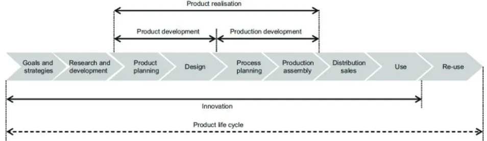
2.7. Position in the Industrial Product Realisation context ... 29
2.8. Rationale ... 31
3. Research approach ... 33
3.1. Scope and delimitations ... 33
3.2. Research perspective and strategy ... 35
3.3. Study I ... 36
3.3.1. Research design ... 36
3.3.2. The Finite Element Model ... 36
X
3.3.4. Boundary conditions ... 42
3.3.5. Procedures for analyses ... 43
3.4. Study II ... 44
3.4.1. Research design ... 44
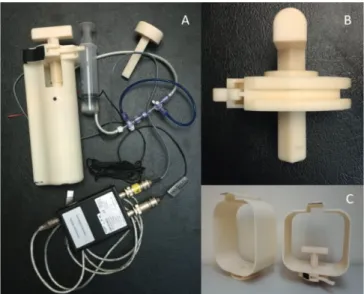
3.4.2. Equipment for deformation by indentation in MR ... 46
3.4.3. Clinical assessment ... 49
3.4.4. Questionnaire ... 50
3.4.5. Human subject ... 52
3.4.6. Data collection procedure ... 52
3.4.7. Data processing ... 54
3.5. Ethical considerations ... 59
4. Results ... 61
4.1. Study I ... 61
4.1.1. Comparisons of stresses and strains ... 61
4.1.2. Comparisons of contact pressures ... 66
4.2. Study II ... 68
4.2.1. Subject specific health conditions ... 68
4.2.2. Deformation measures from image analyses ... 70
4.2.3. Force-displacement by TIM ... 75
4.3. Geometry model from MR data in Study II ... 76
5. Discussion ... 77
5.1. Influence of differentiated tissue representation in FEA ... 77
5.1.1. Influence on stresses, strains and contact pressures ... 77
5.1.2. Discussion of the simulation model ... 79
5.2. Process for measuring individual-specific soft tissue deformation in separate tissue layers in vivo under established health conditions ... 82
5.2.1. Data collection techniques ... 83
5.3. Individual-specific soft tissue deformation measured in separate
tissue layers in vivo under established health conditions ... 90
5.3.1. Deformations ... 90
5.3.2. Health measures and clinical findings ... 92
5.4. Contribution ... 93
5.5. Implications ... 95
5.5.1. Tissue configurations in FE simulations ... 95
5.5.2. Individual specific tissue deformation in vivo ... 95
5.5.3. Product realization process ... 96
6. Concluding remarks ... 99 7. Future work ... 101 Sammanfattning ... 103 References ... 105 List of Figures ... 120 Appendices ... 123
I. Material parameters from indentation studies on human leg ... 125
II. Study II Clinical assessment protocol ... 130
III. Study II Questionnaire ... 137
IV. Study II Data collection sequence... 145
1. Introduction
1.1. Problem statement
In my profession as orthotist-prosthetist I meet individuals with diseases or physical disabilities who need external biomechanical supportive devices to facilitate their daily living activities. These external supportive devices, such as prostheses, orthoses, seating devices etc expose soft tissues to external loads and many users experience soft tissue problems. Different skin wounds and soft tissue problems may occur due to the interaction between the body tissues and the external supporting surfaces, manifesting as, for example, numbness, redness in skin, blisters, open wounds and sometimes deep tissue death (necrosis) [1]. Load-related wounds such as bedsores and pressure ulcers are also common in healthcare [2]. Problems in the loaded soft tissues may impact the person’s participation in activities. Severe ulcers may lead to amputation or even death. Tolerance of soft tissues to externally applied load is individual and varies with health status, age, morphology, skin conditions and mechanical properties of tissues [3]. It is therefore important to consider the individual’s soft tissue status and tolerance to load when managing the loading situation. The parameters for determining the soft tissue status in a clinical setting are often related to assessing the pathological condition by morphology (size, shape and structure), or aetiology (the cause, set of causes) of the conditions [3-8].
Moreover, the mechanisms of soft tissue behaviour and risk for damage when exposed to external loads are not yet fully understood. Several studies investigating specific biomechanical material properties in vivo have been performed over the years, but further investigations are still needed [9-12]. The multilayer configuration, diverse tissue structures and time dependence are challenging aspects of human soft tissues [9, 10, 13]. So far there is no established standard methodology for obtaining properties of individual-specific soft tissues [10, 14]. Additionally, little reference data for soft tissue materials from living humans are available.
Despite this, various mechanical material properties and material models have been used to represent the biomechanical behaviour of human tissues [9, 10, 13, 15]. The finite element method (FEM) is increasingly applied in
2
biomechanics to generate material properties, and for analyses of internal conditions of tissues exposed to loads. For these simulations diverse assumptions have been applied depending on the models used, available material properties, geometries and loading conditions. Examples of simplifying assumptions in models of human leg tissues are small strains, incompressibility and that specific tissue types and geometries have been merged together or neglected in the simulation models. For interpretation it is important to know how these simplifications influence the simulation results, but this is so far unclear. Using overly simplified simulations the error could be considerable [14]. There is a need to further explore effects of simplifications in simulation by FEM.
Hence, we need improved understanding of the deformation behaviour of soft tissues when exposed to load, as a compound and as separate tissue types and layers. In order to use simulation models for biomechanical analyses to decrease tissue damage and discomfort, we need further understanding of the influence of tissue representation in FE models for interpretation of simulation results. We need also to address the individual-specific conditions related to tissue behaviour including health related aspects. Thus, techniques to obtain such information on individual-specific level need to be further developed.
1.2. Purpose and aim
Thus, the overall purpose of this research is to improve the understanding of human soft tissue response when the body is interacting with external supports, such as improving methods for determining soft tissue behaviour, and representation in simulation models with FEM.
The specific aim is to investigate aspects of deformation in human soft tissue of the leg when exposed to external loading.
To achieve this aim, different aspects of this multidisciplinary problem are addressed in the context of mechanical conditions and health conditions related to tissue load tolerance. Analyses and measures of individual specific soft tissue behaviour, which include risk factors for pressure ulcers and health conditions, is part of this. The aim is wide, and further delimitations are
required. These will be addressed after the background chapter by the scope, research questions and delimitations in chapter 3.1.
1.3. Outline
A multidisciplinary approach was used, combining engineering, biomechanical and medical perspectives. Some preunderstanding from the engineering field is assumed. However, some concepts in one discipline require explanations for readers from another discipline and vice versa. This is a difficult balance, and the level of theoretical depth therefore varies in the thesis. A nomenclature is also provided to assist the reader. The outline of the thesis is as follows:
Chapter 1 describes the problem and aim of the research. The background, Chapter 2, describes human soft tissue and tissue damage due to load, some aspects of deformation, and introduces to varying extent related aspects, definitions and concepts that are used in the subsequent chapters. Experimental and numerical methods are reviewed as a basis for the research approach. Relations of this work to the industrial product realisation process are also presented here. In Chapter 3 the research questions, the chosen research approach and developed instruments are described. The initial simulation study provided insights to the subsequent experimental study, and these two studies addressed different aspects of deformation. Chapter 4 presents the results per study. In Chapter 5, the findings and methods are discussed in relation to the research questions, leading to the conclusions in Chapter 6. Future work is suggested in Chapter 7. Appendices are provided containing protocols and additional data.
2. Background
2.1. Human leg tissues
This research considers deformation in human soft tissues of the musculoskeletal system, the lower leg in particular. Therefore, a short description of the tissues of the lower leg based on Tortora [16] is introduced to the readers not familiar to human anatomy.
The lower leg is the structures between the knee and ankle and consists of many different tissues. Each tissue type is structured for its function and consists of different types of cells, often in layers.
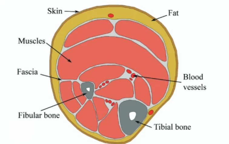
The skeleton of the lower leg includes the longitudinal bones tibia and fibula. The bone consists of cortical bone and bone marrow, while the joint surfaces of bones are covered by articular cartilage, a fibrous connective tissue with high water content. The bones are attached to each other with ligaments and membranes, made of connective tissues. The soft tissues of the lower leg are here defined as follows: the skin, subcutaneous fat, crural fascia, deep fascia inter-muscular dividers (septum) of connective tissue, intra-muscular fat, muscles, tendons, ligaments, blood vessels, nerves, and lymphatic vessels. They are organized in relation to each other in various ways, depending on the site and individual morphology. The transverse cross section at the height of upper third part on the lower leg is illustrated in Figure 1, based on Netter [17]. This cross section, at approximately the same level of leg height, is in focus for the research presented here.
6
Figure 1 Tissues at the mid-height of a human transtibial transverse cross section, the front of the leg, anterior, is up. (author)
The layers of tissues surrounding and connecting organs, as protecting bags, dividing walls and bands, are the fascia, epimysium, ligaments and tendons made of connective tissues. Fascia is like a sheet or broader band of fibrous connective tissue. A layer of fascia under the subcutaneous fat, the crural fascia (cruris Latin; from the leg), covers the internal soft tissues of the leg, with vessels and nerves penetrating it. Deep fascia is dense and irregular, dividing the muscles into groups with similar functions and allow them to move relative to each other. The fascia also provides channels for vessels and nerves. Tendons are fibrous bundles of connective tissues. The muscles and tendons move and stabilize the skeletal structures, and thus facilitate possibilities for physical activities.
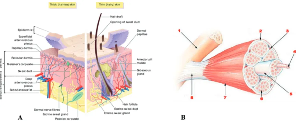
Skin and muscle tissue structures are illustrated in more detail in Figure 2. The human skin is a structure of interconnected layers, epidermis, dermis and subcutis/hypodermis (Figure 2 A). The underlying layer (named subcutis, hypodermis or subcutaneous fat) consists mainly of fat cells and connective tissues. Fibrous bands anchor this layer to the underlying crural fascia, while collagen and elastin fibres connect it to dermis. Blood vessels and nerves pass through this layer to dermis.
Figure 2 Skin and muscle tissue layers. A: Skin layers of human skin. B:Muscle tissue structure 1. Bone 2. Perimysium 3. Blood vessel 4. Muscle fiber 5. Fascicle 6.
Endomysium 7. Epimysium 8. Tendon. (Wikimedia Commons)
There are many muscles between the knee and ankle (examples in Figure 1). Each muscle consists of bundles of muscle fibres in groups, endomysium, divided by fascicles, Figure 2 B. The muscle outer layer, the perimysium, is encapsulated by another thinner layer of connective tissue, epimysium. These two layers can expand when the muscle contracts and shrink when the muscle relaxes or becomes thinner for other reasons. The epimysium will also contribute to sliding between neighbouring tissues.
Larger vessels for blood and lymphatic transportation are flexible tubes with walls of tissue layers of mainly connective tissue and muscle fibres. The nerves are bundles of hundreds to thousands of nerve cells, axons, within a thin protecting cover.
The interaction of human body soft tissue and external supports involves structures and mechanisms on different levels [1, 18]. A multilevel model adapted from Shoham and Gefen [18] and here applied to the musculoskeletal system of the human leg is suggested in Figure 3. ‘Macro level’ relates to the segment and site of the body where the external load is applied. ‘Meso level’ relates to the tissues and organs, e.g. skin, muscles, blood vessels, and the compound of tissue layers at a certain site. ‘Micro level’ relates to the cellular level, with the cell structure for each tissue type, and cellular functions, e.g. metabolism, transmission of substances through the cell membrane, signal substances for body system communication etc. When the body tissues are exposed to external loading, interaction at these suggested levels occur, and
8
may contribute to tissue damage [1, 3, 18, 19]. This is addressed in the next chapter.
Figure 3 Multistructural model with defined levels, applied to the lower leg structures, adapted from Shoham and Gefen [18]. Macro level: body segment and site. Meso level: organs, tissue types, tissue layers. Micro level: cell types, cell structures, metabolism, transmissions. (illustrations S. Kallin, author)
2.2. Soft tissue damage
Mechanical load on the human body tissues from external supports are present in daily life while seated, standing, walking, lying etc. The tissues respond to the load, and sometimes damage occurs within the interacting tissues, often referred to as pressure ulcers (PU) or pressure sores. Definition of soft tissue damage due to this kind of load, theories of aetiology and known prevalence are important for the understanding of this problem and follow below. Mechanical deformation will be addressed in more depth in next chapter.
2.2.1. Definition Pressure Injuries
Mechanical induced tissue damage can be divided into superficial and deep tissue damage. The National Pressure Ulcer Advisory Panel (NPUAP) recently updated the international definition from pressure ulcer (PU) to pressure injury (PI) and included more factors of aetiology [20-22]:
“A pressure injury is localized damage to the skin and/or underlying soft tissue usually over a bony prominence or related to a medical or other device. The injury can present as intact skin or an open ulcer and may be painful. The injury occurs as a result of intense and/or prolonged pressure or pressure in combination with shear. The tolerance of soft tissue for pressure and shear may also be affected by microclimate, nutrition, perfusion, co-morbidities and condition of the soft tissue.” [21]
Pressure injuries are classified as Stage 1 to 4 Pressure Injury, ‘Unstageable’ and ‘Deep tissue pressure injury’ [21]:
Stage 1 Pressure injury: Non-blanchable erythema of intact skin
Stage 2 Pressure injury: Partial-thickness skin loss with exposed dermis Stage 3 Pressure injury: Full-thickness skin loss
Stage 4 Pressure injury: Full-thickness loss of skin and tissue
Unstageable pressure injury: Obscure full-thickness skin and tissue loss Deep tissue pressure injury: Persistent non-blanchable deep red, maroon or purple discoloration
In this thesis the term PI is used accordingly.
2.2.2. Suggested mechanisms and factors
A literature review on the occurrence of pressure injuries while using external supports during locomotion by Mak et al in 2010 [1] listed four possible mechanisms: “(a) local ischemia and anoxia resulting from blood-flow occlusion, (b) compromised lymphatic transports resulting in accumulation of toxic substances in the tissues (c) reperfusion injuries concomitant with reactive hyperaemia, and (d) direct mechanical insults to cells that cause cellular necrosis.” ([1] p. 36). All of these are related to prolonged excessive epidermal loading, but it is unclear how these relationships more precisely contribute to tissue damage. Ischemia, or lack of oxygen in tissues, during loading causes cell damage within hours, and compression and shear forces are two factors that are known to cause tissue breakdown [19, 23, 24]. The un-loading of tissues is also of importance since it causes reperfusion (refilling of blood into the tissue), oxidative stress and inflammatory response [25]. The loading-unloading situations may make the tissues more susceptible to
10
damage compared to static loading only [26, 27]. Time is an essential factor for the development of pressure injuries [1, 28, 29]. Mak et al [1] pointed out the need for better damage models in future research, such as damage laws on cellular level, load-duration tolerance including shear forces, and specific models for different tissues.
The pressure ulcer conceptual framework by Coleman et al in 2014 [3] presents a system of key factors and risk factors, see Figure 4. This framework for PI prevention is further developed from the NPUAP and EPUAP (European Pressure Ulcer Advisory Panel) guidelines [22] based on a systematic literature review on pressure injury risk factors [30] and expert consensus on epidemiological, physiological and biomechanical evidence and risk assessment [6]. A balance model with the mechanical boundary conditions on one side and the individual susceptibility and tolerance on the other side illustrates PI development in Figure 4, and will determine the individual threshold level for tissue damage. Mechanical boundary conditions are characterized by load magnitude and directions by pressure or shear, and friction. Individual specific geometry of tissue layers influences the tolerance to load as well. The framework includes immobility, skin-status and poor perfusion as key factors, and age, diabetes, poor sensory perception, nutrition, and low albumin levels, as indirect risk factors for PI and deep tissue injury (DTI) development, all of which are related to physiology or pathology. In Figure 4, the risk factors are placed on the side of the balance board they mainly contribute to (mechanical boundary conditions or individual susceptibility and tolerance). The balance model in this framework also means that if a risk factor is not present for that person, the person may tolerate higher levels of the conditions on that side.
Additionally, the body mass index (BMI) is a health related parameter that increases the risk of DTI [31] and PI [32]: as the body weight increases the load on external supporting surfaces resulting in increased reaction forces on the tissues. A high BMI may also increase immobility, in itself a risk factor [30]. Blood pressure is a common health measure of blood circulation and the regulatory system [33], and is related to oxygenation, perfusion and thus tissue behaviour [27].
Figure 4. Coleman et al [3] New Pressure Ulcer Conceptual framework, from p.2232, figure 3.
An explanation for DTI aetiology was proposed by Oomens et al [19] based on several studies of skeletal muscle, mainly from animal and engineered tissue experiments, with a multi-scale approach combined with FEM. The authors state that slow and moderate mechanical strain will cause cell death in 2-4 hours due to metabolic components, while fast and high strain causes cell death in ten minutes due to the deformation of the cytoskeleton cell structure [19]. A damage threshold for the rat muscle cell at 45% shear strain has been proposed by Ceelen et al [23] and a damage risk volume (DRV) measure for muscles at 50% strain level, was defined and applied by Moerman et al [34] as the volume of tissue that reached that level of strain. Stecco et al [35] reports a damage level of 27% nominal strain for dead human leg fasciae under tensile tests. They defined the nominal strain as elongation divided with the original length.
12
2.2.3. Prevalence of soft tissue damage related to PI
The mean point prevalence of pressure injuries in Swedish hospitals was 13.5% in 2017 [2] and 14.1% in 2018 with 10.6% of PI acquired in hospital [36]. As stated by Coleman, Gorecki et al 2013 [30] a risk factor for PI is diabetes, without distinguishing between type 1 and type 2 diabetes. In Europe, 9.1% (66 million persons) of the population aged 18-99 had diabetes of type 1 or type 2 in 2017 [37], and 15% of diabetic patients acquire a foot ulcer during their lifetime [38], while the incidence of foot ulcers increases yearly by 2% [38, 39]. Diabetic foot ulcers increase with peripheral arterial disease (PAD) and infections [40, 41] and can start with a PI. Foot ulcers are well known causes of lower limb amputations in patients with diabetes [42, 43]. In populations with lower limb amputations using a prosthesis, the prevalence and incidence of skin problems are 15-82 % [44-47]. Very few studies on prevalence of skin problems among orthosis-users were found. The reported PI prevalence in this category was 5-37% [48-50].
2.2.4. Evaluation of soft tissue status and PI
Evaluation of skin and soft tissue status of the musculoskeletal system in relation to tissue damage varies [30, 51]. Assessments for PI risk may include general skin status for vulnerable skin, existing and previous PI status and sites, perfusion, sensory perception, moisture, nutrition, grade of immobility and diabetes [6, 7, 51] .
There is no uniform evaluation method for skin status or soft tissue behaviour in prosthetics and orthotics [5, 44, 52]. Assessment of soft tissue status in this field is mainly based on clinical condition, mobility, physical examination of tissues by palpation and observation, external geometrical measures and neuro-muscular function of the body segment [4, 5, 8, 53-55]. The ISO Standard 8548-2 [8] provides some descriptors for lower extremity residual limbs: by shape, blood circulation, and soft tissue status by amount and texture. The skin status should be described by amputation scar, intact skin or not, and normal or impaired sensation [8]. More recent evaluation recommendations propose the use of either morphology or aetiology [44] and description of the skin problem in more detail [5, 45]. Deeper tissues are not clearly addressed in these assessment recommendations within prosthetics and orthotics. However, pressure injuries related to medical devices (which could
include prostheses and orthoses) are now recommended by the NPUAP to be staged according to their classification [21].
the human tissue status and responses to external loading is related to the mechanical properties and deformation behaviour of the tissues [1, 3, 13]. Thus, deformation is addressed in the next chapter.
2.3. Deformation
To investigate the soft tissue response to loads, the deformation is very important [13]. Thus, some theoretical background is given in the following text based on literature [9, 13, 56-60].
The behaviour of a material or a body when exposed to a load (as in a force or a temperature change), is described by its deformation. Deformation refers to the shape and volume change of an object as a result of loads being applied. Kinematic relationships describe the motions between the original/non-loaded/reference and the loaded/current configuration. If there is no size or shape change of the body, then the displacement of the body is a rigid-body displacement.
Stress is responsible for internal deformation and is defined as force divided by cross sectional area. Stress is represented by a 3x3 matrix σ in a general 3D situation. The stress and strain relationship for a material is described by constitutive equations, which specify the properties of the material. Materials respond differently to loads: the response depends on the material constituents and molecular structure. Constitutive equations to represent material behaviour are developed based on experiments.
To capture the volume and shape change due to an applied load, deformation is measured by strains in different directions. Different strains measures are used depending on the amount of local deformation. These are divided in three categories depending on the theory used:
• Small strain, small rotation theory,
• Small strain, large rotation, large displacement theory, • Finite strain, large strain, large deformation theory.
14
When the strains and rotations are small, the deformed state can be assumed to be identical to the undeformed state. This applies to analyses of elastic materials with strains in the range up to 1%, typically. The second category is applicable when strains are assumed to be small, but the rotations and displacements are assumed to be large. Large strain and large deformation theory, as the names reflect, deal with conditions where both the strains and rotations are large. This means that there is a considerable difference between the undeformed and deformed states, which should be considered. This theory is applied to elastomers, materials with plasticity behaviour, fluids and biological soft tissues [13, 57].
The type of behaviour due to the applied load is typically described as elastic, plastic or viscoelastic deformation. In the plastic deformation permanent changes remain after off-loading in contrast to the elastic case. If the strains are large in the elastic behaviour it is said to be hyperelastic. Time-dependent deformation is described by for example creep, stress- or strain relaxations, and stress-strain curve changes with hysteresis shape, i.e. viscoelasticity and viscous deformation. Thus, there is a large variety of constitutive equations specifying material properties, taking into account the amount of deformation and the type of deformation.
Strain measures
When considering the type of deformation, we need to choose the appropriate strain measure. Strain measures are defined in relation to the length of the object, in given directions, during undeformed and deformed states. The strain measure depends on which base is used, the undeformed or the deformed/current shape, and if the squared or unsquared length is used. At small deformations the results will be very similar regardless of strain measure used, but not when deformations are large. Thus, to state which strain theory and strain measure used is important.
Small strain expressed in one dimension:
Strain (engineering strain, Cauchy) 𝜀𝜀 =(𝐿𝐿−𝐿𝐿0)
𝐿𝐿0 =
∆𝐿𝐿
𝐿𝐿0= 𝜆𝜆 − 1 (1) Large deformation in one dimension:
Stretch ratio 𝜆𝜆 =𝐿𝐿𝐿𝐿
0 (2)
Green & St Venant strain 𝐸𝐸 =12�𝐿𝐿2−𝐿𝐿02
𝐿𝐿02 � =
1
2(𝜆𝜆2− 1) (4)
Almansi, Hamel finite strain 𝑒𝑒 =12�𝐿𝐿2−𝐿𝐿02
𝐿𝐿2 � =12(1 −𝜆𝜆12) (5) Here L0 denotes the length of a line element in the undeformed state, and L the deformed length. [13] A positive strain means elongation along the direction of strain, and negative means shortening. The stretch ratio of the line element is said to be extended when λ>1, unstretched when λ=1 and compressed when 0<λ<1.
It is apparent in the literature that different notations tend to be used for the same parameter, e.g. Green strain uses 𝜀𝜀𝐺𝐺 or 𝐸𝐸, Euler-Almansi strain 𝜀𝜀𝐸𝐸 or 𝑒𝑒,
and Young’s modulus, an elasticity modulus, also uses 𝐸𝐸. This can be confusing, hence, in this thesis the name and/or equation number will be used along with the symbol used.
The above strain measures have been expressed in one dimension for simplicity. In two and three spatial dimensions, we use tensor notation and matrices. In tensor notation, indices with letters are assigned to keep track of the directions or dimensions. We refer to these by standard terms, i.e. i =1,2,3,
j=1,2,3, etc. In matrices the directions are noted by indices of x, y and z, or numbers 1,2,3. An example is the Euler-Almansi strain tensor for finite strains often noted as 𝑒𝑒𝑖𝑖𝑖𝑖 .
Strain energy function (SEF)
Another strategy to analyse strain and deformation is the energy method. It is based on equilibrium and the total energy potential, TPE:
𝑇𝑇𝑇𝑇𝐸𝐸 = 𝑈𝑈� − 𝑊𝑊� (6)
where W is the work done when external forces are applied to the object, causing displacement. U is the strain energy stored in the material due to the work done. [61] The external work is the sum of the forces, F, multiplied by displacements, u:
𝑊𝑊� = ∑ 𝐹𝐹𝑖𝑖 𝑖𝑖𝑢𝑢𝑖𝑖
The strategy is that by minimizing the total potential energy, TPE, we find the unknown displacements. Thus, there are material models developed for determining the strain energy per unit of reference volume (strain energy
16
density), 𝑈𝑈, as in the example here expressed for the elastic, small strain condition in tensor form:
𝑈𝑈 =12𝜎𝜎𝑖𝑖𝑖𝑖𝜀𝜀𝑖𝑖𝑖𝑖 , 𝑖𝑖 = 1,2,3 (7)
and 𝑈𝑈� is found by integrating 𝑈𝑈 over the volume.
The strain energy is often used in material models applied to human soft tissues: indeed the definition of hyperelastic materials is that the stress-strain relationship is derived from a strain energy density.
In the following two chapters, material models for large deformation and experimental investigations of human tissues will be addressed further.
2.4. Material models and parameters for large
deformation
A material’s behaviour depends on its microstructure and constituents. When properties measured in a material are independent of the direction in which they are measured, the material is isotropic, otherwise the material is anisotropic. An orthotropic material is a type of anisotropic material, with different properties along orthogonal axes. The behaviour can be described as linear or nonlinear, due to the shape of a curve approximated from a range of experimental data points for the studied property. The same material can behave differently depending on conditions and type of load applied, such as behaving linearly elastic when initially loaded, and then nonlinearly as the load increases or continues. [59]
There are many models available for approximations of material behaviour and the number is growing [57]. In this chapter the main linear elastic model and some other models for large deformations will be presented briefly based on [9, 13, 56-58].
Small deformation model
For situations with linear elastic behaviour with small deformation, Hooke’s law is used, which shows good representation for many engineering materials with small strain. In Hooke’s law, stress σ, is related to Young’s modulus 𝐸𝐸, and infinitesimal strain 𝜀𝜀:
𝜎𝜎 = 𝐸𝐸𝜀𝜀 (8)
The strain is expressed by the derivative of the displacement u, for each direction, and the strain matrix in three dimensions is:
𝜺𝜺 = ⎣ ⎢ ⎢ ⎢ ⎡ 𝜕𝜕𝑢𝑢𝜕𝜕𝜕𝜕𝑥𝑥 12(𝜕𝜕𝑢𝑢𝜕𝜕𝜕𝜕𝑥𝑥+𝜕𝜕𝑢𝑢𝜕𝜕𝜕𝜕𝑦𝑦) 12(𝜕𝜕𝑢𝑢𝜕𝜕𝜕𝜕𝑥𝑥+𝜕𝜕𝑢𝑢𝜕𝜕𝜕𝜕𝑧𝑧) 1 2( 𝜕𝜕𝑢𝑢𝑥𝑥 𝜕𝜕𝜕𝜕 + 𝜕𝜕𝑢𝑢𝑦𝑦 𝜕𝜕𝜕𝜕) 𝜕𝜕𝑢𝑢𝑦𝑦 𝜕𝜕𝜕𝜕 1 2( 𝜕𝜕𝑢𝑢𝑦𝑦 𝜕𝜕𝜕𝜕 + 𝜕𝜕𝑢𝑢𝑧𝑧 𝜕𝜕𝜕𝜕) 1 2( 𝜕𝜕𝑢𝑢𝑥𝑥 𝜕𝜕𝜕𝜕 + 𝜕𝜕𝑢𝑢𝑧𝑧 𝜕𝜕𝜕𝜕) 1 2( 𝜕𝜕𝑢𝑢𝑦𝑦 𝜕𝜕𝜕𝜕 + 𝜕𝜕𝑢𝑢𝑧𝑧 𝜕𝜕𝜕𝜕) 𝜕𝜕𝑢𝑢𝑧𝑧 𝜕𝜕𝜕𝜕 ⎦ ⎥ ⎥ ⎥ ⎤
The stress can be written as
𝝈𝝈 = 2𝜇𝜇 𝜺𝜺(𝒖𝒖) + 𝜆𝜆 ∇ ∙ 𝒖𝒖 𝑰𝑰 (9) where μ is the shear modulus, and 𝜆𝜆 = (1+𝐸𝐸)(1−2𝐸𝐸)𝐸𝐸𝐸𝐸 with Young’s modulus E and Poisson’s ratio ν. I is the identity matrix. Bold letters represent a matrix form.
This strain, ε, cannot describe large deformations correctly since it assumes the displacements are so small that there is no difference between the undeformed and deformed state. Not even large rotations can be handled. Thus, we need to use a strain measure for large deformations.
18 Large deformation models
Figure 5 Deformation of a line element in a 2D body, displacement, rotation and elongation. Left undeformed, right deformed body configuration.
Consider local deformation in an object represented in the illustration in Figure 5. The (infinitesimal) line element between two points (P and Q) in the undeformed configuration is denoted by dXX and the same line element in deformed state is dxx, (between points p and q) in the figure.
The vector dxx is found by
݀࢞ = ࡲ݀ࢄ, where ࡲ =డ࢞ డࢄ= డ௫ డ డ௫ డ డ௬ డ డ௬ డ (10)
where F is the deformation gradient, which relates tangent vectors of undeformed and deformed configurations to each other. These tangents describe the rate of change between the states for each point and direction and hence distinguish between the undeformed and deformed conditions. In the notation is this represented by capital letters referring to the undeformed state, and small letters to the deformed state.
The original length of dXX is ݀ܵଶ= ݀ࢄ ή ݀ࢄ and the deformed dxxis
݀ݏଶ= ݀࢞ ή ݀࢞.
Then we have
The term 𝑭𝑭𝑇𝑇𝑭𝑭 in the equation above, is called the right Cauchy-Green
deformation tensor, C, since F is to the right. C is a metric tensor, measuring the change in distance under the map X to x.
Now we return to the strain measures. The Green strain, E, in three dimensions is
𝑬𝑬 =12(𝑭𝑭𝑇𝑇𝑭𝑭 − 𝑰𝑰) (11)
If we use the Almansi strain tensor instead, we have
𝒆𝒆 =12(𝑰𝑰 − 𝒃𝒃−1) (12)
with 𝒃𝒃 = 𝑭𝑭𝑭𝑭𝑇𝑇 , which is the left Cauchy-Green deformation tensor.
Left and right Cauchy-Green deformation tensors are applied in material models for large deformation and the deformation gradient F is a very important quantity in large deformation.
Volume change deformation
Another aspect of the deformation gradient is the possibility to calculate the geometrical amount of the local deformation by the determinant of F. In matrix calculations, the determinant of a matrix, A, in three dimensions, geometrically represents the volume of the space defined by the vectors in the matrix. The determinant of A is denoted det 𝑨𝑨. In analogy with this the determinant of the deformation gradient F, det 𝑭𝑭, represent volume change due to the deformation, for the geometrical defined element mapped from X to x. The determinant of F is also denoted as
𝑑𝑑𝑒𝑒𝑑𝑑 𝑭𝑭 = 𝐽𝐽 ≠ 0 (13)
where J is sometimes called the Jacobian. The transformation of volume elements from the undeformed to the deformed condition is described by the relationship
𝑑𝑑𝑑𝑑 = 𝐽𝐽𝑑𝑑𝐽𝐽 where J is also described as the volume ratio
𝐽𝐽 =𝑉𝑉𝑉𝑉
0 (14)
The original, reference, volume is 𝐽𝐽0 and deformed, current volume 𝐽𝐽 and
𝐽𝐽0= � 𝑑𝑑𝐽𝐽
𝐽𝐽 = � 𝑑𝑑𝑭𝑭 When J = 1the material does not change volume.
20
When we have an elastic condition, the change is linear. The determinant of the elastic deformation gradient, expressed by the stretch ratios is in three dimensions, in absence of shear
det 𝑭𝑭 = 𝐽𝐽 = �𝜆𝜆0 𝜆𝜆1 02 00
0 0 𝜆𝜆3
�
𝐽𝐽 = 𝜆𝜆1𝜆𝜆2𝜆𝜆3 (15)
If all the principal stretches, 𝜆𝜆𝑖𝑖 = 1 , then 𝐽𝐽 = 1, and the solid does not change
volume.
Stress-Strain relation
The definition of stress by such terms as for example, Cauchy Green C, or the deformation gradient 𝑭𝑭 depends on which of the formulations for strain energy potential is used. If the stress is defined as the derivative of strain energy potential with respect to the Cauchy strain, C, then it is expressed as:
𝝈𝝈 = 2𝜕𝜕𝑼𝑼𝜕𝜕𝑪𝑪 (16)
Material models for tissue behaviour
The behaviour of biological tissues is complex, also including viscoelastic and viscous aspects [13]. When it comes to deformation of human soft tissue of the muscular-skeletal system, incompressibility or near incompressibility are often assumed [11, 12, 62-65]. Examples of different material models that have been used in calculations and simulations of human soft tissue are linear elastic [66-68], or nonlinear by 2nd order-reduced polynomial [62] or 3rd order polynomials [69], hyperelastic by elastic strain energy functions such as James-Green-Simpson [11, 70, 71], Neo-Hookean [64, 72-75], and nonlinear hyperelastic by Ogden [12, 63, 64, 72] and 2nd order Ogden [11]. These material models apply different parameters and the deformation relationships are summarized in Table 1, and were either obtained from above mentioned studies or from Silber and Then [9].
Table 1 Examples Material models used for human soft tissues
Name Strain energy function Eq. no.
Polynomial form 𝑈𝑈 = ∑ 𝐶𝐶𝑖𝑖𝑖𝑖(𝐼𝐼1− 3) 𝑖𝑖(𝐼𝐼 2− 3)𝑖𝑖+ ∑𝑁𝑁𝑖𝑖=1𝐷𝐷1𝑖𝑖(𝐽𝐽𝑒𝑒𝑒𝑒− 1)2𝑖𝑖 𝑁𝑁 𝑖𝑖,𝑖𝑖=0 N number of terms. µ0= 2(𝐶𝐶10+ 𝐶𝐶01) 𝐶𝐶𝑖𝑖𝑖𝑖 𝐷𝐷𝑖𝑖=𝐾𝐾20 𝐼𝐼1(𝐶𝐶) = ∑3𝑖𝑖=1𝜆𝜆𝑖𝑖2 , 𝐼𝐼2(𝐶𝐶) = ∑3𝑖𝑖,𝑖𝑖=1𝜆𝜆𝑖𝑖2𝜆𝜆𝑖𝑖2, 𝑖𝑖 ≠ 𝑗𝑗
When N=1 and 𝐶𝐶11= 0 this becomes the Mooney-Rivlin model, When
N=2 is used for biological tissues
(17) Neo-Hookean (polynomial) 𝑈𝑈 = 𝐶𝐶10(𝐼𝐼̅1− 3) + 𝐷𝐷11 (𝐽𝐽𝑒𝑒𝑒𝑒− 1)2 µ0= 2𝐶𝐶10
𝐼𝐼̅1: 1sr deviatoric strain invariant 𝐼𝐼̅1= 𝜆𝜆̅12+ 𝜆𝜆̅22+ 𝜆𝜆̅23,
𝜆𝜆̅𝑖𝑖 = 𝐽𝐽(−1 3� )𝜆𝜆𝑖𝑖
Hyperelastic, isotropic, incompressible
(18) Mooney-Rivlin (polynomial) 𝑈𝑈 = 𝐶𝐶10(𝐼𝐼1− 3) + 𝐶𝐶01(𝐼𝐼2− 3) µ0= 2(𝐶𝐶10+ 𝐶𝐶01) 𝐼𝐼1(𝐶𝐶) = ∑3𝑖𝑖=1𝜆𝜆𝑖𝑖2 𝐼𝐼2(𝐶𝐶) = ∑3𝑖𝑖,𝑖𝑖=1𝜆𝜆2𝑖𝑖𝜆𝜆𝑖𝑖2, 𝑖𝑖 ≠ 𝑗𝑗
Hyperelastic, isotropic, incompressible
(19) Yeoh (reduced polynomial) 𝑈𝑈 = � 𝐶𝐶𝑖𝑖0(𝐼𝐼1− 3)𝑖𝑖+ � 𝐷𝐷1 𝑖𝑖(𝐽𝐽 𝑒𝑒𝑒𝑒− 1)2𝑖𝑖 3 𝑖𝑖=1 3 𝑖𝑖=1 µ0= 2𝐶𝐶10 and 𝐼𝐼1(𝐶𝐶) = ∑3𝑖𝑖=1𝜆𝜆𝑖𝑖2 𝐷𝐷𝑖𝑖=𝐾𝐾2 0 Last term ignored for incompressible materials Hyperelastic, good fit for large strains
(20) James- Green-Simpson 𝑈𝑈 = 𝐶𝐶10(𝐼𝐼1− 3) + 𝐶𝐶01(𝐼𝐼2− 3) + 𝐶𝐶11(𝐼𝐼1− 3)(𝐼𝐼2− 3) + 𝐶𝐶20(𝐼𝐼1− 3)2+ 𝐶𝐶30(𝐼𝐼1− 3)3 𝐼𝐼1= 𝜆𝜆12+ 𝜆𝜆22+ 𝜆𝜆32 , 𝐼𝐼2= 𝜆𝜆12𝜆𝜆22+ 𝜆𝜆22𝜆𝜆32+ 𝜆𝜆32𝜆𝜆12 Nonlinear, elastic (21) Ogden, 1st order 𝑈𝑈 = � 𝜇𝜇𝛼𝛼𝑖𝑖 𝑖𝑖(𝜆𝜆1 𝛼𝛼𝑖𝑖+ 𝑁𝑁 𝑖𝑖=1 𝜆𝜆2 𝛼𝛼𝑖𝑖+ 𝜆𝜆 3 𝛼𝛼𝑖𝑖− 3) + � 1 𝐷𝐷𝑖𝑖(𝐽𝐽 𝑒𝑒𝑒𝑒− 1)2𝑖𝑖 𝑁𝑁 𝑖𝑖=1
𝜇𝜇𝑖𝑖, 𝛼𝛼𝑖𝑖, 𝐷𝐷𝑖𝑖, 𝜆𝜆 material constants are determined by experiments.
𝛼𝛼 thermal expansion, 𝜆𝜆3= 𝜆𝜆1−1𝜆𝜆2−1
When 𝑁𝑁 = 1 and 𝛼𝛼 = 2 this becomes the Neo-Hookean model. When 𝑁𝑁 = 2 , 𝛼𝛼1= 2 and 𝛼𝛼2= −2 this becomes the Mooney-Rivlin model.
Nonlinear, hyperelastic, nearly incompressible
(22) Ogden, 2nd order 𝑈𝑈 = 2 � 𝛼𝛼𝜇𝜇𝑖𝑖 𝑖𝑖2(𝜆𝜆̅1 𝛼𝛼𝑖𝑖+ 𝑁𝑁 𝑖𝑖=1 𝜆𝜆̅2 𝛼𝛼𝑖𝑖+ 𝜆𝜆̅ 3 𝛼𝛼𝑖𝑖− 3) + � 1 𝐷𝐷𝑖𝑖(𝐽𝐽 − 1) 2𝑖𝑖 𝑁𝑁 𝑖𝑖=1 𝜆𝜆̅𝑖𝑖= 𝐽𝐽−1 3⁄ 𝜆𝜆𝑖𝑖 , 𝐷𝐷𝑖𝑖=𝐾𝐾20
Nonlinear, hyperelastic, nearly incompressible. Good for large deformation, >5%
(23) Neo-Hookean (SEF) 𝑈𝑈 = 𝐶𝐶10(𝐼𝐼1− 3) + 𝐾𝐾𝑣𝑣�(𝐽𝐽2− 1)� − ln (𝐽𝐽)� 2 𝐼𝐼1= 𝐽𝐽 − 2 𝑑𝑑𝑡𝑡(𝑭𝑭𝑇𝑇𝑭𝑭)/3
Finite deformation, compressible
22
2.5. Experimental investigation of deformation
The material properties of human in vivo soft tissues have been studied in depth, using varying methods, populations and outcome measures, e.g. [9-11, 13, 76, 77]. However, the biomechanical behaviour of living soft tissues is complex and not fully understood [1, 9, 10, 13]. The anisotropic material structures, non-linear and hyper-viscoelastic behaviour and large deformation are challenging aspects of human soft tissues [9, 10, 13]. Furthermore, human tissue material properties have been shown to change with physiological conditions such as pathology [1, 65, 72, 78], and also with changing loading conditions due to their adaptive mechanisms [27, 66, 69, 72, 76]. Material properties also vary between and within individuals [11, 69, 72, 76, 79]. Material mechanical properties are usually derived from material response during loads, e.g., deformation measures obtained from tensile or compressive tests [59]. Properties of musculo-skeletal soft tissues have been studied in vivo on, for example the upper or lower arm [67, 68, 73, 77], gluteal tissues [12, 63, 64, 72, 76, 80-83], thigh [12, 74-76], intact lower limb [62, 69-71, 84], amputees' residual lower limb [11, 69, 71], and plantar soft tissues [85-93]. Despite the great many studies, no general standard methodology for living soft tissue property determination has been established [10]. In addition, these sets of property data for human populations are limited, since they are based on small samples with insufficient information of health conditions related to soft tissue load tolerance.
However, the indentation method of living soft tissue for property determination is most common among the above-mentioned studies. The indentation method is non-invasive when applied on the skin of living humans and facilitates collection of force-displacement data on the compound of tissues underneath.
A variety of human in vivo indentation methods have been used to determine elastic and/or viscoelastic behaviour in different subjects and soft tissue sites of the musculo-skeletal system. Methods have developed from studying the bulk of soft tissues as one homogenous, isotropic layer at the site [66, 70, 71, 84, 94] to investigating between two to five layers of up to three types of tissues [11, 12, 62-64, 68, 72-77]. The indenter geometry has varied in shape and size, the most common was axisymmetric with a tip flat ended cylinder [63, 66, 67, 69-71, 77, 84, 94], and a plate larger than tissues [12, 64, 72, 74,
76, 81, 82]. An asymmetric indenter by a cylinder was used in two studies, applied along the longitudinal axis of the fore arm and lower leg respectively while using the axisymmetric circle shape of the cylinder in the transverse plane [62, 73]. The studies applied different loading and off-loading rates and relaxation scenarios to address the nonlinear behaviour.
Different types of sensors were used to measure the indenter applied force data in vivo, for instance a load cell [62, 66, 69, 94, 95], photo elastic sensor [87], and optical fibre sensor [96]. Displacement was measured by different sensors, such as LVDT, linear variable differential transformer, [62, 84, 95] and electromagnetic spatial sensor [97]. Other non-invasive methods have also been used to study human soft tissues in vivo, e.g. optical measurements of skin [98] and digital image correlation (DIC) [99].
Medical imaging techniques such as Magnetic Resonance Imaging (MR, MRI) or X-ray Computed Tomography (CT) have commonly been used to collect geometries of internal tissues and to record undeformed and deformed human soft tissue thickness due to load, e.g. in [11, 64, 72, 87, 96, 100-102]. Open-MRI is a version where the magnets are not positioned circular around the body, but above, under and/or at sides. With Open-MRI the person can even sit or stand during the scan. Images from sitting or standing give a representation of geometries which may differ from MR in prone position due to gravity and support surfaces. However, the quality may be lower than with the closed MRI. [103] Tissue geometries in sitting and standing are also relevant when studying effects from external supports. Portnoy and colleagues used standing position in Open-MRI with amputees to capture the residual limb in a plaster-socket in non-loaded and loaded conditions [101, 102] while Linder-Ganz et al [64] used it for gluteal studies in sitting position. Both MR and CT give high resolution digital images of internal tissues, with the possibility to discriminate between different geometries of tissues and relative positions, both in two and three dimensions. However, the contrast resolution is up to 40% better in MR than in CT [103]. MR is considered better than CT for imaging the muscular-skeletal system, not exposing the body to radiation. [103] Ultrasound is another common clinical imaging technique, that has been combined with indentation [10]. However, MR and CT currently capture larger volumes of tissue and with higher resolution [103].
24
The outcome measures vary, as well as the reported tissue-specific data, which complicates comparisons and accumulation of tissue data. A collection of material parameters obtained from studies on human lower limbs (including the gluteal/buttocks, thigh and calf regions) using indentation in vivo, is presented in Appendix I. Studies applying exclusively small deformation models or pure viscoelastic behaviour are excluded in that list based on the focus of this thesis.
So far insufficient reference data are available for human soft tissue material behaviour. Sufficient reference data are important for comparison and identification of normal and pathological behaviour and to identify parameters for damaged soft tissue.
2.6. Computer simulations of soft tissue by Finite
Element Method
Tissue loads and responses to stresses and strains within the tissue at different postures, can be simulated and analysed using the finite element method (FEM). Geometry, material properties and boundary conditions (e.g. loads) are combined fundaments in an FE analysis (FEA) and problems are solved numerically. FEM is common in many areas of engineering and various FE software are available in computer aided engineering (CAE), e.g. for simulations during the product development process. Thus, this section begins with a basic introduction to some concepts used in FEM, and then presents briefly applications in tissue biomechanics related to soft tissues and external mechanical loading.
2.6.1. Finite element method – a brief introduction
In FEM, the model geometry is divided into small pieces, finite elements, on which the deformations and conditions are locally computed with approximations based on partial differential equations (PDE). Depending on the problem to be solved, the knowns and unknowns are mainly displacements, loads and constitutive relations. The results on the elements are combined to investigate the distribution over the region of interest. [104] Not only is the model geometry important, but also the way it is divided into elements, the mesh, and the element type used for representation (the
discretisation). There are many types of elements, all of which represent the approximation of the problem differently, e.g. continuum, shell, membrane elements, triangular or bilinear elements for two dimensional problems, tetrahedral and hexahedral (brick) elements for three dimensions, or the use of linear or higher order interpolations of the displacements. [104]
The displacements are evaluated at the nodes, points of the element, such as corners and defined points on element sides and in the interior. The number of nodes of the element and where these nodes are placed on the element determines how the degrees of freedom are interpolated over the element domain. The adjacent elements of a solid or plane structure are connected at their nodes, i.e. elements then share nodes and nodal coordinates. The elements of a defined geometrical part are not overlapping, and the deformation is coupled over the element borders. The stiffness and mass of an element is given by integrals which are approximated using sampling points called integration points. These are chosen so as to approximate the integrals sufficiently well; the total number of integration points thus depends on the element type as well as the size of the elements in the mesh, or mesh coarseness. [104]
In general, a coarse mesh would behave stiffer than a finer mesh, if other factors are kept constant. The accuracy will increase with larger number of elements, at the expense of computation time. Choosing type of elements and mesh refinements also requires knowledge of the problem to be simulated, the geometries, understanding of the relevant physics, material properties, loads and constraints. [104]
The Jacobian matrix is used in the FE method to map the nodal coordinates of an element in the undeformed and deformed body, the global element, to a reference element, the parent element, and keeps track of the changes. The element behaviour is described by basis functions dependent on the type of element, e.g. triangular or bilinear (square) in two dimensions. The parent element and nodal coordinates in ξ,η-coordinate system corresponds to the global element in the x,y coordinate system (Figure 6). The relationship between the points in the global element and the parent element is described by mapping functions. If these mapping functions coincide with the basis functions used in the FEM we have an isoparametric mapping or transformation. The derivatives of these functions describe the deformation of the parent element at the chosen points and are collected in the Jacobian
26
matrix, JJ. This transformation can then be applied to obtain the deformation of the global element. It is easier to compute the integrals on the bilinear parent element than on the global element, thus this method is commonly used in FEM. [104]
Figure 6 Transformation node-to-node, Isoparametric mapping
Jacobian matrix ࡶ = డ௫ డక డ௫ డఎ డ௬ డక డ௬ డఎ (25)
And with the chain rule ݀ݕ݀ݔ൨ =
డ௫ డక డ௫ డఎ డ௬ డక డ௬ డఎ ݀ߦ݀ߟ൨ (26) Thus ݀ߦ ݀ߟ൨ = ۸ିଵ ݀ݔ ݀ݕ൨. (27)
The Jacobian J is the determinant of J,
ܬ = det ࡶ (28)
This J measures volume change between reference and physical element in the same way as the determinant of the deformation gradient F measures physical volume change, cf. eqs. (13)-(15).
2.6.2. FEM in tissue biomechanics
The use of FEM computer simulations has grown in biomedical engineering [105, 106], biomechanics and PI research [1, 79, 100, 101, 106-114]. FEM is in the context of deformation often used to analyse the impact of external
loading on internal human soft tissues, e.g. in the musculo-skeletal-system [15, 72, 100, 101, 115-117], as in the lower limb tissues [11, 15, 101, 109, 114, 118-120]. The concept of patient-specific modelling (PSM) has occasionally been introduced and applied in clinical practice, and is predicted to grow [105]. Computer simulations with FEM are often used to derive material properties by optimization of parameters and reverse engineering from undeformed and deformed tissue geometries while applying chosen material models [12, 72, 74, 88, 120-123].
Geometry
The developed digital models of the anatomy of the individual body tissue’s geometries, are often based on images captured by different scanning techniques, such as MR, and CT (see also chapter 2.5). However, the level of geometric detail in soft tissue models of the body segments studied have so far been low. It is common, even in recent studies, to merge (in FEA literature the term lump is used) soft tissues together into few layers in two or three types [11, 62, 110] even if individual muscles have separate layers [11, 12]. The level of detail in geometry was developed further with separate regions for skin, fat, muscle, inter-compartment walls, and vessel walls in the leg in [124] and with fat and four muscles of the thigh in [74, 75]. As stated by Moerman et al it is of high importance with individual specific geometries of soft tissues in finite element analyses (FEA) [34]. The differentiation of material layers in an FE-model has an impact on the mechanical responses [104]. Thus, it is important to consider how the tissues are geometrically represented, when evaluating the simulation results.
Material properties
The complexity of human soft tissue is a challenging aspect in computer simulations, e.g. by the configuration of tissue layers, and their various behaviour. When tissue types are lumped together in FEA, they are assigned one material type and material property, for simplicity and computational reasons. It is common to model the soft tissues in two or three material types, such as skin, fat, skin/fat, and muscle, even if individual muscles have separate layers [11, 12, 74, 75]. In contrast to those, the model reported by Rohan et al in 2015, used separate properties for skin, fat, muscle, inter-compartment walls of connective tissue, and vessel walls to study effects of compression stockings [124].
28
Many material models are available in FEM software and have been applied to models of human tissues, as described in chapter 2.4. The specific mechanical material properties need to be determined before applying the material models. Experimental data and optimisation by reverse engineering to find the parameters have been used, as described in chapter 2.5. In reverse engineering the material models are chosen, and the material properties of related parameters determined. Differences in identified material properties, e.g. for the transtibial tissues in Appendix I, highlights the importance of representative material properties and models in specific simulations.
Boundary conditions
The loading (forces, temperature load etc), contact conditions (friction, bonded, slip etc), and known boundary displacements, are set by boundary conditions according to the chosen situation for the simulation. Examples of boundary conditions for soft tissue situations, such as interface contact stresses on the skin, have been addressed for instance by physical measurements of surface pressure [65, 119, 125, 126], by indentation as explored in chapter 2.5, and by change in positions of external supports [76, 127, 128]. Challenges remain in defining realistic boundary conditions, e.g. external loads, anatomical displacements of interacting tissues, shear forces and friction between tissue layers and/or external supports and loads on blood vessels. Contact pressures can also be set as outcomes from the simulation, as recently reported by Cagle et al for interaction between prosthetic liners and residual limb skin in amputees [110].
Verification
These kinds of computer simulation models are useful tools but need to be calibrated, verified and validated for their representativeness of the problem at hand [15, 104, 129, 130]. Experiments of tissue behaviour can be used for such validation and verification [1, 13, 14, 114].

![Figure 4. Coleman et al [3] New Pressure Ulcer Conceptual framework, from p.2232, figure 3](https://thumb-eu.123doks.com/thumbv2/5dokorg/5416960.139279/25.701.103.568.110.392/figure-coleman-new-pressure-ulcer-conceptual-framework-figure.webp)
![Figure 8 Product development process related to soft tissue material properties (R&D research and development, DFMA design for manufacturing) Adopted and modified from exhibit 2-2, p.14 in [132]](https://thumb-eu.123doks.com/thumbv2/5dokorg/5416960.139279/44.701.109.618.384.559/product-development-material-properties-research-development-manufacturing-adopted.webp)
![Figure 9 Application of the PI framework by Coleman et al [3] (p.2232, figure 3) to this research](https://thumb-eu.123doks.com/thumbv2/5dokorg/5416960.139279/47.701.94.593.398.690/figure-application-pi-framework-coleman-et-figure-research.webp)