Verification of Rural Traffic Simulator, RuTSim 2

Full text

(1)LiU-ITN-TEK-A--12/062--SE. Verification of Rural Road Traffic Simulator, RuTSim Meaza Negash Akililu 2012-09-18. Department of Science and Technology Linköping University SE-601 74 Norrköping , Sw eden. Institutionen för teknik och naturvetenskap Linköpings universitet 601 74 Norrköping.

(2) LiU-ITN-TEK-A--12/062--SE. Verification of Rural Road Traffic Simulator, RuTSim Examensarbete utfört i Transportsystem vid Tekniska högskolan vid Linköpings universitet. Meaza Negash Akililu Handledare Johan Olstam Examinator Andreas Tapani Norrköping 2012-09-18.

(3) Upphovsrätt Detta dokument hålls tillgängligt på Internet – eller dess framtida ersättare – under en längre tid från publiceringsdatum under förutsättning att inga extraordinära omständigheter uppstår. Tillgång till dokumentet innebär tillstånd för var och en att läsa, ladda ner, skriva ut enstaka kopior för enskilt bruk och att använda det oförändrat för ickekommersiell forskning och för undervisning. Överföring av upphovsrätten vid en senare tidpunkt kan inte upphäva detta tillstånd. All annan användning av dokumentet kräver upphovsmannens medgivande. För att garantera äktheten, säkerheten och tillgängligheten finns det lösningar av teknisk och administrativ art. Upphovsmannens ideella rätt innefattar rätt att bli nämnd som upphovsman i den omfattning som god sed kräver vid användning av dokumentet på ovan beskrivna sätt samt skydd mot att dokumentet ändras eller presenteras i sådan form eller i sådant sammanhang som är kränkande för upphovsmannens litterära eller konstnärliga anseende eller egenart. För ytterligare information om Linköping University Electronic Press se förlagets hemsida http://www.ep.liu.se/ Copyright The publishers will keep this document online on the Internet - or its possible replacement - for a considerable time from the date of publication barring exceptional circumstances. The online availability of the document implies a permanent permission for anyone to read, to download, to print out single copies for your own use and to use it unchanged for any non-commercial research and educational purpose. Subsequent transfers of copyright cannot revoke this permission. All other uses of the document are conditional on the consent of the copyright owner. The publisher has taken technical and administrative measures to assure authenticity, security and accessibility. According to intellectual property law the author has the right to be mentioned when his/her work is accessed as described above and to be protected against infringement. For additional information about the Linköping University Electronic Press and its procedures for publication and for assurance of document integrity, please refer to its WWW home page: http://www.ep.liu.se/. © Meaza Negash Akililu.

(4) Verification of Rural Traffic Simulator RuTSim 2 Meaza Negash Akililu*. Master of Science in Intelligent Transport Systems. Supervisor: Johan Olstam Examiner: Andreas Tapani. Linköping University Department of Science and Technology Norköping, Sweden. September 2012. Linköping University Department of Science and Technology SE-601 74 Norrköping, Sweden Tel: +46 11 36 30 00 Fax: +46 11 36 32 70. * meata21@gmail.com.

(5) ii.

(6) Abstract Traffic models based on micro-simulation are becoming increasingly important as traffic analysis tools. Due to the detailed traffic description, different micro-simulation models are needed to simulate different traffic environments. The Rural Traffic Simulator, RuTSim, is a unique trafficmicro simulation model for traffic on rural roads. RuTSim is developed at VTI with support from the Swedish Transport Administration. Currently, a new version of the RuTSim model has been implemented based on the earlier one but with some enhancements. Due to these enhancements, the new implementation of RuTSim should be verified before being used to analyze real world problems. In this master’s thesis, a verification of the new implementation of the RuTSim model, RuTSim 2, has been carried out. This report includes a description of traffic micro-simulation models for rural roads in general and a description of RuTSim model in particular. Common verification techniques of the simulation models are also discussed in this study. Based on the theoretical assessments, a model-to-model comparison verification scheme is selected to verify the RuTSim 2 model. That is, the model verification is performed by comparing the simulation outputs from RuTSim 2 to the old version of RuTSim (RuTSim 1), since RuTSim 1 is well verified and calibrated. Statistical hypothesis tests are used to check whether the mean and standard deviation differences of the simulation outputs between the two simulators are significant or not. Based on the verification results, the new version of the RuTSim model has comparable modeling of vehicle-vehicle and vehicle-infrastructure interactions as the old version. Furthermore, the hypothesis test results show that the differences of the mean simulation results of the two simulators are not significant. Therefore, the new implementation of RuTSim model, RuTSim 2, has been proven to be equivalent model to the old version.. Key words: verification, micro-simulation models, rural traffic simulators, traffic simulation, two-lane highway, RuTSim. iii.

(7) iv.

(8) Acknowledgments ”Thanks be unto God for His unspeakable gift.” 2Cor 9:15 I would like to express my deepest gratitude to Johan Olstam for receiving me as a master’s thesis student at the Swedish National Road and Transport Research Institute, VTI, Linköping. I am really pleased and excited by the working environment at VTI; both the way of working and the social activities were very impressive. Specially the “fika” (the Swedish coffee/tea break) made my stay at VTI overjoyed and helped me to learn new Swedish words and phrases, and a little bit of the Swedish culture. Therefore, I would like to extend my thankfulness to all the employees at the Environment and Traffic Analysis department for creating such a joyful environment. My especial thanks go to my office-mate Lovisa Engberg for our valuable discussions and the Swedish words and phrases that you taught me. Many thanks to Abubeker Ahmed, a PhD student at VTI, for all your technical discussions and supports. Once again, my heartfelt gratitude goes to my supervisor Johan Olstam. This study would have been very hard to complete without the guidance and advice of you. Thank you for all the discussions we had, and for availing yourself to help me with my questions, and for reviewing and commenting my thesis report. My special thanks go to my examiner Andreas Tapani for providing me many helpful suggestions and important comments on the report. I would like to express my unconditional love and respect to my beloved husband Tariku T. Mehari. You have always been there to support your wife to complete her studies. Thank you! Finally, I would like to take the chance to pass my special thanks to all my family and friends for your contribution towards the success of my thesis project and my Msc study at large. Meaza Negash Akililu Linköping September 2012. v.

(9) vi.

(10) Table of Contents CHAPTER 1 ....................................................................................................................................... 1 INTRODUCTION ................................................................................................................................. 1 1.1. Introduction .................................................................................................................... 1. 1.2. Problem Statement and Aim of the Thesis..................................................................... 3. 1.3. Delimitations .................................................................................................................. 3. 1.4. Methods.......................................................................................................................... 3. 1.5. Structure of the Thesis ................................................................................................... 4. CHAPTER 2 ....................................................................................................................................... 5 MICROSCOPIC TRAFFIC SIMULATION MODELS ................................................................................ 5 2.1.. Behavior Models of Microscopic Traffic Simulation Models ....................................... 5. 2.1.1.. Car Following Models ............................................................................................ 6. 2.1.2.. Lane Changing Models ........................................................................................... 6. 2.1.3.. Gap Acceptance Models ......................................................................................... 7. 2.1.4.. Overtaking Models ................................................................................................. 8. 2.1.5.. Speed Adaptation Models ....................................................................................... 8. 2.2.. Microscopic Traffic Simulation Models for Rural Road Environments ....................... 9. 2.3.. The Current Rural Traffic Simulator, RuTSim 1 ......................................................... 10. 2.3.1.. Speed Profile Model ............................................................................................. 13. 2.3.2.. Acceleration Model .............................................................................................. 15. 2.3.3.. Overtaking Model ................................................................................................. 17. 2.4.. Traffic Generation ........................................................................................................ 20. 2.5.. Model Inputs and Outputs ............................................................................................ 21. 2.5.1.. Input Data ............................................................................................................. 21. 2.5.2.. Outputs.................................................................................................................. 21. 2.6.. The New Version of Rural Traffic Simulator, RuTSim 2............................................ 22. 2.6.1.. Acceleration .......................................................................................................... 22. CHAPTER 3 ..................................................................................................................................... 26 VERIFICATION, CALIBRATION AND VALIDATION ASSESSMENT ................................................... 26 3.1.. Introduction .................................................................................................................. 26. 3.2.. Model Verification ....................................................................................................... 28. 3.2.1.. Verification of Traffic Simulation Models ........................................................... 29.

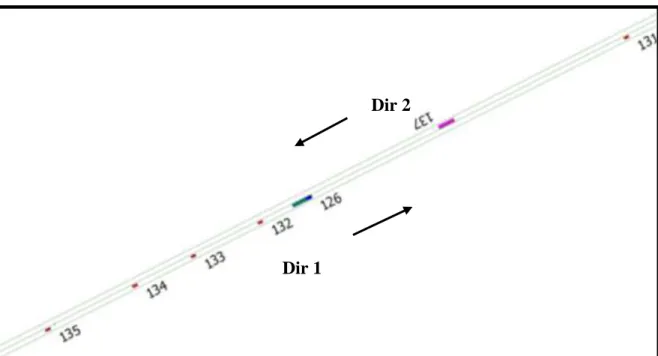
(11) 3.3.. Model Calibration ........................................................................................................ 31. 3.3.1.. Calibration of Traffic Simulation Models ............................................................ 32. 3.4.. Model Validation ......................................................................................................... 33. 3.5.. Verification and Validation Techniques ...................................................................... 33. 3.6.. Statistical Hypothesis Test ........................................................................................... 35. CHAPTER 4 ..................................................................................................................................... 37 VERIFICATION OF THE NEW VERSION OF RURAL TRAFFIC SIMULATOR ........................................ 37 4.1. The verification Plan .................................................................................................... 37. 4.2. Study Site ..................................................................................................................... 37. 4.3. Available Input Data .................................................................................................... 38. 4.4. Road Design ................................................................................................................. 39. 4.5. Model Simulation Runs ............................................................................................... 40. 4.6. Model Verification and Validation .............................................................................. 41. CHAPTER 5 ..................................................................................................................................... 42 SIMULATION RESULTS AND ANALYSIS .................................................................................... 42 5.1. Verification of Free vehicles ........................................................................................ 42. 5.2. Verification of the model run with interactions ........................................................... 44. 5.2.1. Animation review ................................................................................................. 44. 5.2.2. Speed comparison ................................................................................................. 45. 5.2.3. Constrained vehicles comparison ......................................................................... 47. 5.2.4. Travel time comparison ........................................................................................ 48. 5.2.5. Number of overtaking comparison ....................................................................... 49. 5.2.6. Traffic flow comparison ....................................................................................... 52. 5.2.7. Speed flow relationships ....................................................................................... 52. 5.3. Hypothesis Test Analysis ............................................................................................. 53. CHAPTER 6 ..................................................................................................................................... 56 CONCLUSION AND FUTURE WORK ................................................................................................ 56 6.1.. Discussion and Conclusion .......................................................................................... 56. 6.2.. Future Work ................................................................................................................. 57. REFERENCES ................................................................................................................................... 59 APPENDICES ................................................................................................................................... 64 Appendix A: Traffic flow compositions at RV51-Örebro ..................................................... 64.

(12) Appendix B: Model parameter values .................................................................................... 65 Appendix C: Average speed comparison in the two simulators ............................................ 67 Appendix D: Speed flow relationship .................................................................................... 70 Appendix E: Comparison between the simulation results and the field measurements ......... 74 Appendix F: Hypothesis test results ....................................................................................... 77.

(13) List of Figures Figure 1: RuTSim flow chart (Tapani.A., 2005) ............................................................................ 12 Figure 2: Notations of vehicle movement ...................................................................................... 16 Figure 3: Traffic micro-simulation model development process (FGSV Verlag GmbH , 2006). . 27 Figure 4: Study site at Örebro; Riksväg 51 .................................................................................... 38 Figure 5: Screenshot of the modeled road in RuTSim 2 ................................................................ 40 Figure 6: Number of overtakings vs. traffic flow per direction ..................................................... 51 Figure 7: Maximum sight distance information ............................................................................. 51 Figure 8: Speed flow relationship for cars in direction 1 ............................................................... 53 Figure 9: Speed flow relationship for cars, in direction 1 .............................................................. 70 Figure 10: Speed flow relationship for bus/trucks in direction 1 ................................................... 70 Figure 11: Speed flow relationship for truck 34 in direction 1 ...................................................... 71 Figure 12: Speed flow relationship for truck 5 in direction 1 ........................................................ 71 Figure 13: Speed flow relationship for cars in direction 2 ............................................................. 72 Figure 14: Speed flow relationship for bus/trucks in direction 2 ................................................... 72 Figure 15: Speed flow relationship for truck 34 in direction 2 ...................................................... 73 Figure 16: Speed flow relationship for truck 5 in direction 2 ........................................................ 73. List of Tables Table 1: Traffic volumes in each direction, RV51-Örebro ............................................................ 39 Table 2: Speed limits at different position of the road section ....................................................... 40 Table 3: Free flow speed comparison between the two simulators, RV51-5 ................................. 43 Table 4: The measured average speed for free vehicles................................................................. 43 Table 5: Comparison between the simulation free flow speed and the field, RV51-5 .................. 44 Table 6: Speed comparison between the simulators before verification, RV51-1 ......................... 45 Table 7: Speed comparison between the two simulators after the model is corrected, RV51-1 .... 46 Table 8: 95% prediction intervals of the simulated average speed measurements, RV51-1 ......... 47 Table 9: Percentage of constrained vehicles .................................................................................. 48 Table 10: Comparison of travel time of the cars ............................................................................ 49 Table 11: Comparison between number of overtakings and catch-ups.......................................... 50 Table 12: Comparison of simulated traffic flows with traffic flows from field measurements presented as 95% prediction intervals ............................................................................................ 52 vii.

(14) Table 13: Hypothesis test results of the average speed and the standard deviation, RV51-1 ........ 54 Table 14: Hypothesis test result of the travel time for cars ............................................................ 55 Table 15: Traffic flow composition in both directions Nordlöf, M., & Onmalm, L. (2006) ......... 64 Table 16: Average speed comparison between the two simulators, RV51-1................................. 67 Table 17 Average speed comparison between the two simulators, RV51-2 .................................. 67 Table 18: Average speed comparison between the two simulators, RV51-3................................. 68 Table 19: Average speed comparison between the two simulators, RV51-4................................. 68 Table 20: Average speed comparison between the two simulators, RV51-5................................. 69 Table 21: Average speed comparison between the two simulators, RV51-6................................. 69 Table 22: 95% prediction intervals of the simulated speed measurements, RV51-1 ..................... 74 Table 23: 95% prediction intervals of the simulated speed measurements, RV51-2 ..................... 74 Table 24: 95% prediction intervals of the simulated speed measurements, RV51-3 ..................... 75 Table 25: 95% prediction intervals of the simulated speed measurements, RV51-4 ..................... 75 Table 26: 95% prediction intervals of the simulated speed measurements, RV51-5 ..................... 76 Table 27: 95% prediction intervals of the simulated speed measurements, RV51-6 ..................... 76 Table 28: Hypothesis test results of the average speed and the standard deviation, RV51-1 ........ 77 Table 29: Hypothesis test results of the average speed and the standard deviation, RV51-2 ........ 77 Table 30: Hypothesis test results of the average speed and the standard deviation, RV51-3 ........ 78 Table 31: Hypothesis test results of the average speed and the standard deviation, RV51-4 ........ 78 Table 32: Hypothesis test results of the average speed and the standard deviation, RV51-5 ........ 79 Table 33: Hypothesis test results of the average speed and the standard deviation, RV51-6 ........ 79. viii.

(15) CHAPTER 1 INTRODUCTION 1.1. Introduction. Transportation plays a vital role for the socio economic aspects all over the world. Therefore, any problem in transportation systems can have a great impact on all economic activities and social well-being. Thus, a traffic planner should give attention to avoid possible problems that occur in transportation systems. In the last years, traffic and transport demand have increased at a high rate which results in capacity problems in the infrastructure, causing traffic jams and delays (Burghout, 2004). Currently, congestion and traffic jams are common problems in transportation networks. To facilitate well-functioning traffic and transportation systems, a traffic planner needs traffic models which can predict the influence of the road design, increased travel demand and introduction of traffic management systems. Traffic models are important tools for modeling the operations of traffic systems and to analyze the causes and possible solutions of traffic problems such as congestion, traffic jams, delays and traffic safety. Researchers have developed different types of traffic simulation models to analyze the problems in transportation systems and propose possible solutions. Traffic simulation models can be classified as macroscopic, mesoscopic and microscopic based on the level of detail at which they represent the traffic stream. Macroscopic simulation models represent the traffic stream and interactions at a low level of detail and they are capable of simulating large traffic networks. The level of details in mesoscopic simulation models lies between Macro and Micro simulation models. Mesoscopic traffic models represent the traffic stream at a higher level of detail but at a lower level of detail with respect to the modeling of interactions. Microscopic simulation models represent the traffic stream at a high level of detail and simulate individual vehicles. This master’s thesis focus on microscopic traffic simulation models for rural roads. As mentioned earlier, traffic simulation models have become very important means for analyzing real-world transportation problems. With the quick development of technology, several traffic simulation models have been implemented. In order to have a successful traffic simulation model, 1.

(16) the ‘correctness’ or ‘credibility’ of the model is fundamental and several testing processes must be performed to ensure the quality of the simulator before the simulation model is applied to real problems. Model verification, calibration and validation are very important phases in the development of a simulation model and they are also considered to be parts of the model development process, see further discussion in connection with Figure 3 in chapter 3. The following six stages should be considered in the model development process: Framework: In the first stage, the developer should construct the model framework, i.e., the model inputs and outputs, etc. Specification: the model framework described in the first stage is specified in a more detailed way. For example; in traffic simulation model, the car-following model or other sub-models going to be used in the model is specified in this step. Implementation: is the process of implementing the model in a software program. Verification: is a process of testing the simulation model in order to examine whether the model is programmed correctly or not. This process includes debugging software, looking for incorrect implementation of the code, and verifying the calculations (Xiang, et al. 2005,). Calibration: is the process of adjusting the model parameters in order to reproduce the realworld system. Field data should be available to perform model calibration. Validation: is the process of evaluating the model by using real field data. If the result of the validation is not applicable, it indicates that some input parameters should be adjusted i.e., there is a need to go back to the calibration so that the model can reproduce the real-world system. Sometimes it might also be required to go back to the verification process. Therefore, verification is strongly recommended before the model is applied or used to analyze real world cases. The model developer is responsible for the verification and validation processes (Rakha, et al. 1996). However, when applying a model for a specific real-world problem further calibration and validation to the local condition must be performed. The verification, calibration and validation processes are discussed in chapter 3 in detail. 2.

(17) 1.2. Problem Statement and Aim of the Thesis. A new version of the Rural Traffic Simulator, RuTSim has been implemented mainly based on the earlier one but with some enhancements. For instance, the intersection and the car-following models have been improved in the new implementation. The implementation of the new intersection model has implied a restructuring and partly new implementation of the behavior models describing and simulating driver’s behaviors on road links between intersections. This reconstruction and new implementation requires that a new verification and calibration to be conducted. The aim of this master’s thesis is to conduct a verification of the new implementation of the RuTSim model, investigate a good way of doing model verification and compare the result of the new implementation with the old version of the RuTSim model, since the old version is well verified and validated (Tapani, 2005, 2008). If there are significant differences between the two results, reasons for the differences have been investigated. Minor validation will be also conducted for the new version of the RuTSim model, since the speed measurements from the field are available. 1.3. Delimitations. RuTSim has the capacity to simulate all common rural highways including intersections and roundabouts of the main road traffic. The first limitation of this study is that, the verification focuses only on the link model, i.e., the verification of the new intersection model is not included in this thesis as an upcoming study is conducting on the verification of the new intersection model. Another limitation is that the thesis only considered normal two- lane rural roads with oncoming traffic. 1.4. Methods. The methods to be followed in the verification of the rural traffic simulator, RuTSim are: -. Literature study on traffic simulation models, particularly traffic simulation models for rural highways, and verification of traffic simulation models.. -. Theoretical assessment of the different verification schemes. 3.

(18) -. Investigate and select a good way of performing verification, i.e., define which road types, traffic measurements, vehicle type compositions etc. that should be simulated and investigated.. -. Perform verification of the new implementation of the RuTSim model. -. Result analysis. -. Compare the result of the new implementation with results from the old version of the RuTSim model. -. Statistical hypothesis test in order to check if any changes in the measurement of effectiveness are statically significant or not.. 1.5. Discussion and Conclusion Structure of the Thesis. This thesis report consists of 6 chapters. Microscopic traffic simulation models particularly the Rural Traffic Simulators (both the new and the old versions) are introduced in chapter 2. Chapter 3 presents the literature review on verification, calibration and validation techniques of simulation models. Chapter 4 presents a brief discussion on the input data used in the model simulation and model verification plans. The simulation results of the two simulators, both the old and the new versions of the RuTSim model is discussed briefly in chapter 5. Finally, conclusion and future work is presented in chapter 6.. 4.

(19) CHAPTER 2 MICROSCOPIC TRAFFIC SIMULATION MODELS This chapter gives an introduction to microscopic traffic simulation models followed by a brief discussion on one of the microscopic traffic simulation models for rural roads, the Rural Traffic Simulator, RuTSim. 2.1.. Behavior Models of Microscopic Traffic Simulation Models. Microscopic traffic simulation models, also known as traffic micro-simulation models, simulate individual vehicles, and the interaction between vehicles and with the road infrastructure. Traffic micro-simulation models include some rules of behavior that controls the movements of the vehicles, e.g. how and when the vehicles decelerate, accelerate, change lane, overtake, etc. Behavioral models, sub-models of traffic micro-simulation models, commonly include car following, lane changing, gap acceptance, overtaking, speed adaptation, and ramp merging. All traffic simulation models do not require all the sub-models at once. The required sub-models to be used depend on the type or the purpose of the traffic simulation. For instance, lane changing models are not necessary for rural road traffic simulation models of two-lane highways with oncoming traffic but they are essential for simulation of freeways and urban road traffic. Among the sub-models the most important one is the car-following model, and it is common for both rural and urban traffic simulation models (Olstam, 2009). The sub-models of traffic microsimulation models are discussed in detail in the following sub sections. Micro traffic simulation models can use a time based scanning approach or an event based approach. In a time based approach, the simulated vehicles are updated according to the behavior of the sub-models at a regular time interval. The simulation time step in this approach is constant and usually in between 0.1 - 1 second, whereas in event based approach, the vehicles are updated when the state of the system entities is changed. Some examples of traffic micro-simulation models for freeways and urban roads are, AIMSUN (Barceló, 2010, TSS, 2012), VISSIM (PTV 2008), Paramics (Quadstone Paramics, 2012), MITSIMLab. (Toledo,. T.. et. al.,. 2003),. and. CORSIM. (FHWA. 1996).. Whereas,. traffic micro-simulation models for rural roads include the Two-Lane Passing, TWOPAS (Leiman et al., 1998), the Traffic on Rural Road model, TRARR (Hoban et al., 1991), the 5.

(20) VTISim model (Brodin and Carlsson, 1986) and CORSIM (Washburn et.al., 2010). The focus of this thesis, the Rural Traffic Simulator (RuTSim) (Tapani, 2005, 2008), has been developed based on VTISim. 2.1.1. Car Following Models The car-following model controls the acceleration of a simulated vehicle based on the speed of the vehicles in front on the same lane. It is crucial for all types of road environments. The speed of a front vehicle is not dependent on the following vehicles, but the speed of a following vehicle is dependent on the speed of the front vehicles. A vehicle can be described as: i.. Following: when the speed of the vehicle is dependent on the speed of vehicles in front, hence, the vehicle cannot drive at its desired speed.. ii.. Free: when the vehicle is not forced to follow the speed of vehicles in front, hence the speed of the vehicle is mostly the same as its desired speed (Olstam, 2009).. 2.1.2. Lane Changing Models The lane changing model is essential for traffic micro-simulation models. It is applicable for roads with more than two lanes in the same direction. A lane changing model controls the behavior of a driver deciding whether to change lane or not. In the lane changing process the following three factors should be considered: -. Possibility (Is it possible to change lane?). -. Necessity (Is it necessary to change lane?). -. Desirability (Is it desired to change lane?). The lane changing model developed by Gipps (1986) is based on the above three lane changing decisions. It states that lane changes are not possible unless the gap in the target lane is acceptable. However, if it is mandatory to change lane, vehicles in the target lane will adjust their acceleration in order to create an acceptable gap and to help the vehicle to change lane. Based on the above three lane changing decisions (the Gipps model) different lane changing models have been developed, such as; Barceló and Casas (2002), Hidas (2002, 2005), Yang (1997). All of them are discussed in Olstam (2009) in detail.. 6.

(21) Lee (2006) suggested that the following three steps should be considered in modeling of the lane changing process,. decision,. (ii) selection, and. (iii) gap acceptance. CORSIM. (Halati et al., 1997) is one of the traffic micro-simulation models, which classifies the lane changing as mandatory or discretionary. Mandatory lane changing occurs when the current lane is not available and the driver has to change lane to reach his/her destination. Whereas, in discretionary lane changing the driver wishes to change lane in order to pass a vehicle in front. As described earlier, lane changing models are not that necessary for rural roads and two-lane highways with oncoming traffic. But it is important for urban roads and freeways. 2.1.3. Gap Acceptance Models The gap acceptance model is a part of lane changing models (intersection and overtaking models as well) and it is an important sub-model in traffic micro-simulation models. A gap acceptance model checks the gaps between two succeeding vehicles when lane changing process is taking place. The word gap by definition refers to the time or the space required by a vehicle to change lane safely. Therefore, the gap acceptance model is used to assess whether the gap between vehicles is acceptable by a driver to change lane or not. In principle the driver should check only the adjacent gap, the distance between lead (front) vehicle and a lag (following) vehicle. If the adjacent gap (both the lead and the lag gaps) is acceptable by the driver then the driver can change lane immediately. The critical gap in the gap acceptance model is the most important parameter to take into consideration. The critical gap is the minimum time gap that a vehicle that wants to change lane would accept to enter to its target lane. Lee (2006) formulated the gap acceptance as a binary choice as shown below: ,. (2.1). where; -. is the choice indicator variable,. -. is the current available gap. -. is the critical time gap. When the available gap is less than the critical one, the driver rejects the gap and fails to enter the targeted lane. If the available gap is greater than the critical gap then the driver accepts the gap, (Hwang, et al. 2005). 7.

(22) 2.1.4. Overtaking Models The overtaking model controls the behavior of vehicles when they desire to overtake and when the overtaking process is taking place. Before overtaking the driver should consider the following four overtaking decisions: -. Overtaking restrictions: the driver should check if there are overtaking restrictions within the near distance from the position of the vehicle. For instance, restrictions allocated at 300 meter away from the position of the vehicle can be assumed to not affect the overtaking decision, (Olstam, & Tapani, 2004).. -. The given available gap: the driver should check if the available gap in the oncoming traffic stream is big enough to perform the overtaking.. -. Performance of the vehicle: the vehicles need to be able to pass the vehicle in front in a reasonable time and distance. The performance of the vehicles can be assessed with the overtaking distance and the desired speed differences between the two vehicles, i.e., the overtaking and the overtaken vehicles. This is further explained in section 2.3.3. -. The driver’s willingness: the driver’s willingness to perform an overtaking at the given available gap. The available gap is the distance to the first oncoming vehicle. Like gap acceptance in the lane changing model, the easiest way to model the gap acceptance in an overtaking model is to use a common critical gap for all drivers. But gap acceptance in an overtaking model needs to be more advanced than the gap acceptance in the lane changing case since the driver’s willingness to reject and accept the current gap differs among the drivers, (Olstam, 2009).. 2.1.5. Speed Adaptation Models A speed adaptation model is important for both urban and rural roads. Traffic micro-simulation models use model parameters to express the desired speed of a vehicle. Factors that affect the desired speed of a vehicle in rural roads differ from that of urban roads or freeways. For instance, in rural roads the desired speed is dependent on the geometry of the road (such as, road width, curvatures, grades, speed limit, etc.) to a higher degree than on urban roads where it is mainly dependent on the speed limit. Therefore, a speed adaptation model is needed to adjust the vehicle. 8.

(23) speed with respect to speed limit, curvatures and other road infrastructure related measures in rural roads. Tapani, (2005, 2008) describe how the basic desired speed of a vehicle can be reduced with respect to road width, horizontal curvature and speed limits. In the RuTSim model the basic desired speed is adjusted for road width, horizontal curvature and speed limits. See section 2.3.1 for further details. 2.2.. Microscopic Traffic Simulation Models for Rural Road Environments. Most microscopic traffic simulation models are designed for freeways and urban roads (Olstam, 2009). The requirements needed to develop a traffic model for urban roads or freeways differ from model development for rural roads. Traffic flows are different in rural and urban roads, and the vehicle-vehicle and vehicle-infrastructure interactions are different on these types of roads. For instance, the travel time delay on urban roads or freeways mainly depend on the interaction of the vehicles with each other, while the travel time delay on rural highways depend, to a higher degree, on the vehicle-infrastructure interactions. The vehicle-vehicle interactions therefore have less impact on rural road highway compared to freeway and urban roads. Therefore, traffic models for rural roads should take into account the interaction between vehicles and the infrastructure in greater detail than traffic models for urban roads (Tapani, 2008). In rural road environments there may be intersections, and segments of multilane roads, but this thesis focuses only on two lane highways without any intersections. Rural road and freeway traffic simulations began in the 1960’s. The first simulators were modeled to simulate two-lane highway traffic, (Shumate and Dirksen in 1964). However, the rural road traffic simulation models in the 1960’s were limited by the computing powers that were available at that time. In the last decades, several rural road traffic simulators have been developed, e.g. the Traffic on Rural Roads model (TRARR) developed by Australian Road Research Board (Hoban et al., 1991), the Two-Lane Passing model (TWOPAS) developed by Midwest Research Institute (McLean, 1989), the CORridor-microscopic SIMulation Program, CORSIM (Washburn et.al., 2010), the VTI rural simulation model (VTISim) developed by Swedish National Road and Transport Research Institute (Brodin and Carlsson, 1986), and the Rural Traffic Simulator (RuTSim) developed at Swedish National Road and Transport Research Institute (VTI) (Tapani, 2005, 2008). 9.

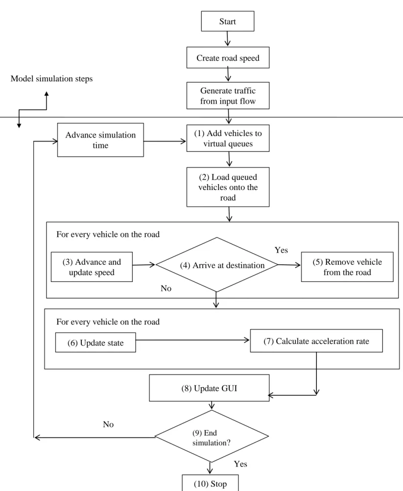
(24) 2.3.. The Current Rural Traffic Simulator, RuTSim 1. RUral Traffic Simulator, RuTSim, is a traffic micro-simulation model for rural roads and was developed at VTI (Tapani, 2005, 2008). The model is based on the VTI rural simulation model, VTISim. The model has capability to simulate all common types of rural roads including effects of intersection and roundabout on the main road network. The intersections can be with or without left turn lane. Vehicle entering the road network can leave at any time, i.e., it is possible to simulate interrupted traffic flow with the RuTSim model. However, the model is not intended to manage simulation of road networks; it handles only one road stretch in each simulation run. The model uses a time based scanning approach and the time step can be defined by the user. Tapani, (2005; 2008) pointed out the reason of using time based scanning approach is that it allows detail modeling of vehicle-vehicle and vehicle-infrastructure interactions. The shorter the time step, the smoother the movement of the simulated vehicles from one time step to the next, resulting in more accuracy. However, with the shorter time step, the simulation run time will be longer. During the simulation run the following steps are conducted at each time step. (See also Figure 1). But before the model simulation, one should create the road network and generate traffic volumes. 1. Add vehicles to virtual queues. One virtual queue is created for each origin. 2. If there is enough space available on the main road, load vehicles from virtual queued vehicles to the road. 3. Update speed and position for every vehicle on the road. 4. Check whether any vehicles have arrived at their destination or not. 5. If a vehicle has arrived at its destination, then remove it from the road. 6. For the vehicles that did not arrive at their destination, for every vehicle left on the road update their state, i.e. free or car-following, overtaking or passed, and acceleration rate. 7. Calculate the acceleration rate for every vehicle on the road 8. Save data and update the graphical user interface 9. If the simulation time ends up, then stop the simulation otherwise increase the simulation time and go back to the first step.. 10.

(25) The RuTSim model is capable of simulating the following road section types (Tapani, 2005). -. Normal two lane highways with oncoming traffic. -. Two lane highways including overtaking or climbing lanes. -. One lane section with a barrier between the oncoming lane. -. Transient two-lane section with a barrier between the oncoming lanes that will change into a one-lane section. -. Two-lane section with a barrier between the oncoming lanes and no indication of change in the number of lanes.. 11.

(26) Start. Create road speed Model simulation steps Generate traffic from input flow. (1) Add vehicles to virtual queues. Advance simulation time. (2) Load queued vehicles onto the road. For every vehicle on the road Yes (3) Advance and update speed. (4) Arrive at destination. (5) Remove vehicle from the road. No. For every vehicle on the road (7) Calculate acceleration rate. (6) Update state. (8) Update GUI. No (9) End simulation?. Yes (10) Stop Figure 1: RuTSim flow chart (Tapani.A., 2005) 12.

(27) The sub-models of RuTSim which are relevant for this study are discussed based on the description of the model in Tapani, (2005; 2008). 2.3.1. Speed Profile Model The speed profile model refers to the desired speed of a vehicle along the road. The model assigns a basic desired speed for each simulated vehicle. . And it is assumed to be normally. distributed based on the distribution with a median speed,. , which is a calibration parameter. (Tapani, 2005). The speed profile model will update the desired speed of each vehicle whenever the road geometry and the speed limit changes. As mentioned in section 2.1.5, the desired speed of a vehicle, speed. , is in RuTSim affected by the following three factors resulting in a final desired. .. -. Road width:. -. Horizontal curvature. -. Speed limit. Road width: For roads with a width between 7.5 m and 8.0 m, the median basic desired speed, , is reduced to. =. whereas, for roads with narrower than 7.5 m. is calculated as:. (2.2). where; -. is the road width in meter. -. is a model parameter, which is estimated to be 0.042. -. is a model parameter which is estimated to be 27.75 m/s. Horizontal curvature: the median desired speed reduced with respect to the road width, further reduced with respect to horizontal curvature, the median desired speed,. , can be calculated as:. 13. , is. . For curves with radius less than 1000 m,.

(28) (2.3). where; -. is the horizontal curve radius in meter. -. is a model parameter, which is estimated to be 0.15. Speed limit: the median desired speed reduced with respect to both road width and horizontal curvature,. , is again reduced with respect to speed limit to the final median desired speed,. ,. which is calculated as: (2.4). where; -. is the current speed limit in km/h is a model parameter, estimated to be 0.050 is a function of the speed limit, defined as: (2.5). Each desired speed, which is reduced with respect to the above three factors, is tested with different values of its corresponding model parameters and discussed in detail in (Tapani, 2005). As mentioned earlier, the desired speeds are normally distributed. The distribution dispersion is characterized by a dispersion measure,. . The desired speed of a. vehicle at any point on the road is calculated as: ,. (2.6). where; -. is a vehicle type dependent model parameter, in between 0 and 1, for cars it is set to 0.. -. is the desired speed of a vehicle/car with respect to road geometry and speed limit. -. is the basic desired speed of vehicle. In the RuTSim model (Tapani, 2005), the dispersion measure , of the desired speed distribution is calculated as a weighted average of the dispersion measure of the desired speed with respect to 14.

(29) road width, horizontal curvature and speed limit, denoted as. ,. , and. respectively.. is. calculated as: (2.7) where. ,. , and. are the weights with respect to road width, horizontal curvature and speed. limit respectively and can be obtained by using the following expressions: (2.8) (2.9) (2.10) If. =. =. If the value of. = 0, then. =1. is less than 1, then it indicates that a vehicle with high basic desired speed will. decrease its speed more than a vehicle with a lower basic desired speed. The above three expressions, eq (2.8), (2.9) and (2.10) show that the speed limit has greater effect on the dispersion measure than horizontal curvature and that horizontal curvature has greater effect than the road width on the dispersion measure. 2.3.2. Acceleration Model The acceleration sub model in RuTSim consists of the following parts: -. Acceleration with respect to the road geometry. -. Acceleration with respect to constraining vehicles. The following figure will help to understand the notations used in the acceleration model description (Tapani, 2005).. 15.

(30) Figure 2: Notations of vehicle movement. Acceleration with respect to the road geometry It has been mentioned that the basic desired speed is dependent on road width, horizontal curvature, and speed limit. Free vehicles are assumed to be traveling with their desired speed. If the current speed of a vehicle. is less than the desired speed, the acceleration rate is computed. as: (2.11) where; -. is the power to mass ratio of vehicle. -. ,. -. is the acceleration due to gravity.. -. , and. measured at the wheels.. are air and rolling resistance coefficients. is the vertical grade at the position of vehicle is speed of a vehicle. If the current speed of a vehicle is higher than the desired speed, the deceleration rate is computed as. (2.12). The above two expressions represent a deceleration rate with engine and downhill, and with decelerator pedal,. , which is used to balance the acceleration due to gravity. 16. ,.

(31) Acceleration with respect to constraint vehicles The car-following model of a microscopic traffic simulation model has been described in section 2.1.1. A vehicle which follows a slower vehicle is considered to be a following vehicle; hence the speed of a following vehicle is dependent on the speed of the preceding vehicle. The following vehicle will be forced to decelerate in order to adjust its speed with respect to the speed of the preceding vehicle. A vehicle behind a faster vehicle is considered to be free. A vehicle that follows a faster vehicle has opportunity to accelerate in order to catch up with the preceding vehicle. The acceleration rate in this condition is given by an asymmetrical GHR model (Yang and Koutsopoulos, 1996):. (2.13). where; sign if. ,. , and. are model parameters. The plus sign is used if. and the minus. .. If the acceleration computed with respect to car-following is larger than the acceleration computed with respect to road geometry, then the follower vehicle takes the later, i.e., the acceleration computed with respect to the road geometry. If the distance to the preceding vehicle is shorter than the desired one and the speed of the preceding vehicle is lower than the speed of the following vehicle then the following vehicle should decrease its speed in order to create a safe gap to the preceding vehicle and avoid collision. The deceleration rate in this condition is calculated as: .. (2.14). 2.3.3. Overtaking Model The overtaking model, as described earlier, controls the behavior of vehicles when they want to overtake and when the overtaking process is taking place. Overtaking behavior differs in different road types. In this section only the overtaking behaviors on normal two lane sections with oncoming traffic is presented. The overtaking model used in such type of road is based on the overtaking model in VTSim (Tapani, 2005).. 17.

(32) Two types of overtaking take place on two-lane sections with oncoming traffic. These are flying and accelerated overtaking. Flying overtaking refers to when a vehicle decides to overtake a slower vehicle; that is the speed of a following vehicle is greater than the speed of the preceding one. The overtaking is possible only at the time when the following catches the preceding. If it is impossible to perform a flying overtaking then the following vehicle adjusts its speed to the preceding and later, when it is possible, the following vehicle might accelerate to perform an overtaking. This type of overtaking is referred to as accelerated overtaking. The following vehicle has opportunity to perform an accelerated overtaking when the sight distance reaches a maximum. In case the overtaking opportunity of the following vehicle is not accepted because of oncoming vehicles within sight distance, the following vehicle will get another opportunity after the oncoming vehicle has passed. Overtaking decisions considered in the RuTSim model are the same as the overtaking decisions that have been described in section 2.1.4, i.e., overtaking restrictions, the possibility to perform overtaking considering the surrounding traffic situation, performance of a vehicle, and the driver’s willingness. Vehicles cannot perform an overtaking if there are overtaking restrictions within the area. However, the overtaking restrictions allocated 300 meters away from the position of a vehicle can be assumed not to affect the decision, (Olstam, 2004). Before performing overtaking, the driver should take into account the surrounding traffic. For instance overtaking is not allowed if: -. a vehicle is being overtaken.. -. a vehicle is preparing to exit the road by making a left turn. -. there is no large enough gap. Overtaking can be also given up if the overtaking vehicle cannot travel faster than the one to be overtaken. The performance of a vehicle to perform an overtaking can be assessed with the overtaking distance and the desired speed difference between the two vehicles, the overtaking and the overtaken vehicles. The desired speed difference should be greater than the minimum allowed desired speed and the overtaking distance should not be longer than the maximum allowed. 18.

(33) distance which is assumed to be 1000 meters. The overtaking distance for flying and accelerated overtakings can be estimated by the following two expressions respectively. (2.15). (2.16). where; -. is the maximum acceleration of the overtaking vehicle obtained by eq (2.13). -. is the overtaking distance which a vehicle should travel comparative to the overtaken vehicle, which is calculated as: (2.17). Gompertz functions have been used to describe the driver’s willingness to perform overtaking as a function of the available sight distance. The probability to perform overtaking is calculated as. (2.18). where; -. is the overtaking probability with a given a clear sight distance. -. is the threshold for the minimum clear sight distance for accelerated or flying overtaking.. -. and. are parameters and have different values for different combination of road widths,. types of overtaking, overtaken vehicles, and sight limiting factors. The probability given by eq (2.18) is reduced using eq (2.19) if the vehicle ahead is a part of a platoon. (2.19) where; -. is the number of vehicles in the platoon ahead is the parameter controlling reduction per vehicle in platoon. 19.

(34) 2.4.. Traffic Generation. The traffic generation process in the RuTSim model includes the determination of origin and destination of a vehicle, speed of a vehicle, entry time, and assignment of individual vehicle parameters. The RuTSim model includes individual driver/vehicle characteristics which can be static or dynamic. Vehicle parameters that can be changed during simulation are referred to as dynamic, whereas vehicle parameters that cannot be changed during simulation are referred to as static. Static and dynamic vehicle characteristics have been listed in (Tapani, 2005). The traffic generation model consists of four types of vehicles. These are: car, truck and bus, truck with trailer, and truck with semi-trailer. The RuTSim model uses a platoon generation model with the purpose of reducing the warm up stretches which are required until stable traffic flow is produced. Platoons of vehicles for the current traffic volume and compositions are created by the platoon generation model. The platoon length is calculated as: (2.20). , where;. is the average platoon length and the value of Z is given by:. ,. where;. and. direction.. (2.21). in are denoted the traffic volume and the overtaking possibility in the current. is calculated as: ,. (2.22). where; -. and. are model parameters which represent the road standard and the average time. gap between vehicles respectively. -. and. are obtained from input data, and they are representing the traffic volume in. the opposite direction and the composition of heavy vehicles in the current flow respectively.. 20.

(35) 2.5.. Model Inputs and Outputs. 2.5.1. Input Data The main required input data for the RuTSim model includes road data and traffic data. The traffic volume (vehicles per hour) and the traffic composition should be specified for both directions. Input data that can be specified in the RuTSim model are: Road data: -. Road length. -. Road standard. -. Speed limit profile. -. Road width profile. -. Horizontal curvatures profile. -. Vertical incline profile. -. Auxiliary lane profile. -. Restrictions on overtaking profile. -. Sight distance profile. -. Intersection coordinates and type. Traffic data: -. Traffic flows. -. Traffic composition. -. Start and end time of the simulation. -. Vehicle parameters (such as, P value (power to mass ratio), length and width of a vehicle, desired speed, etc…). -. Vehicle and driver settings (such as, maximum reaction time, minimum time head way, maximum deceleration, etc…). -. Simulation control parameters. 2.5.2. Outputs Available outputs obtained from a simulation run include aggregated traffic performance and individual vehicles driving course of events (can be used as input to pollutant emission models). The outputs are given as a text file and can be edited by external data analysis tools (e.g. Notepad++ editor) for further data analysis. The simulation output can be specified for points and. 21.

(36) sections. This should be specified before the simulation runs. The following aggregated traffic measures are available as a simulation result for the selected points along the road. -. Number of vehicle observations for each vehicle type.. -. Distribution of point speeds for each vehicle type.. -. Constrained percentage of vehicles per vehicle type.. -. Total number of platoons and distribution of platoon lengths.. The section data is aggregated into the following traffic measures -. Number of vehicle observations for each vehicle type.. -. Journey speed distributions for each vehicle type.. -. Average percentage of travel time and travel distance spent as constrained by a preceding vehicle.. -. Overtaking rates and densities for light and heavy vehicles. -. An average meter-by-meter driving course of events per vehicle type which consists of time, speed, acceleration and percentage of free driving vehicles.. 2.6.. The New Version of Rural Traffic Simulator, RuTSim 2. The new version of RuTSim was implemented based on the earlier version but with some improvements in the car-following model, overtaking model and the intersection model. The new intersection model is implemented based on the intersection model developed in the licentiate thesis by Strömgren (2002). The intersection model will be described and verified in the upcoming PhD thesis work by Per Strömgren; hence the description of the new intersection model has not been included in this report. The new car-following model is described below based on the model description in Olstam (2009). 2.6.1. Acceleration The new version of RuTSim uses a time continuous car-following model, which is known as the Intelligent Driver Model, IDM, (Treiber et al. 2006). The car-following model, as described in section 2.1.1, controls the acceleration of a simulated vehicle based on the speed of the preceding vehicles on the same lane. Desired speed, desired time gap, desired maximum acceleration rate and desired deceleration rate are model parameters included in the IDM car-following model. The acceleration of a vehicle is determined as:. 22.

(37) (2.23). where; is the free acceleration of the vehicle. It is dependent on the vehicle’s desired speed. -. and acceleration capability. -. is the interaction acceleration used in order to keep a safe distance to the preceding vehicle. -. is the distance headway. -. is the current speed of the vehicle and. -. is the speed difference between the vehicle and the preceding vehicle.. The free acceleration and the interaction acceleration of a vehicle are obtained from the following two expressions respectively. (2.24). (2.25). In eq (2.24), -. is the vehicle desired speed, and a parameter which determines the maximum acceleration.. In the interaction acceleration equation, eq (2.25), -. ,. ,. ,. -. is the parameter which controls the gap ratio. -. and. , and when. are the actual and the desired safety gaps respectively,. . is calculated as: (2.26). 23.

(38) where,. ,. ,. are model parameters which determine the minimum distance between. stationary vehicles, the desired following time gap and the desired maximum deceleration rate respectively. The IDM car-following model can also be extended with the Human Driver Model, HDM (Treiber et al., 2006) in order to model the human drivers’ behaviors in a more realistic way. In HDM, the acceleration of a vehicle is calculated as follows:. (2.27). where; -. is the current time. -. is the reaction time of the driver-vehicle unit , and. -. is the number of vehicles in front taken in consideration. However in RuTSim n = 3 is currently used.. Overtaking As discussed in section 2.3.3, the overtaking model used in the current version of RuTSim (RuTSim 1) is based on the overtaking model in the VTSim model. During overtakings, the driver should take the distance to the oncoming vehicle in the opposite lane and the remaining distance of the overtaking in to consideration. Therefore, the overtaking model is improved with a decision rule on abortion of overtakings. This decision rule stated as follows in Olstam, (2009). “A driver takes action if the time to collision, TTC with the oncoming vehicle is less than the estimated time remaining for the overtaking. Thus, if TTC + is a safety margin and. <. where. is the estimated time remaining for the overtaking.”. The time remaining for the overtaking is calculated as:. (2.28). where; -. ,. is the length of the vehicle. is the critical lag gap for lane changes to the right 24.

(39) -. is the time it takes to perform the lane change back to the normal lane is the acceleration of vehicle. and it is calculated based on eq (2.12) in section 2.3.2.. In eq (2.28), half of the lane change time is used since this time is assumed to be enough to clear the coming vehicles in the opposite lane and avoid collision with the oncoming vehicles. If the time remaining for the overtaking,. is greater than the time to collision, TTC, then the driver. should give up the overtaking. Since there are some enhancements in the new version of RuTSim, it should be verified in order to ensure that for a given input value the model gives a reliable output with the same argument which the program code is built. The general concept of verification, calibration and validation is discussed in the next chapter followed by verification of the new version of the RuTSim model.. 25.

(40) CHAPTER 3 VERIFICATION, CALIBRATION AND VALIDATION ASSESSMENT This chapter presents a brief discussion on three stages of the model development process: verification, calibration, and validation. 3.1.. Introduction. A simulation model by definition is an abstraction which represents the real-world system and it is built for the aim of analyzing real world problems. In the introduction section, it has been mentioned that verification, calibration and validation are stages in the model development process, see also Figure 3. Verification, calibration and validation are essential parts of the model development processes used to examine the correctness and the accurateness of the model. However, these processes cannot prove that the model is hundred percent accurate but they can give evidences that the model is adequately accurate or correct. Verification, calibration and validation are iterative processes, which mean that they will continue until the model is sufficiently accurate. Model verification refers to the processes of testing a simulation model weather the mathematical models are correctly implemented or not. A simple example, if a mathematical model states that z = x + y, then the verification examines if the computer model (program code) computes this mathematics correctly. Model calibration, on the other hand determines the best set of the input parameters in order to reproduce the real-world system i.e., the calibration process will stop when the simulation model can reproduce the real-world system sufficiently well. Model validation deals with the accuracy of the model by comparing the simulation result with another real data set which is not used during model calibration. The aim of model verification is to answer the question “Did we build the model right?” It is a process of checking and removing errors in the implemented model. On the other hand, model validation process answers the question “Did we build the right model? OR Is the model reliable?”. 26.

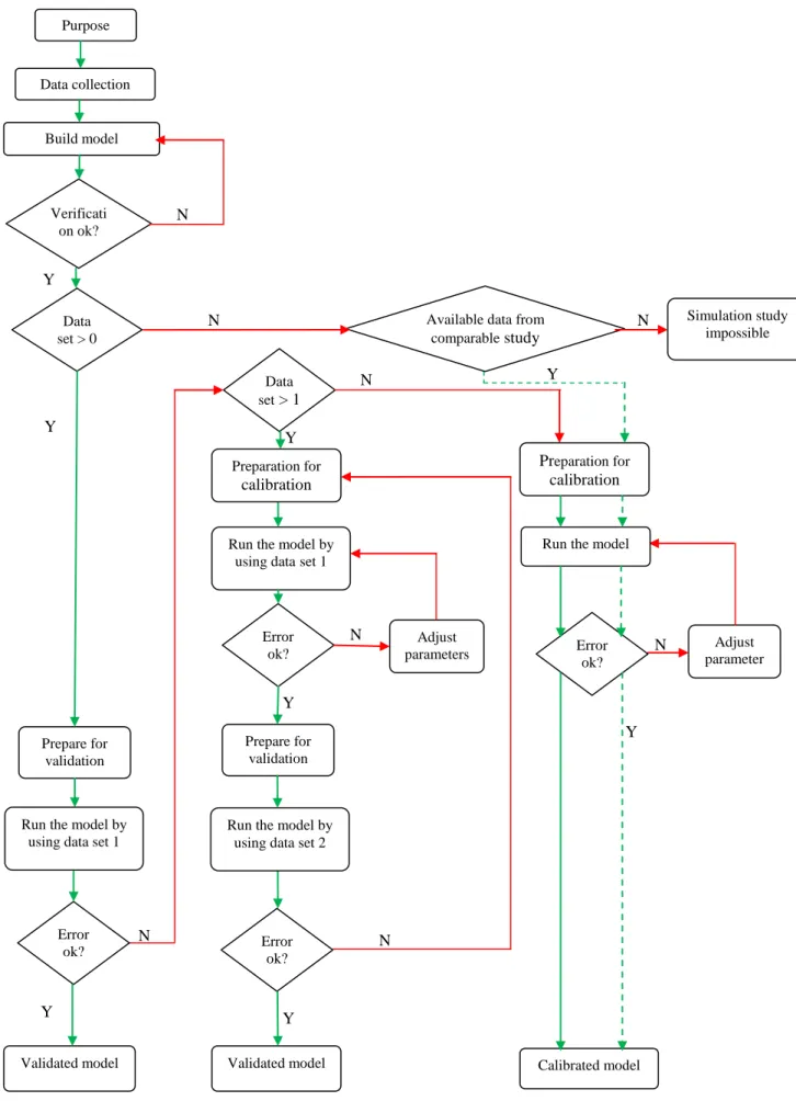
(41) Purpose. Data collection. Build model. Verificati on ok?. N. Y Available data from comparable study. N. Data set > 0. Data set > 1. Y. Simulation study impossible. N Y. N. Y Preparation for calibration. Preparation for. calibration. Run the model. Run the model by using data set 1. Error ok?. N. Adjust parameters. N. Error ok?. Adjust parameter s. Y Prepare for validation. Prepare for validation. Run the model by using data set 1. Run the model by using data set 2. Error ok?. Y Validated model. N. Error ok?. Y. N. Y Validated model. Calibrated model. Figure 3: Traffic micro-simulation model development process (FGSV Verlag GmbH , 2006). 27.

(42) 3.2.. Model Verification. As can be seen in Figure 3, after the model is built the next step is model verification. Model verification is the process of determining if the model implementation accurately represents the developer’s conceptual description of the model and the solution to the model, (AIAA 1998). It must be performed before the calibration and validation tasks so that the problems during calibration and validation processes can be avoided easily. It also helps to avoid wrong conclusions when performing calibration and validation tasks. Sargent, (2007) stated that the verification task can differ based on whether the model is implemented using a simulation language, or a higher level programming language (e.g., FORTRAN, C/C++, etc.). In a model implemented with a simulation language, the verification is focused on checking if the simulation language itself is error free and if the model has been programmed or implemented correctly. Whereas, in a model implemented in a higher level programming language, the verification task is focused on checking whether the simulation functions are well written or not, and ensures that the implementation of the computer model is correct. Both Thacker, et al (2004) and AIAA (1998) stated that the verification task can be classified as code verification and calculation verification. Code and calculation verification are defined as follow, AIAA (1998): 1. Code verification: identifies errors in the implemented code and check whether the mathematical model and solution algorithms are working correctly or not. 2. Calculation verification: identifies errors and check if the solution of the mathematical model is accurate. 1. Code verification Code verification is one of the verification tasks which identifies errors in the implemented code and tests whether the model is working as planned or not. The main purpose of this verification is to verify the accuracy of the model by finding and avoiding code errors which might happen during model implementation. Code verification activities are related directly towards the source code and the algorithm.. 28.

(43) Oberkampf, (2004) stated that the activities of code verification are to identify and remove errors in the source code and in the numerical algorithm, and to improve the software using software quality assurance verification techniques. Code verification is the responsibility of both model developer and code developer. Identifying and removing errors in the source code and in the numerical algorithm, referred to as numerical algorithm verification, which is the responsibility of the code developer. Software quality assurance, SQA, refers to testing the model to make sure that the code is implemented correctly and gives the same output on different operating systems and compilers; hence it is the responsibility of both model developer and code developer. 2. Calculation verification Calculation verification is carried out after code verification. Calculation verification is the process of identifying errors by comparing the result from the implemented code with those given by mathematical methods, referred to as numerical estimation error. Calculation verification can be done by both the user and the model developer but in principle it is the responsibility of the model developer (AIAA. 1998). When performing calculation verification, it is difficult to identify the numerical errors completely; the purpose of calculation verification therefore is to compute the accuracy of the model. Code to code comparison technique is one of the techniques in calculation verification. Performing code to code verification is difficult since it might not be easy to know which code is correctly implemented. The two codes may generate the same result; however, this does not indicate that the code to be verified is correctly implemented, since two codes can integrate the same error. Therefore, in code to code verification the code against which the new code is to be compared should be well verified in order to compute the correctness of the new code. The methods of code verification and calculation verification are discussed in detail in Woodward, (2011). 3.2.1. Verification of Traffic Simulation Models As mentioned earlier, the simulation output is not expected to be sufficiently accurate with the real traffic situation or the theoretical output. If the simulated output has major differences with the real traffic situation, the program code should be revised and corrected accordingly. During traffic simulation, a generated vehicle should reach its destination. Horiguchi, et al. (2002) stated that once a vehicle is generated, then it must not disappear until it reaches its destination. 29.

(44) Therefore, the verification process in generation of vehicles and flow conservation feature should verify if the generated vehicles in the simulation model reach their destination or not. It should also verify whether the number of generated vehicles in the model are equal to the given traffic volume or not. Horiguchi, et al. (2002) included the following six features in the Japan manual of standard verification process of traffic simulation models. Each feature has been discussed in detail in Horiguchi, et al. (2002). -. Generation of vehicles and flow conservation. -. Bottleneck capacity and saturation rate at link downstream end. -. Growing and shrinking traffic jam consistent with shock wave theory. -. Capacity of merging and diverging sections. -. Gap acceptance right/left turn at signalized intersection. -. Driver’s route choice behavior. Dowling, et al., (2004) and Vaughan, (2007) stated that verification of traffic micro-simulation model should be performed in three stages: checking, and. Software error checking,. Input coding error. Animation review. These three stages are discussed briefly as follows:. 1. Software error checking: is the process of checking whether the known bugs and workarounds in the software are taken into consideration with the latest version and patch of the software. 2. Input coding error checking: is the process of checking and removing errors from input data. Both Dowling, et al., (2004) and Vaughan, (2007) gave a brief explanation of checking the three categorized input data in microscopic traffic simulation models, these are; link and node network, traffic demand, and traveler behavior and vehicle characteristic. Link and node network: the users have to ensure that links in the road network and turning restrictions are defined correctly. Dowling, et al., (2004) described that static network display is also recommended to check the link geometry in the road network, (e.g. the numbers of lanes, the lane alignment, length, etc.).. 30.

(45) Traffic demand: the input volumes (turning volumes, O-D volumes) should be checked and compared to the collected field data in order to avoid unrealistic traffic flow and simulation result at the end. The traveler behavior and vehicle characteristics: includes checking the default value of vehicle performance specifications, vehicle types and vehicle dimensions. 3. Animation review: is the third stage and should be performed after the software and the input coding errors steps are conducted. It is the process of reviewing the animation of a simulation model to observe the movement of vehicles on the road network, which can help to identify errors which are not discovered in the above two stages. The process of reviewing animation of a simulation model can be conducted by running. the simulation model with. low demand level, so that the users can trace the movement of a vehicle in the network, and then. the simulation model with 50 percent of the total traffic volume in order to observe. the traffic congestion through the network, and check whether the traffic signals are correctly build up and at a right locations. As can be seen in the Figure 3, if the verification task is completed, then the model is run with the available data set. If the simulated result is not as expected, the next step is then to calibrate the model. Model calibration is discussed in the next section. 3.3.. Model Calibration. Once a simulation model is verified and if there is at least one datasets available, the next step is to validate and if necessary to calibrate the model. An initial validation is conducted in order to check if calibration is needed, see further discussion in Figure 3. Model validation is discussed briefly in section 3.4. Model calibration, as defined earlier, is the process choosing the best values of the input parameters. in. order. to. reproduce. the. real-world. traffic. systems.. All. traffic. micro-simulation models contain default values on the calibration parameters which are suggested by the model developer. Mostly, these values are unusual to reproduce the real traffic system for a particular area. Therefore, the users have to perform calibration in order to get sufficiently accurate result with the real traffic conditions. Thus, the purpose of model calibration is to select a best set of calibration parameters to reproduce the real traffic condition. The. 31.

(46) calibration task is performed by adjusting the input parameters and compare the output with the observed field data (here the accuracy level needed in the model should be taken into account). 3.3.1. Calibration of Traffic Simulation Models Both Dowling, et al., (2004) and Vaughan, (2007) have discussed the approach to calibrate traffic simulation models in detail and recommended three stages for conducting the calibration task. These are. capacity calibration,. route choice calibration and. system performance. calibration. Capacity calibration includes the adjustment of traffic capacity related calibration parameters in the simulation model so that the model can reproduce the traffic capacity in the field. In capacity calibration, only parameters that can affect the traffic capacity are calibrated. Global and local calibrations are two stages of capacity calibrations as stated by Dowling, et al., (2004). Global parameters related to traffic capacity are adjusted first and then local parameters are adjusted. An example of a global parameter related to traffic capacity is mean time headway. However, it may not have the same name in all simulation models. Route choice calibration includes the adjustment of the route choice parameters in order to reproduce field traffic flow. Route choice calibration has two stages: first global route choice parameters are adjusted and then link- specific fine-tuning (local) route choice parameters are adjusted. System performance calibration is the final stage of the calibration task as stated by Dowling, et al., (2004). It includes the adjustment of traffic performance parameters and the result is compared to the field measurements to evaluate the overall performance of the simulation model. Rakha, et al.,(1996) stated that there are two problems when conducting a calibration task. The first is, related to the quality and quantity of the field measurement data. As can be seen in Figure 3, to calibrate and validate the simulation model at least two different datasets are required, one for the calibration and another for the validation process. The second problem is that most users have faced it difficult to predict the simulation result of the changed parameters because of lack of knowledge on the simulation model and traffic theories. These dilemmas make the calibration task complicated. Therefore, to perform calibration task one should know the effect of the changed parameter on the output. 32.

No results found