GDP Elasticities of Export Demand : An analysis of Sweden’s export flows to Germany and other trading partners

(1)

GDP Elasticities of Export Demand

An analysis of Sweden’s export flows to Germany and other trading partners

Bachelor’s thesis within Economics

Authors: Mareike Bönninger 880914-5181 Camilla Nilsson 881106-4909 Tutors: Börje Johansson (Supervisor)

(2)

Bachelor’s Thesis in Economics

Title: GDP Elasticity of Export Demand Authors: Mareike Bönninger 880914-5181

Camilla Nilsson 881106-4909 Tutors: Börje Johansson (Supervisor)

Peter Warda (Deputy Supervisor)

Date: 2012-06-04

Subject terms: GDP elasticity of export demand, trade history, Sweden, Germany

Abstract

Exports are an important source of income for Sweden. They are influenced by macroeco-nomic factors such as GDP. This paper examines the elasticity of Swedish export to changes in the GDP of Sweden’s 25 most important export partners. The sensitivity to changes in GDP, the elasticity, can be different for different goods. Therefore, we examine export elasticities for five different commodity groups, which include durable as well as non-durable goods. Moreover, special focus is put on the trade relationship between Swe-den and Germany in order to see if their long common trade history has any impact on the elasticity of Swedish exports to Germany. The analysis is based on an export demand func-tion that links exports to GDP and geographical distance. We include dummy variables in our regression model to control for EU-membership and common borders.

For Swedish exports to Germany, we find that exports of food and live animals are least elastic, whereas exports of machinery and transport equipment are most elastic. This is co-herent with previous empirical findings about demand elasticities of non-durable and dura-ble goods. We find that exports in two out of five commodity groups are unit elastic. This means that when German GDP increases by one percent, Sweden’s export to Germany in these commodity groups also grows by approximately one percent. Thus, Sweden is not able to capture additional profit through over proportional increases in exports to Germa-ny. For Swedish exports to its 25 most important trading partners, on average, we find that exports of manufactured goods as well as machinery and transport equipment are the least elastic exports. This gives them the lowest growth potential.

(3)

1 Introduction ... 1

1.1 Purpose ... 1

1.2 Brief method and outline ... 1

2 Background ... 3

2.1 History of trade between Sweden and Germany ... 3

2.2 International trade during the Financial Crisis 2008/2009 ... 4

2.3 Sweden and Germany during the recent Financial Crisis ... 5

2.4 Trade relations today ... 6

3 Theoretical frameworks ... 7

3.1 Income elasticity of demand ... 7

3.2 Trade history ... 7

3.3 The gravity model ... 7

3.4 Intra-industry trade (IIT) ... 8

3.5 Durable and non-durable goods ... 9

4 Data, variables and descriptive statistics ... 10

4.1 Data ... 10

4.2 Variables ... 11

4.3 Descriptive statistics ... 12

5 Empirical model and analysis... 14

5.1 Empirical model ... 14

5.2 Empirical results and analysis ... 15

Food and live animals ... 15

Crude materials except fuels ... 17

Chemicals ... 19

Manufactured goods ... 21

Machinery and transport equipment ... 23

Comparing the five commodity groups ... 25

Comparing our findings to the Financial Crisis 2008/2009 ... 27

6 Conclusions ... 28

6.1 Suggestions for further research ... 29

(4)

Tables

Table 4.1: Commodity groups in SITC one-digit... 10

Table 4.2: Descriptive data for distancei (in log terms) ... 13

Table 5.1: Regression results: Exports food and live animals ... 16

Table 5.2: Regression results: Exports crude materials, except fuels ... 18

Table 5.3: Regression results: Exports chemicals ... 20

Table 5.4: Regression results: Exports manufactured goods ... 22

Table 5.5: Regression results: Exports machinery and transport equipment 24 Table 5.6: Comparison of the five commodity groups ... 26

Table 5.7: Comparison of exports to Germany for the five commodity groups ... 27

Appendix

Appendices ... 34

(5)

1 Introduction

For thousands of years humans have been engaging in trade in order to increase their reve-nues and variety of products. Sweden and Germany have a long common history of trade that dates back until the era of the Vikings. From the 13th to the 17th century the Hanseat-ic League dominated trade in the BaltHanseat-ic Sea and merchants from Lübeck had a great influ-ence on Swedish economic development. Today the German and Swedish economies are highly developed and driven by exports. The two nations are both members of the Euro-pean Union (EU) and trade heavily with other EuroEuro-pean nations.

History plays an important part in our habits and likewise in the choice of trade partners and can therefore establish certain trade confidence. This trade confidence is built when long term contracts are signed and relations between firms in the two countries are estab-lished (Johansson, 1993). However, there is always a certain degree of sensitivity in trade relations to changes in macroeconomic factors. Economic growth as well as economic downturns greatly affects international trade. According to the World Trade Organization (WTO) (2010), the decline in international trade was more severe than the fall in gross do-mestic product (GDP) during the global Financial Crisis in 2008/2009. Can the fall in ex-ports during the Financial Crisis be explained by elasticities?

There is a strong relationship between a nation’s trade and its trade partners’ GDP (Krugman & Obstfeld, 2008). How sensitive is this relationship for different commodity groups? This thesis looks more closely into how Sweden’s exports are affected by changes in the trading partners’ GDP with a special focus on the trade relation with Germany. Can Germany and Sweden have a less sensitive trade relation because of their trade history? How much of the German increase in import demand can be captured by Sweden? This paper contains a section with special focus on the Swedish-German trade relation. The re-lationship is later investigated, analyzed and compared to Sweden’s other 24 important trading partners. One of the most striking findings in this thesis is the positive impact that distance has on Swedish exports of machinery and transport equipment.

1.1 Purpose

The purpose of this thesis is to demonstrate that GDP elasticity of export demand for Swedish exports varies across commodity groups and considerably across countries. The elasticity of Swedish exports to Germany is contrasted against the elasticities of Swedish exports to its other 24 important trading partners.

1.2 Brief method and outline

In order to analyze the topic on hand we have to collect different data. The United Nations (UN) database Comtrade, the World Bank database and the Centre d’Etudes Prospectives et d’Informations Internationales’ (CEPII) database GeoDist are used to retrieve data on exports, GDP and geographical distance. We collect data on Swedish exports to its 25 most important export partners, who report data on the different sectorial levels. By taking a look at the data on Swedish exports to Germany on the one-digit level of aggregation be-tween the years 1991 and 2010, we see if the change is remarkable and worthwhile further examination. From this examination we choose five commodity groups that we investigate more closely.

Finally, we build a model that links changes in exports to changes in GDP and examine the different GDP elasticities of export demand. Once we calculate the elasticities, we see if the

(6)

2009 fall in exports really is extraordinary given the fall in GDP. The model we chose is an export demand function, but resembles the gravity model, a model that can easily be ad-justed according to our demands. The gravity model has proved successful in empirical re-search on relations between GDP and trade and is therefore suitable for our investigation. The model requires data on exports, GDP and geographical distance, which are available in good quality.

Few publications have been made in academic journals about trade elasticities that are di-rectly related to our subject. This makes it difficult to compare our results to previous find-ings. However, this also creates more opportunities for us to do our own analysis and in-terpretation of the data, which in the future can lead to further research.

The background section of this thesis will give the reader a chance to become more famil-iar with the topic at hand. The trade relation between Sweden and Germany throughout history is presented. Likewise, previous studies on trade during the Financial Crisis are in-troduced. In Section Three, the reader will be given an introduction to economic theories and how they can be related to reality. In the following section data sources, variables and data manipulation are presented and discussed. The empirical model, regression results and analysis are presented and discussed in Section Five. Finally, we draw conclusion about our findings and relate them to economic theories, previous studies and the background.

(7)

2 Background

In this section we present Swedish-German trade history, give an introduction to interna-tional trade during the Financial Crisis and an overview over Swedish-German trade rela-tions today.

Historically we have seen an increase in trade as countries opened up and transportation costs decreased with the development of new transportation possibilities. Over time coun-tries experience economic growth and as output (GDP) increases, firms are in need for more inputs, for example human capital, materials etc. Demand for these inputs might not be satisfied by domestic supply and industries have to look outside the country to satisfy their needs. Sweden had to import a lot of knowledge in the form of human capital in or-der to develop its industries during the 19th_{century. Germany was dependent on Swedish}

supply of metal ores for centuries to build up its industries (Heckscher, 1954). Throughout history Germany has grown to become a world leading exporter, just as Sweden has be-come an export nation. Both nations are today net exporters that focus on capital intensive commodities.

Many researchers examined the sharp decline in international trade during the recent global Financial Crisis and reached the consensus that the collapse arose mainly from a demand shock. Especially the demand for durable goods crashed after the Lehman-Brothers bank-rupt, as consumers and firms were reluctant to spend and rather postponed expenditures to see how the economy would develop further. Durable goods are sometimes also called “postponable” goods because consumers and firms do not purchase them regularly and can even postpone the purchase in most cases. Due to the fact that postponable goods ac-count for a relatively larger share of international trade than of national GDP, the drop in international trade was larger than the drop in worldwide GDP (Baldwin, 2009).

2.1 History of trade between Sweden and Germany

The trade relation between Sweden and Germany dates back to the late 8th century and the era of the Vikings. It was the Viking ships that enabled Sweden to start engaging in trade with Germany and up until the 12th century the Vikings controlled most of the trade in the Baltic Sea. After that the Germans developed and built ships with more cargo space that were more capable to handle rough sea (Johansson, 1993).

In medieval Sweden households were largely self-sufficient and the country was in autarky to a wide extent. However, in the middle of the 13th century iron was exported from Stockholm to Lübeck and soon iron as well as copper became a regular item of Swedish exports. At that time the Hanseatic League with Lübeck as their leader was predominant in trade and traffic in the Baltic and Northern Sea. They were located very favorably for trade by water and inland waterways at the Stecknitz canal between Lübeck and Hamburg, which was completed in 1390. The Hanseatic League had access to salt supplies and because salt was needed in the herring fishery industry they were able to control the trade of herring from Scandinavia. The German merchandisers established fixed trade positions in Visby, Stockholm, Riga and throughout the rest of northern Europe. Many historians refer to this era as “the German colonization of Sweden” since the German influence in Sweden grew. The Hanseatic League acted as intermediaries in merchandise transactions and had a great influence on the mining, commerce, shipping and manufacturing industries. They imported iron and copper from Sweden and exported silver, salt and beer. In the 14th century mer-chants from Lübeck were co-owners of the mine at Stora Kopparberg, and German

(8)

influ-ence increased and spread around Sweden. German influinflu-ence even shaped the emerginflu-ence of towns in Sweden and many of the townsmen were German merchants. At that time Swedish foreign trade was passive: Swedish merchants did not participate themselves ac-tively in oversea trade but instead transactions took place between foreign merchants in Swedish ports. The Hanseatic League did not see Sweden as a trading partner but rather as a profitable trading area worth controlling. The trade association’s purpose was to guard the trade monopoly through privileges. The Hanseatic League held their strong position in Sweden and remained an important trade influence until the Thirty Years War (Johansson, 1993 and Heckscher, 1954).

The Hanseatic League lost its monopoly of the Swedish export and import market during the 17th century when the Dutchmen and Englishmen gained more control over the mar-ket. However, the Hanseatic League continued to have great influence on Sweden’s knowledge intensive industries such as the copper wire, weapons and spring making indus-tries. It was the Hanseatic League that supplied Sweden with German engineers and formed the beginning of the modern Swedish industries. When Sweden gained more eco-nomic and political power during the “Great power period” from 1611 to 1718 they adopt-ed a new direction in their politics and encouragadopt-ed import substitution industries in order to reduce the dependence on imported goods (Nationalencyklopedin, 2012a).

During the 17th century Sweden’s importance as a supplier of copper grew and eventually Sweden became the largest exporter of copper in Europe. Later, iron became more im-portant and its export was one of Sweden’s largest sources of revenue. But with the intro-duction of new innovations within the agriculture and mill industries Sweden’ exports con-sisted of a larger share of agriculture and mill products, resulting in a more diversified ex-port to Germany and other European nations (Nationalencyklopedin, 2012a).

The 19th and early 20th centuries marked an era when Sweden became a source of new in-novations with the introduction of the safety match, self-aligning ball bearing, dynamite and universal screw spanner, making Sweden's manufacturing exports more competitive on the global market (Nationalencyklopedin, 2012b).

In the beginning of the 20th century a majority of Sweden’s exports went to Germany, the United Kingdom and to other Scandinavian countries. However by the end of the 1980’s Sweden’s export to the rest of Europe increased while Germany, the United Kingdom and Scandinavia lost some of their importance of being key trade partners. It is worthwhile to note that imports and exports to Sweden’s trading partners tended to be balanced during the years 1986-1990, except for the case of Germany where imports from Germany were 60 percent larger than exports to Germany. This shows how important Germany has been for Sweden as a source of imports and knowledge throughout history, from the great era of the Hanseatic League until today (Johansson, 1993).

2.2 International trade during the Financial Crisis 2008/2009

In 2008 the world experienced a financial crisis triggered by rising default rates on the US subprime mortgages market that eventually led to the bankruptcy of the large US invest-ment bank Lehman-Brothers in September 2008. The crisis quickly spread around the world and developed into an economic crisis. Output fell dramatically worldwide and in-ternational trade declined sharply. According to the WTO (2010) inin-ternational trade dropped by 12 percent globally. During the 2008/2009 Financial Crisis the decline in inter-national trade fell at a faster rate than the decline in GDP.

(9)

Much research on the reasons for the extraordinarily sharp decline in international trade in 2008/2009 has been conducted. These years show the greatest decline of international trade during the Financial Crisis for the vast majority of commodity groups. Researchers agree that the collapse was largely due to a demand shock: consumers and firms were reluc-tant to spend not knowing how the economy was going to develop. This “wait-and-see” at-titude led to a drastic fall in demand for postponable goods such as investment goods and consumer durables. This in turn led to a sharp decline in demand for related intermediate goods such as parts and components, chemicals, steel etc. Due to the fact that investment goods and consumer durables make up a large share of international trade but a relatively smaller share of GDP the decline in international trade was faster and more severe than the decline in GDP. The sharp decline occurred globally due to internationalization of supply chains (Baldwin, 2009).

The 2008/2009 collapse in international trade was the largest downturn in history, never before had trade declined as much relatively to the decline in GDP. Levchenko et al. (2010) find strong evidence for vertical specialization and compositional effects: trade of goods that are used as intermediate inputs declined remarkably more and sectors that experienced a larger drop in domestic GDP experienced a larger drop in trade as well. The sectors that suffered the largest fall in trade were the automotive and industrial supplies sectors (Levchenko et al. 2010).

Bems & Johnson (2010) reach the conclusion, by using elasticity of trade, that changes in demand accounted for 70 percent of the drop in trade. Bricongne et al. (2011) reach similar results and conclude that the overall impact of credit constraints on trade was small. Also Eaton et al. (2011) find that the decline in trade was due to a fall in demand for tradables, especially durables.

Other authors add the supply side to the demand side explanations mentioned above. Ahn et al. (2011) find that liquidity contractions played a significant role in explaining the sharp decline in international trade. Chor & Manova (2011) also find that the decline in trade was due to tighter credit conditions for real sector trade participants. The credit tightness ex-plains the cross-industry variation. Financially more vulnerable sectors, such as the chemi-cals sector, require large capital expenditures, have few tangible assets or limited access to buyer-supplier trade credits experienced a larger decline in trade during the global Financial Crisis (Chor & Manova, 2011).

2.3 Sweden and Germany during the recent Financial Crisis

In 2008 the global Financial Crisis developed into a global economic crisis that greatly af-fected the economies of Sweden and Germany.

Swedish GDP declined by 4.9 percent, measured in Swedish kronor, which was the worst decline since 1940. This decline in GDP was to a large extent due to weak exports. Swe-den’s manufacturing industries are an important part of the economy and they highly de-pend on exports. Therefore, changes in worldwide demand for imports have great impact on the Swedish economy. Output in the export industries in Sweden declined by 17 per-cent in 2009 (Statistics Sweden, 2010a).

In 2008/2009 Germany experienced its worst recession since the Second World War. The export dependent industries suffered when demand for German exports decreased by 14.7 percent. Germany exports mainly machinery, motor vehicles, transport equipment and chemicals and these commodity groups were hit especially hard by the crisis. Due to the

(10)

fact that the export industries are the engine of the German economy the sharp drop in production in these industries had a severe impact on the economy as a whole (Federal Sta-tistical Office of Germany, 2010).

2.4 Trade relations today

Sweden and Germany rely heavily on exports as a source of income and both nations are net exporters: Sweden had a surplus of 7.97 billion Euro1_{in 2011 (Statistics Sweden, 2012)}

and Germany had a surplus of 158.2 billion Euro (Federal Statistical Office of Germany, 2012). After the crisis Germany remains the most important trade partner for Sweden. Im-ports from Germany accounted for 18.3 percent of total Swedish imIm-ports in 2011 and dur-ing the same time period, exports to Germany accounted for 9.9 percent of total Swedish exports (Statistics Sweden, 2012). Sweden is Germany’s 14th largest export market and 17th largest supplier of imports for Germany (Federal Statistical Office of Germany, 2012). The largest commodity group in Sweden’s export to Germany in 2010 was manufactured goods (16.9 percent), followed by crude materials except fuels (15.3 percent). The latter commodity group includes for example wood, paper pulp and metal ores. Chemicals ac-counted for 10.8 percent of total Swedish exports to Germany, food and live animals for 7.6 percent and transport equipment for 6.8 percent (see Appendix 1).

At the same time Sweden imported goods in the same commodity groups from Germany (Statistics Sweden, 2010b). Thus, Sweden and Germany engage in intra-industry trade (IIT). This implies that Sweden and Germany simultaneously import and export similar, but dif-ferentiated products. IIT often occurs between countries with similar factor endowments and technologies (Krugman, 1979).

1

The value of total Swedish trade surplus has been converted from SEK to Euro using the average annual spot ex-change rate of 2011 from Riksbanken (2012)

(11)

3 Theoretical frameworks

In the following section the theoretical frameworks and concepts used in this thesis are presented. IIT is one of the theoretical frameworks that are relevant for our analysis as well as the concept of demand elasticity, the gravity model and the distinction between durable and non-durable goods.

3.1 Income elasticity of demand

Elasticity can be interpreted as the dependent variable’s sensitivity to changes in the inde-pendent variable. Exports are sensitive to changes in foreign GDP, which can be interpret-ed as foreign demand. When foreign GDP, thus demand, increases, we expect exports to this country to increase as well. The elasticity measures how responsive exports are to changes in GDP. Export elasticity is the percentage change in exports given a one percent change in GDP, ceteris paribus. Put differently, elasticity is the partial derivative of the ex-port demand function with respect to GDP. Elasticities play an imex-portant role when ana-lyzing consumption behaviors, which even applies to import consumption. Inelastic ex-ports mean that a one percent change in the trading partner’s GDP results in a less than one percent change in exports to this country. Elastic exports are the opposite: a one per-cent increase in foreign GDP results in a more than one perper-cent increase in exports. When exports are unit elastic, they change by one percent given a one percent change in GDP (Perloff, 2008).

3.2 Trade history

One of the most underestimated but important factors for international trade is the effect that trade history between two nations has on trade today. Johansson (1993) discusses the role of confidence and cost of time as determinants of trade. Establishing trade relations takes time and negotiation about contracts and building confidence are transaction costs that are necessary to establish a trade relation. He also discusses how imports are more changeable than exports. Changing production methods is more costly and time consuming than writing a contract on imports (Johansson, 1993).

3.3 The gravity model

In the world of economics and international trade the gravity model assumes that the vol-ume of bilateral trade is positively related to the countries’ GDP and negatively related to their geographical distance. Tinbergen (1962) was the first to explain bilateral trade with help of the gravity model used in physics. He argues “that the most significant determi-nants of optimum trade [are] the size of the two countries forming each pair, and their ge-ographic separation” (Tinbergen, 1962, p 60). The dependence of trade on national income is straight forward: a country’s economic size puts an upper limit to the amount the coun-try can trade, keeping in mind that re-exports are ruled out in this model. The economic size of the importing countries determines the demand for imports. However, the role of the importing country is twofold: the larger the country the larger its demand for imports. But at the same time larger countries have a greater diversification and therefore less need for imports. Consequently, the importing country’s size should influence the trade volume less than proportionate (Tinbergen, 1962). Due to these country characteristics small coun-tries only trade small quantities in absolut terms. To avoid a positive relationship between trade and economic size, large countries would only have to trade small amounts. Never-theless, this is not the case in reality and therefore we can see a positive relationship

(12)

be-tween GDP and trade. The gravity model has gained much recognition due to its empirical success and high statistical explanatory power. One great advantage of the gravity model is that it allows the addition of many different explanatory variables and is very easily adapta-ble to different functional forms (Deardorff, 1998). It is possiadapta-ble to include different dum-my variables to control for different country or industry characteristics and their impact on bilateral trade. Such characteristics can be: common language, a shared border, infrastruc-ture, colonial history, being in a free trade agreement or others. Some researchers, for ex-ample Anderson and van Wincoop (2003), state that the model still lacks strong theoretical foundation. On the other hand, Deardorff (1998) argues that the gravity equation is justi-fied by standard trade theory. Feenstra (2004) also puts forward that the gravity equation can be derived from the monopolistic competition model and therefore quite naturally aris-es whenever there is product differentiation. This is the case for intra-industry trade (IIT) when countries trade similar but slightly differentiated products with each other (Feenstra, 2004). Due to the gravity model’s modeling flexibility, confidence and empirical success it continues to be used and most researchers agree that it is a good tool to determine the vol-ume of international trade.

3.4 Intra-industry trade (IIT)

Grubel and Lloyd (1975) were among the first researchers to empirically study IIT and ob-serve that countries simultaneously export and import goods from the same industry. They find that the average IIT for all industries is 30 percent of total international trade and that its share is highest for machinery and transport equipment and chemicals. This is also found by Krugman and Obstfeld’s (2008). However, IIT is a phenomenon of aggregation: countries do not import and export exactly identical goods but statistical aggregation leads to the impression that similar products are imported and exported simultaneously. Conse-quently, as the level of aggregation decreases and goods are classified in more detailed cate-gories, the share of IIT decreases. Nevertheless Grubel and Lloyd (1975) observe IIT even at the seven-digit level of aggregation, suggesting that small differences between goods are still enough for IIT to take place. The occurrence of IIT can be explained by the existence of scale economies and joint production (Grubel & Lloyd, 1975).

Many different factors influence to what extent countries engage in IIT with each other. Balassa (1986) tests different hypotheses to explain why different countries that all trade manufactured goods engage in IIT to a different extent. He finds that countries engage more in IIT the higher their level of economic development and the larger the size of their domestic markets. Further, his results show that more IIT emerges between countries that are geographically close to each other or even share a border. Moreover, the openness of national economies is positively related to the extent these economies engage in IIT (Balas-sa, 1986). Balassa and Bauwens (1987) further examine what impact different country and industry characteristics have on IIT. Their regression model has the highest explanatory power for IIT in developed countries, arguably due to the fact that these countries have a similar economic structure and IIT represents a big share of their total international trade. Balassa’s and Bauwens’ (1987) analysis shows that besides the average country size, the av-erage income level, geographic proximity and trade openness, IIT is positively related to the countries’ participation in common markets, free trade associations, common language and product differentiation. It is negatively related to inequalities in income and country size, distance, product standardization, foreign direct investment, offshore procurement and tariff dispersion (Balassa and Bauwens, 1987). These findings are in line with the gravi-ty model’s predictions about the volume of trade between two countries.

(13)

Whereas most trade theories like the Ricardian model or the Heckscher-Ohlin model focus on differences in factor endowments and comparative advantages as reasons for the emer-gence of bilateral trade, Krugman (1979) takes a different approach. In the model devel-oped by Krugman (1979) economies of scale are the explanation for international trade and country specialization. This approach provides an explanation for the existence of trade be-tween countries with similar factor endowments and technologies as it is the case for most of the developed countries. The model assumes internal scale economies with decreasing average costs and constant marginal costs as well as monopolistic competition. The as-sumption that slightly differentiated products are produced and traded among countries is in line with Grubel and Lloyd’s (1975) IIT theory. When countries with similar factor en-dowments engage in trade there is an increase in the scale of production. This leads to higher welfare because prices fall due to economies of scale and the variety of products available for consumption increases. In this model the direction of trade is indeterminate, however unlike Grubel and Lloyd (1975) Krugman (1979) predicts that each product will only be produced in one country as companies do not compete for markets.

3.5 Durable and non-durable goods

An important distinction that one must make when analyzing trade patterns is the distinc-tion between durable and non-durable goods. Durable goods industries and non-durable goods industries are affected differently by changes in GDP and demand. Therefore, trade patterns composed of both durable and non-durable goods can change when GDP and import demand change. Non-durable goods are goods that the consumer has to consume immediately, such as food or energy. They are usually expected to have a lifespan of three years or less. Durable goods on the other hand are consumer durables or investment goods that last for a longer period of time (Waldman, 2008). Examples for durable goods are cars, washing-machines and machinery for producing companies. The demand for durable goods is highly dependent on the overall economic situation. When people earn a stable in-come and feel safe about the future such as their job or their investment portfolio, they are more likely to purchase a durable good, for example a car. When consumers are unsure about the economy and their personal income, they most likely hesitate to buy a new car and may postpone the purchase. On the other hand, non-durable goods are goods that the consumer has to buy regularly. A common example for a non-durable good is food and it is straight forward that the purchase of food cannot be postponed, at least not for very long. Therefore, the demand for non-durable goods in general depends less on GDP. The demand can be sensitive for individual goods such as luxury non-durables, thus that con-sumers switch to other non-durables when their economic situation becomes worse. How-ever, in general it is said that the demand for non-durable goods is less sensitive to eco-nomic shocks than the demand for durables (Monacelli, 2009). Following this reasoning, the elasticity of postponable goods is higher and there is a difference in elasticity between different commodity groups.

The changes in trade and in GDP are most of the times positively related: in the case of an adverse demand shock, the demand for domestically produced goods and thus GDP falls as well as demand for imported goods. International trade consists to a large extent of con-sumer durables and investment goods. Sweden and Germany trade a lot of machinery and transport equipment and these goods are durable and postponable. Therefore, we expect that the demand for Swedish and German exports is very sensitive to economic shocks. Consequently, during 2008/2009 export demand for these commodities should have de-clined even more than the decline in overall demand. As mentioned above, in 2008/2009 the decline in international trade was much more severe than the decline in GDP.

(14)

4 Data, variables and descriptive statistics

In the model estimated in this paper the following variables are used: total GDP within a country during one year (GDP_it), export value for different commodity groups (export_it), ge-ographical distance (distance_i) and two dummy variables (D1_it and D2_i). Except for the dummy variables, the variables are logged in order to show elasticities directly in the coeffi-cients. In this section we present and explain how we used the different data that has been collected. In Appendix 2 we present a complete list of standard deviation, mean, maximum and minimum values for each variable.

4.1 Data

The data selected for export values and GDP are for the years 1991 until 2010 for Sweden and its 25 most important export partners. Both variables are denoted in current US dol-lars. GDP is the total value of all final goods and services produced within a country’s na-tional borders during one period of time (usually a year). The GDP data used in this paper is retrieved from the World Bank database. In collaboration with the Organization for Economic Co-operation and Development (OECD), the World Bank collects and reports on national GDP every year. Both organizations are well known for reporting reliable data. We obtain data on the export values from the UN Comtrade database. The Comtrade tabase is supposedly the most accurate, complete and comprehensive database for trade da-ta. The data is reported to UN Comtrade from national authorities, it is then standardized so that it matches UN Comtrade standards. The data used in this thesis is reported accord-ing to the Standard International Trade Classification (SITC) Rev. 3, which is reported back to 1988. We chose this classification because it provides data for each of the commodity groups that are of interest for us. Moreover, it is the statistical reporting system that has the most complete data in the UN Comtrade database system. Table 4.1 presents all commodi-ty groups available at the SITC Rev. 3 one-digit level.

Table 4.1: Commodity groups in SITC one-digit

Commodity groups SITC one-digit code

Food and live animals 0

Beverages and tobacco 1

Crude materials, inedible, except fuels 2

Mineral fuels, lubricants and related 3

Animal and vegetable oils, fats and waxes 4

Chemicals and related products 5

Manufactured goods classified chiefly by material 6

Machinery and transport equipment 7

Miscellaneous manufactured articles 8

Commodities and transactions not classified elsewhere in the SITC 9 Source: UN Comtrade, 2012

Germany only reports trade data to the UN Comtrade from 1991 when East- and West Germany were reunited, and that will therefore be our starting year.

In order to identify groups for further investigation we chose the following requirements: at least one group shall consist of only non-durable goods, one group shall have strong ties to Swedish-German trade history and finally we take groups that make up for a large share of Sweden’s exports. The following groups are chosen: “Food and live animals”, “Crude

(15)

materials, except fuels”, “Chemicals and related products”, “Manufactured goods classified chiefly by material” and “Machinery and transport equipment”.

We do not choose the groups “Miscellaneous manufactured articles” and “Commodities and transactions not classified elsewhere in the SITC” because they are “mixed” groups as their names indicate. The groups “Beverages and tobacco” and “Animal and vegetable oils, fats and waxes” are not chosen for further investigation since their accumulated trade value only represented 0.8 percent of Sweden’s total exports in 2010 (see Appendix 3). The crude material group contains a variety of metal ores as well as paper pulp which are important exports to Germany. These goods have been important for Swedish exports to Germany ever since the era of the Hanseatic League (Heckscher, 1954). Therefore, we choose this group instead of “Mineral fuels, lubricants and related minerals”. The group “Food and live animals” is the largest non-durable commodity group, therefore we use it in our sample. “Chemicals and related products”, “Manufactured goods classified chiefly by material” and “Machinery and transport equipment” are the three groups that make up for the largest share of Sweden’s exports. In 2010 they together accounted for 66.8 percent of total Swe-dish exports (see Appendix 3).

The data is nearly complete: only for Belgium, Estonia, the Russian Federation, South Afri-ca, India and Turkey there is missing data. Belgium lacks data before 1999. Estonia and the Russian Federation lack data from 1991 due to the breakdown of the Soviet Union. South Africa lacks data from before 2000 and Turkey lacks data for 2001 and 2002. India only lacks data for the years 1991, 1992 and 1997 for the commodity group 0 (Food and live an-imals). We include these countries anyhow because they are among Sweden’s 25 most im-portant export destination and we consider the missing data to be relatively little. In our re-gression the missing data is ignored and since we have enough observations even without this data our results are nevertheless reliable. Therefore, the panel data used is unbalanced. The data on geographical distance is gathered from the GeoDist database hosted by the CEPII. This database includes data for 225 countries. How to measure the distance be-tween two countries was developed by Mayer and Zignago (2005). The dataset on bilateral distances provides data on simple distances and weighted distances. Simple distances are calculated by using the latitudes and longitudes of the most important cities or agglomera-tions in terms of population or of the country’s capital. The weighted distances are calcu-lated by measuring the distance between the biggest cities in the two countries and weighting the distances based on the cities’ population’s share of the total population in the country.

4.2 Variables

One of the downsides of using nominal GDP (GDPit) from the World Bank and the export

values (exportit) from Comtrade is that they fail to report on inflation or deflation. However,

the values are converted from the domestic currencies into US dollars using single year of-ficial exchange rates, which in the long run will depreciate/appreciate as a consequence of inflation/deflation. Also, inflation has a tendency to spread between nations and if a large economy such as Germany is experiencing a high inflation rate it can spread to other trade partners such as Sweden. Another problem is that GDP and export values are calculated in US dollars. If the exchange rate between the home currency and the dollar appreciates it will cause a fall in GDP that is reported in US dollars. However, the World Bank and Comtrade both state that they are aware of this problem and when the exchange rates fluc-tuate drastically they adjust the values accordingly. To avoid exchange rate difficulties we only use data that is reported in US dollar.

(16)

Several factors other than distance and economic size affect trade. For example, sharing a border or being member of a free trade agreement may have a positive impact on trade (Balassa & Bauwens, 1987) and affect the different commodity groups differently. By join-ing the trade union the countries have gained common standards and regulations for ex-ample on food, chemicals, and machinery (European Commission, 2009).

In order to control for the EU membership and common border two dummies are intro-duced. The dummy variable for EU membership (D1_it) shows if there is a specific effect from being part of the union. The dummy variable takes the value of one from the year that both Sweden and the corresponding nation are members of the EU. Therefore, the dummy before 1995 will always be zero since Sweden did not join the EU until that year (European Commission, 2009). For the common border dummy (D2_i) the variable is equal to one for all nations that share a land border with Sweden but even for countries border-ing the Baltic Sea. We include the countries borderborder-ing the Baltic Sea in this dummy since we consider the Baltic Sea as a direct linkage (Johansson, 1993). The Baltic Sea is not wide and transportation by ship is easy and cost efficient. Since theory states that there are rela-tively strong trade relations between nations that share a border we expect to see a positive effect from having a common border (Balassa & Bauwens, 1987). Also, we expect the “border effect” to be stronger for trade in commodity group 0 since a large distance in-creases the possibility for the food to perish during transportation and living animals can-not be transported over long distances. As an example, in the case of Sweden and Estonia the dummy for EU takes the value of one from the year 2004 when Estonia joined the un-ion and one for the common border dummy.

We choose to use a weighted distance measure (distancei) in our model since it corresponds

to the usual coefficient estimated from gravity models (Mayer & Zignago, 2011). Since it is a weighted distance measure it takes clustering of population and important industrial cities into consideration. It is the case for both Sweden and Germany that not only their capital cities Stockholm and Berlin are important for the economy. In Sweden besides the Stock-holm region, other regions for example the Öresund region and the Gothenburg area are important for the national economy with many important industries clustered there. How-ever, the Öresund region is geographically much closer to Germany and thus measuring the distance based on Stockholm’s location would lead to a bias. In Germany the case is simi-lar: even though Berlin is the capital city, important industries are clustered elsewhere. This has to be accounted for when measuring the distance. Therefore, a weighted distance measurement is most suitable in our case.

4.3 Descriptive statistics

The standard deviation, mean, median, minimum and maximum values are calculated for the following variables: GDP_it, distance_i and export_it in the five different commodity groups. See Appendix 2 for a detailed table of the descriptive statistics. The values for distancei will

follow below in Table 4.2.

For both GDPit and exportit it is difficult to interpret and to draw conclusions about their

means and standard deviation since the values increase with time as a cause of inflation, economic shocks and economic growth. Countries’ economic size should be taken into consideration since a decrease in GDP in absolute numbers is more severe for smaller economies. The same applies to exports in the different commodity groups. Therefore, ex-pressing changes in percentage terms is a better alternative.

(17)

The Chinese economy has grown tremendously during the last 20 years (Comtrade, 2010). This results in a high standard deviation and a large difference between maximum and min-imum value. In this model GDPit and exportit are in nominal terms which causes higher

standard deviation compared to real values that take inflation into account.

One should also keep in mind that not all nations have completely recovered from the Fi-nancial Crisis of 2008/2009. The economic shock resulted in a lower growth rate in most economies and in some cases even in a negative growth rate. This will in turn result in a lower standard deviation and mean.

The distance variable (distance_i) in log terms is easier to interpret. The maximum value in this case is Australia and the minimum value is Denmark. The rule of thumb is that in or-der to achieve a normal distribution of a variable the minimum and maximum values should not be more than two to three standard deviations away from the mean.

Table 4.2: Descriptive data for distancei (in log terms)

Std. Dev Mean Median Min Max

(18)

5 Empirical model and analysis

In this part we present the regression we use to analyze our data. Further, we present and interpret the regression results.

5.1 Empirical model

In order to examine the elasticity in Swedish trade for the five chosen commodity groups we construct a model that we derive from a normal export demand function, using unbal-anced panel data. The panel data is unbalunbal-anced because of missing data, as already men-tioned in section 4.1. The volume of trade is dependent on demand, expressed as the trad-ing partner’s GDP, and the geographical distance between the tradtrad-ing partners. Initially this relationship was often referred to as the gravity model. For our investigation, it is reasona-ble to use a regression that resemreasona-bles the gravity model: Like Feenstra (2004) argues the gravity equation can be derived from monopolistic competition. Thus, it naturally occurs when countries trade differentiated products. This is the case whenever countries engage in intra-industry trade (IIT) (Feenstra, 2004). As discussed above, Sweden and Germany en-gage to a wide extent in IIT: they trade similar but differentiated products like machinery or transport equipment. Therefore, creating our model based on an export demand function that resembles a gravity model gives us a good tool for our investigation.

Exports at time t to country i are positively related to GDP_it and negatively related to the geographical distance (distancei) between the two trading partners. The log-log-function

shows the elasticity of exports relative to changes in the different explanatory log-variables. This model has the advantage that we can estimate and easily interpret the coefficients as well as control for different dummy variables.

We include a dummy variable (D1it) to account for membership in the EU and another

dummy variable (D2_i) to show the “common-border-effect”. We want to compare trade elasticities for different commodity groups and different countries. The different elasticities are represented by the slope coefficient β1i. We include a dummy variable (Di) for each

country i that we multiply with GDPit in order to get one slope coefficient (β1i) for each

in-dividual country. The constant β0 is the intercept, thus the value the dependent variable takes when all explanatory variables are zero. In our regression, the constant β0 is included due to statistical reasons, however, it does not have any interpretation. Including an error term leaves us with following regression:

log(export_it) = β0+ β1D_ilog(GDP_it) - β2log(distance_i) + β3D1_it + β4D2_i + u_it(Eq. 1)

i=1,2,…,25; t=1991,…,2010

We expect that exports_it and GDP_it move in the same direction: the greater demand for Swe-dish exports, expressed by GDPit, the higher we expect exports to be. This is reasonable for

Sweden because the economy is highly export oriented and a great share of Swedish GDP is sold in markets abroad. Consequently, in our model the slope coefficient for GDPit (β1i)

should be positive. The closer β1_i is to zero, the less elastic are exports. Investment goods and consumer durables such as manufactured goods, machinery and transport equipment represent a relatively high share of Swedish exports. Because the demand for these goods is generally more volatile than demand for non-durable goods (Dornbusch et al., 2008), ex-ports for manufactured goods as well as machinery and transport equipment should be more elastic than exports for food and live animals. β1i should consequently be greater for

(19)

Moreover, we expect that distance_i has a negative impact on exports and therefore that β2 is negative. β3 and β4 are the coefficients for the dummy variables that show the effect on exports of EU-membership and of sharing a border. Since these effects should be positive we expect β3 and β4 to be positive.

5.2 Empirical results and analysis

This section presents the regression results and gives an analysis for each commodity group. We interpret the GDP elasticity of export demand for Sweden’s different trading partners with special focus on exports to Germany. In the end of this section we compare the results for the different commodity groups and discuss whether our regression results can explain the sharp decline in exports during the Financial Crisis 2008/2009.

The reader should keep in mind that substitution possibilities are one of the factors influ-encing GDP elasticity of export demand. Many substitution possibilities for exports from a certain country make the trading partners’ demand for these particular exports less elastic. In other words, the trading partner can chose from a larger variety of import choices and given an increase in GDP, the trading partner divides additional spending between the dif-ferent import choices.

Food and live animals

Table 5.1 shows the regression results for Swedish exports of food and live animals to its 25 most important export partners. The coefficient estimate for the distance variable (β2) is significant and negative (-1.289). Thus, as expected, distance has a negative effect on ex-ports. The regression results further show that the coefficient for the dummy variable ac-counting for EU-membership (β3) is highly significant and quite high: 0.914. We can there-fore argue that being a member of the EU is important for trade in this commodity group and that it has a positive effect on Swedish exports. The EU established common standards concerning food production, labeling and quality that apply to all member countries (Euro-pean Commission, 2009). Therefore, it is easier to export food and live animals to countries within the EU that follow the same standards. The coefficient for the common-border-dummy (β4) is significant and very high: 10.919. Hence, sharing a border has a great posi-tive effect on trade in this commodity group.

Food and live animals are non-durable goods, some goods within this commodity group are even perishable. Besides, living animals cannot be transported over long distances. It is therefore not surprising that sharing a border has a positive effect on Swedish exports and that distance has a negative effect. The three countries that imported most food and live animals from Sweden in 2010 were Denmark, Finland and Norway (see Appendix 4). Common borders and EU-membership are important for trade in food and live animals because they lower transportation costs, and in the case of EU-membership removes re-strictions on trade and establish common standards.

On average, the slope coefficients (β1_i) are equal to 1.149. The average slope coefficient (β1i) for countries is 1.061. This indicates that on average Swedish exports to the

EU-countries are approximately unit elastic. However, among the EU-EU-countries there are many that have a slope coefficient (β1_i) lower than one. For these countries exports are inelastic, thus they increase by less than one percent given a one percent increase in GDP. The low-est slope coefficient (β1i) and hence the most inelastic are exports to Denmark (0.660). The

slope coefficient (β1i) for Swedish exports to Germany is 0.670, hence exports to Germany

(20)

be that compared to other EU-countries, Sweden is not a big exporter of food (European Commission, 2009). There are many substitution possibilities and thus Danish and German demand for Swedish exports is inelastic. Our results are in line with for example Fauvel & Samson (1991) who find that demand for non-durable goods such as food and live animals is relatively insensitive to changes in income.

Table 5.1: Regression results: Exports food and live animals (dependent) Food and live animals (code 0)

coefficient estimate t-statisitc

Constant (β0) -2.277 -0.244 Distance (β2) -1.289* -1.925 EU (β3) 0.914*** 7.991 Common border (β4) 10.919** 2.035 EU-countries: β1i t-statisitc Austria GDP 1.374*** 15.999 Belgium GDP 1.399*** 16.484 Denmark GDP 0.660*** 4.986 Estonia GDP 0.704*** 5.004 Finland GDP 0.707*** 5.612 France GDP 1.374*** 16.962 Germany GDP 0.670*** 6.110 Italy GDP 1.374*** 16.723 Netherlands GDP 1.051*** 5.624 Poland GDP 0.665*** 5.504 Spain GDP 1.401*** 16.272 United Kingdom GDP 1.353*** 16.847 Average EU: 1.061

Other countries: β1i t-statisitc

Australia GDP 1.122*** 8.790 Brazil GDP 1.013*** 7.582 Canada GDP 1.400*** 14.642 China GDP 1.349*** 14.096 India GDP 0.889*** 6.648 Japan GDP 1.362*** 14.554 Norway GDP 1.052*** 5.866 Russian Federation GDP 0.691*** 6.092 Saudi Arabia GDP 1.440*** 14.969 South Africa GDP 1.452*** 13.533 Switzerland GDP 1.406*** 16.539 Turkey GDP 1.373*** 15.466 United States GDP 1.374*** 15.340

Average other countries: 1.225

Total average: 1.149

Observations included R2 _F-stat

476 0.934 226.939

(21)

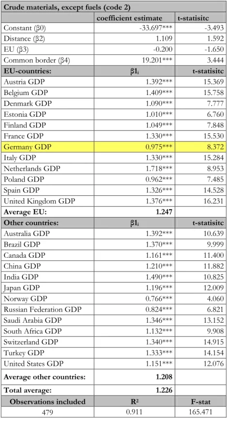
Crude materials except fuels

Table 5.2 shows the regression results for Swedish exports of crude materials except fuels. The dummy variable for EU-membership and the distance variable are insignificant. Thus, it is not possible to draw any conclusions if EU-membership and distance have an effect on Swedish exports of crude materials. Crude material prices are determined on the world market and many of these commodities are even traded on international exchanges. Some are considered investments and are subject to speculations. For example, future contracts and options on crude materials are traded on international commodity exchanges such as the London Metal Exchange (London Metal Exchange, 2012). Moreover, trade contracts within this commodity group often include large quantities when manufacturers purchase materials to ensure efficiency and continuity of production (Abramovitz, 1950).

The coefficient for the common-border-dummy (β4) is very high (19.201) and highly signif-icant. When trading crude materials such as steel, high transportation costs occur due to the great mass of the commodities. Therefore, it is easier and less costly for Swedish firms to transport crude materials just across the border to Norway or to ship them across the Baltic Sea to neighboring countries. Yet, we find that the distance variable is insignificant, which contradicts the argument just given. The negative impact that we expect from in-creasing distance might already be captured by the high positive coefficient for the com-mon-border-dummy and this could have caused an insignificant distance variable coeffi-cient (β2).

The average slope coefficient (β1i) is 1.226. On average the slope coefficient (β1i) for

EU-countries (1.247) is slightly higher than for the other EU-countries (1.208), indicating that Swe-dish exports to EU-countries are more elastic than exports to the other countries. Howev-er, the difference is very small.

The lowest slope coefficient (β1_i) (0.776) and thus the most inelastic are Swedish exports to Norway. Norway imports a lot of crude materials from Russia and Canada (OECD, 2012) and these imports can be substitutes for imports from Sweden.

The largest slope coefficient (β1i) is 1.718 in the case of the Netherlands. This means that

ceteris paribus a one percent increase in the Netherlands’ GDP causes a 1.718 percent in-crease in Swedish exports to the Netherlands. Thus, Swedish exports to the Netherlands are elastic. A reason can be that the Netherlands highly depend on imports of crude mate-rials because they do not have these natural resources in their own country (Ehrlich, 2009). We can even see that the Netherlands are the second largest importer of Swedish crude materials, in 2010 they imported 12 percent of total Swedish exports in this commodity group (see Appendix 4). Moreover, the Netherlands have one of the largest harbors in the world and engage heavily in trade of crude materials. This could explain why Swedish ex-ports of crude materials to the Netherlands are sensitive to changes in GDP.

In 2010 Germany was the country that imported the largest share (15 percent) of total Swedish exports of crude materials, except fuels (see Appendix 4). Germany has a slope coefficient (β1i) of 0.975. Thus, Germany’s demand for Swedish exports of crude materials

is close to unit elastic. Germany’s natural resources are small relative to its large manufac-turing industries. Throughout history Germany has always imported large amounts of crude materials from Sweden. Already during the era of the Hanseatic League, Germany imported iron from Sweden (Heckscher, 1954). Today, Germany also imports great amounts of paper pulp from Sweden for production of paper (Nationalencyklopedin, 2012c). Therefore, it is not surprising to find unit-elastic exports to Germany. Yet, Swedish exports to 25 countries on average are more elastic.

(22)

Table 5.2: Regression results: Exports crude materials, except fuels (dependent) Crude materials, except fuels (code 2)

Constant (β0) -33.697*** -3.493 Distance (β2) 1.109 1.592 EU (β3) -0.200 -1.650 Common border (β4) 19.201*** 3.444 EU-countries: β1i t-statisitc Austria GDP 1.392*** 15.369 Belgium GDP 1.409*** 15.758 Denmark GDP 1.090*** 7.777 Estonia GDP 1.010*** 6.760 Finland GDP 1.049*** 7.848 France GDP 1.330*** 15.530 Germany GDP 0.975*** 8.372 Italy GDP 1.330*** 15.284 Netherlands GDP 1.718*** 8.953 Poland GDP 0.962*** 7.485 Spain GDP 1.326*** 14.528 United Kingdom GDP 1.376*** 16.231 Average EU: 1.247

479 0.911 165.471

(23)

Chemicals

Table 5.3 shows the regression results for Swedish exports for commodity group 5, chemi-cals. We find that the two dummy variables D1_it and D2_i are insignificant. Our model can-not explain if EU membership or a common border have an effect on Swedish exports of chemicals.

As expected, geographical distance has a negative impact on Swedish exports of chemicals: the β2 coefficient is -1.306. This can be due to the fact that some of the goods in this commodity group are difficult and thereby costly to transport because they may be very toxic or explosive. However, this implies that we should have found a significant positive effect from sharing a border which we do not find. A reason can be that statistically the ef-fect of geographical proximity is captured by the negative distance coefficient and that this could have caused the common border dummy to be insignificant.

On average the slope coefficient (β1i) is 1.414, thus a one percent change in foreign GDP

results in a larger than one percent change in exports of chemicals. Swedish exports of chemicals could be elastic because they have gained more importance over the last 20 years. Their share of total Swedish exports has increased from 8.4 percent in 1991 to 12.7 percent in 2009 (see Appendix 3). Another reason could be that chemicals are often used as inter-mediate goods in the production of other investment products. The demand for invest-ment products depends greatly on GDP. Thus, the demand for chemicals highly depends on GDP as well. This is in line with Levchenko et al. (2010) who find that goods that are used as intermediate goods are especially sensitive to changes in demand.

Germany’s slope coefficient (β1i) is 1.262. It is lower than the total average slope coefficient

(β1i) and lower than the EU-countries average slope coefficient (β1i). Hence, Swedish

ex-ports to Germany in this commodity group are relatively less elastic than Swedish exex-ports to the 25 countries on average. Germany’s production of chemical products accounts for 28.8 percent of the total production of chemicals within the EU (Cefic, 2011). Thus, Ger-many does not depend on imports from Sweden to the same extent as other countries do, and for Sweden it could be more difficult to export its products to the German market than to other countries on average.

Another country for which Swedish exports are relatively less elastic than on average are the Netherlands. Their slope coefficient is the lowest among the EU-countries. Here, we see a similar picture as for Germany: 10.2 percent of total production of chemicals in the EU is produced in the Netherlands (Cefic, 2011) and therefore it could as well be difficult for Sweden to export to the Netherlands.

(24)

Table 5.3: Regression results: Exports chemicals (dependent) Chemicals (code 5)

Constant (β0) -2.659 -0.480 Distance (β2) -1.306*** -3.264 EU (β3) 0.060 0.864 Common border (β4) -3.776 -1.179 EU-countries: β1i t-statisitc Austria GDP 1.493*** 28.686 Belgium GDP 1.537*** 29.908 Denmark GDP 1.293*** 16.053 Estonia GDP 1.391*** 16.209 Finland GDP 1.346*** 17.520 France GDP 1.473*** 29.942 Germany GDP 1.262*** 18.852 Italy GDP 1.467*** 29.352 Netherlands GDP 1.152*** 10.447 Poland GDP 1.298*** 17.567 Spain GDP 1.504*** 28.673 United Kingdom GDP 1.466*** 30.103 Average EU: 1.390

479 0.930 214.740

(25)

Manufactured goods

Table 5.4 shows the regression results for Sweden’s export of manufactured goods. Both, the coefficient for the distance variable and the coefficient for the EU-dummy variable are insignificant. However, the coefficient for the common-border-dummy variable is signifi-cant. Sweden exports large amounts of manufactured goods. In 2010, exports in this com-modity group accounted for 18.6 percent of total Swedish exports (see Appendix 3). The coefficient for the border-dummy (β4) is 4.863, thus sharing a border has a positive impact on Swedish exports. Arguably, the negative impact that we expect from geographical dis-tance is captured in this variable.

When looking at the slope coefficients (β1i) it is interesting to see that they are all close to

one. On average the slope coefficient (β1i) is 1.022, the average slope coefficient (β1i) for

EU-countries is slightly higher at 1.057 and the average slope coefficient (β1i) for other

countries slightly lower at 0.992. This means that on average Swedish exports of manufac-tured goods are approximately unit elastic with respect to the trading partner’s GDP. Man-ufactured goods include investment goods and consumer durables. These goods are post-ponable goods since their purchase can often be postponed when the public or personal economy does not allow big purchases. Therefore, the demand for investment goods and consumer durables highly depends on GDP. This is even the case for the demand for im-ports. These results are in line with Baldwin (2009) who stresses the importance of the fact that purchases can be postponed in times of an economic crisis and the implications for both domestic and import demand. The high dependence of demand for durable goods on GDP explains that we do not find inelastic demand.

The slope coefficient (β1i) for Swedish exports of manufactured goods to Germany is

0.988. Even here we see approximately unit elastic Swedish exports. The slope coefficient (β1_i) for Germany is the lowest among all EU-countries, suggesting that even though the differences are very small, Swedish exports of manufactured goods to Germany are the least elastic exports of manufactured goods among the EU-countries. Both countries are known for their high-quality manufactured products and much of their trade in this com-modity group is IIT. Germany has a big manufacturing sector and is a net-exporter of manufactured products (Federal Statistical Office of Germany, 2009). Therefore, it could be relatively more difficult for Sweden to export its manufactured products to the German market than to other EU-countries.

Sweden and Germany have been engaging heavily in trade of manufactured goods since end of the Hanseatic League era (Heckscher, 1954). Over this long period of time reliable relations have been built. We find that German GDP and Swedish exports of manufac-tured goods to Germany go hand in hand: a one percent increase in German GDP results in approximately a one percent increase in Swedish exports to Germany.

Among the trading partners from outside the EU there are some countries that have an even lower slope coefficient (β1i) than Germany. These countries are Canada, China, Japan,

Norway, the Russian Federation and the US. Except for Norway these economies are very large and satisfy their demand for imports by importing from a large pool of countries. Therefore, they have a lot of substitution possibilities for imports from Sweden, leading to inelastic demand for Swedish exports. Moreover, Canada, Japan, Norway and the US have highly developed manufacturing industries on their own that can satisfy domestic demand for manufactured goods.

(26)

Table 5.4: Regression results: Exports manufactured goods (dependent) Manufactured goods (code 6)

Constant (β0) -13.702*** -3.433 Distance (β2) 0.381 1.320 EU (β3) 0.011 0.225 Common border (β4) 4.863** 2.108 EU-countries: β1i t-statisitc Austria GDP 1.059*** 28.255 Belgium GDP 1.069*** 28.892 Denmark GDP 1.071*** 18.456 Estonia GDP 1.092*** 17.670 Finland GDP 1.056*** 19.097 France GDP 1.029*** 29.048 Germany GDP 0.988*** 20.496 Italy GDP 1.034*** 28.736 Netherlands GDP 1.191*** 15.000 Poland GDP 1.002*** 18.846 Spain GDP 1.024*** 27.094 United Kingdom GDP 1.063*** 30.310 Average EU: 1.057