Phase field modeling of flaw-induced hydride precipitation kinetics in metals

(1)

THESIS FOR THE DEGREE OF LICENTIATE OF ENGINEERING

Phase field modeling of flaw-induced hydride precipitation

kinetics in metals

CLAUDIO F. NIGRO

Department of Materials and Manufacturing Technology CHALMERS UNIVERSITY OF TECHNOLOGY

(2)

i

Phase field modeling of flaw-induced hydride precipitation kinetics in metals Claudio F. Nigro

claudio.nigro@mah.se © CLAUDIO NIGRO, 2017.

ISSN 1652-8891 No 113/2017

Department of Materials and Manufacturing Technology Chalmers University of Technology

SE-412 96 Gothenburg Sweden

Telephone + 46 (0)31-772 1000

Chalmers Reproservice Gothenburg, Sweden 2017

(3)

ii

Phase field of flaw-induced hydride precipitation kinetics in metals CLAUDIO NIGRO

Department of Materials and Manufacturing Technology CHALMERS UNIVERSITY OF TECHNOLOGY

Abstract

Hydrogen embrittlement can manifest itself as hydride formation in structures when in contact with hydrogen-rich environments, e.g. in space and nuclear power applications. To supplant experimentation, modeling of such phenomena is beneficial to make life prediction reduce cost and increase the understanding.

In the present work, two different approaches based on phase field theory are employed to study the precipitation kinetics of a second phase in a metal, with a special focus on the application of hydride formation in hexagonal close-packed metals. For both presented models, a single component of the non-conserved order parameter is utilized to represent the microstructural evolution. Throughout the modeling the total free energy of the system is minimized through the time-dependent Ginzburg-Landau equation, which includes a sixth order Landau potential in the first model, whereas one of fourth order is used for the second model. The first model implicitly incorporates the stress field emanating from a sharp crack through the usage of linear elastic fracture mechanics and the governing equation is solved numerically for both isotropic and anisotropic bodies by usage of the finite volume method. The second model is applied to plate geometries containing a notch or not, and it includes an anisotropic expansion of the hydrides that is caused by the hydride precipitation. For this approach, the mechanical and phase transformation aspects are coupled and solved simultaneously for an isotropic material using the finite element method.

Depending on the Landau potential coefficients and the crack-induced hydrostatic stress, for the first model the second-phase is found to form in a confined region around the crack tip or in the whole material depending on the material properties. From the pilot results obtained with the second model, it is shown that the applied stress and considered anisotropic swelling induces hydride formation in preferential directions and it is localized in high stress concentration areas. The results successfully demonstrate the ability of both approaches to model second-phase formation kinetics that is triggered by flaw-induced stresses and their capability to reproduce experimentally observed hydride characteristics such as precipitation location, shape and direction.

Keywords: phase transformation, phase field theory, hydrogen embrittlement, hydride, linear elastic fracture mechanics, finite volume method, finite element method

(4)

(5)

iv

(6)

(7)

vi

The most incomprehensive thing about the world is that it is comprehensible.

- A. Einstein

(8)

vii

Faculty of Technology and Society

(9)

viii

Acknowledgements

This PhD work takes place in the department of Material Science and Applied Mathematics at the Faculty of Technology and Society, Malmö University in cooperation with Material and Manufacturing Technology, Chalmers University of Technology.

I would like to thank my supervisors, Christina Bjerkén and Pär Olsson, for supporting me throughout this project by providing their expertise, knowledge and encouragements. I am also grateful to the whole team of the department of material science and mechanics at Malmö University for welcoming and integrating me with kindness and professionalism. I wish to give a special acknowledgement to my colleague Niklas Ehrlin who shared numerous exciting PhD student activities and interesting discussions.

I wish to thank my collaborators in the project CHICAGO (Crack-induced HydrIde nuCleation And GrOwth) which is a collaboration between the teams of Lund University and Malmö Univeristy. The members, Wureguli Reheman, Martin Fisk, Christina Bjerkén, Per Ståhle, Pär Olsson and I, have allowed carrying out a common project and contributed to the writing of the appended Paper C, which, after finalizations, aims at being published.

Special and obvious thanks are addressed to my wife Pernilla and son Henri, the stars of my life.

This work was funded by Malmö University.

Claudio Nigro Malmö, Sweden March, 2017

(10)

(11)

x

Appended papers

Paper A

Claudio F. Nigro, Christina Bjerkén, Pär A. T. Olsson. Phase structural ordering kinetics of second-phase formation in the vicinity of a crack. Submitted to the International Journal of

Fracture.

A parametric study of a phase-field model for hydride forming kinetics in the vicinity of a sharp crack tip in an isotropic body is performed through the use of a sixth-order Landau potential. The hydride formation is the results of a stress-induced quench of the material in a confined area around the crack or in the whole material depending on the used input parameters.

Paper B

Claudio F. Nigro, Christina Bjerkén, Pär A. T. Olsson. Kinetics of crack-induced hydride formation in hexagonal close-packed materials. Submitted to the Proceedings of the 2016

International Hydrogen Conference. Moran, USA. September 2016.

The model based on the sixth-order Landau potential is applied to two hexagonal close-packed metals: titanium and zirconium. The phase transformation, which occurs in a confined area around the crack tip, displays different shapes, i.e. sizes and symmetries, depending on the considered crack plane whether it is relative to the crystallography, basal or prismatic, and the crack inclination.

Paper C

Wureguli Reheman, Claudio F. Nigro, Martin Fisk and Christina Bjerkén. Phase field model for hydride formation in zirconium alloys. Manuscript form.

A fourth-order Landau potential is used to describe hydride formation including anisotropic swelling of the hydrides. The pilot model is applied to defect-free and notched plates. The numerical method works so that the mechanical and the phase-field equations are solved simultaneously. The results are displayed by the formation of hydrides, which are elongated and grow in preferential directions depending on the principal stress directions. The effect of various material parameters on the phenomenon is studied.

Own contribution

In Paper A and B, the author of this thesis carried out all simulations, numerical implementations and analyzed the results. He also planned the entire work for Paper B. The co-authors participated in writing the manuscripts, discussions and the planning of the work in Paper A. For Paper C, the main author performed all simulations. The author of this thesis took an active part in the planning of the paper, the numerical implementation, the development of the model and manuscript writing.

(12)

(13)

xii

1 Introduction

Hydrogen, the most abundant and lightest chemical element in the universe, has become a major concern for the material industry. Numerous works have shown that it is responsible for degrading the mechanical properties of metals in hydrogen-rich environments, possibly leading to premature fracture. Among hydrogen damage processes stand hardening, embrittlement and internal damage.

Hydrogen embrittlement is generally characterized by the deterioration of the mechanical properties of a material in presence of hydrogen. The phenomenon is well known in aerospace and nuclear industries. In rocket engines being developed for Ariane 6 such as Vinci and Vulcain 2, hydrogen is thought to be utilized as fuel and cooler and therefore interacts with some engine components. The properties of nickel superalloys, traditionally used in high-temperature areas such as the combustion chamber (Kirner, et al., 1993) and the nozzle, have been observed to be derogated in presence of hydrogen (Fritzemeier & Chandler, 1989). Brittle compounds, titanium hydrides, are likely to form in colder engine parts made of titanium alloys when in contact with hydrogen and can embrittle the structure. In nuclear reactor pressure vessels, atomic hydrogen (H) penetrates zirconium-based cladding and pressure tubes where potentially forms brittle zirconium hydrides (Puls, 2012). Hydride formation, a second-phase precipitation, is one stage of the complex mechanism of delayed hydride cracking (DHC) (Northwood & Kosasih, 1983; Coleman, 2003), which is one of the most notorious mechanisms of hydrogen embrittlement in nuclear industry. It can be enhanced by the presence of material defects, which acts as stress concentrators and hydrogen trapping sites.

Knowledge of hydride formation kinetics is fundamental in order to predict the life time of a metallic structure subjected to DHC in a hydrogen-rich environment. For this purpose, modeling is found to be an economically beneficial route to develop knowledge in the field. Thus, in this context, the present study focuses on modeling a second-phase formation in the presence of a crack and notch.

The second-phase formation has been modeled over the years through the use of different approaches such as the sharp-interface and phase field methods (PFM). In the present work, two different models based on phase field theory (PFT) are developed to model second phase formation, especially in the vicinity of stress concentrators. Linear elastic fracture mechanics (LEFM) is adopted in the first presented model in order to account for the stress field in presence of a sharp crack. The problem is solved with finite volume method and the model formulation allows both first- and second-order transformations to occur. In the second model that is still a pilot model the anisotropic material swelling caused by zirconium hydride formation is explicitly taken into account while only first-order transformations are allowed. The second model is applied to a defect-free plate and a notched plate, which are subjected to external tensile stress. The numerical scheme employs the finite element method to concurrently solve the mechanical and phase-field governing equations, which are strongly coupled.

(16)

Hydrogen degradation

2

2 Hydrogen degradation

Hydrogen is known for its capacity to alter the properties of metals such as steels, aluminum (Al), titanium (Ti), zirconium (Zr), nickel (Ni) and their respective alloys. In hydrogen rich environments, failures can arise from residual and/or applied tensile stresses combined with hydrogen-metal interactions. Loss of ductility and reduction of load-carrying capacity are often observed in a metal because of such interaction, e.g. in steels, nickel-base alloys, aluminum alloys, and titanium. Such deteriorations of materials are usually referred to as hydrogen embrittlement. For example, hydrogen environment embrittlement characterizes the situations where materials undergo plastic deformation while in contact with hydrogen-rich gases or corrosion reactions. Molecular hydrogen undergoes adsorption at the metal free surface, which weakens the H-H bond and promotes its dissociation into atomic hydrogen within the metal lattice (Christmann, 1988; Hicks & Altstetter, 1992). Several other types of hydrogen damage are known as hydrogen attack, blistering and hydride formation (Cramer & Covino, 2003). Formation of gas or non-metallic compounds emanates from these hydrogen degradation processes. Hydrogen attack affects carbon and low-alloyed steels and usually occurs at high temperature. The inner hydrogen reacts with carbon to form methane within the material. Possible damaging consequences are crack formation and decarburization. Blistering is the result of plastic deformation induced by the pressure of molecular hydrogen that is formed near internal defects. The gas formation occurs due to the diffusion of atomic hydrogen to these regions. Once formed, blisters are often observed to be fractured.

During service and in presence of hydrogen, the formation of non-metallic compounds, the so-called hydrides, can be responsible for material embrittlement (Puls, 2012; Northwood & Kosasih, 1983; Coleman & Hardie, 1966). A well-known associated fracture mechanism example is the so-called delayed hydride cracking (DHC). It is a form of localized hydride-embrittlement that is characterized by a combination of processes, which involve hydrogen diffusion, hydride precipitation including subsequent hydride expansion – the phase transformation induces a swelling of the reacting zone – and possible crack growth (Coleman, 2003). Driven by the stress, hydrogen migrates towards the region of high tensile stress concentration, e.g. in the vicinity of defects or in residual stress regions, leading to supersaturation. Brittle hydrides form once the solid solubility limit is exceeded and usually develop orthogonally to the tensile stress until a critical size is reached. Thereafter, the localized hydrided region can be fractured under the present stress. The possible resulting crack is then likely to propagate through the material by the same described mechanism in a stepwise manner (Puls, 2012). The adjective “delayed” reflects the fact that it takes time for hydrogen to diffuse towards the crack tip and react with the matrix to form a hydride. (Banerjee & Mukhopadhyay, 2007). For instance, DHC was observed to operate in Zr-2.5Nb alloy pressure tubes in nuclear industry (Singh, et al., 2004).

A number of materials such as zirconium, titanium, hafnium, vanadium and niobium have a low solubility of hydrogen, and, therefore, can form different types of hydride phases depending on e.g. hydrogen concentration and temperature history (Coleman, 2003). For example, Figure 1 shows the phase diagram for the Zr-H system, which constitutes five solid phases (Zuzek, et al., 1990). The solid solution phase , with a hexagonal close-packed

(17)

Hydrogen degradation

3

(HCP) crystal structure, has a low solubility of hydrogen, while the high-temperature allotrope -Zr (BCC) has a high solubility. Two stable hydride phases are identified, the FCC - and FCT -phases, respectively. The -phase is considered metastable and has FCT structure (Barrow, et al., 2013). Additionally, a crystal structure denoted  has recently been observed and may be a possible precursor to the formation of - and -phases (Zhao, et al., 2008). The phase diagram of the Ti-H system is very similar to that of Zr-H, and only the exact location of the phase boundaries differs.

Figure 1: Phase diagram for the Zr-H system, reproduced with permission from (Maimaitiyili, et al., 2015).

The hydride precipitates generally appear as needles or platelets in the solid solution -phase of Zr and Ti alloys, and the formation may occur either in grains or grain boundaries in polycrystals (Beck & Mueller, 1968; Coleman, 2003). A preferred hydride orientation may exist and is affected by the crystal structure and texture emanating from the manufacturing process and the possible presence of applied and residual stresses (Chu, et al., 2008; Northwood & Kosasih, 1983). Some hydrides such as andhydrides in zirconium-based alloys have been observed to exhibit a volume change when they form (Barrow, et al., 2013). For instance, the global swelling of the unconstrained andhydrides, which results from anisotropic dilatational misfits, has been theoretically estimated to be between 10% and 20% with respect to untransformed zirconium, (Carpenter, 1973). The hydrides are more brittle than the -phase, and the fracture toughness of a hydride can be orders of magnitude lower than the solid solution. For example, the fracture toughness KIC of pure -Ti at room

temperature is around 60 MPa ∙ m1 2⁄ _{(Welsch, et al., 1994) while for titanium-based}

(18)

Linear elastic fracture mechanics

4

fracture toughness was measured to be around 70 MPa ∙ m1 2⁄ _{with quasi-zero hydrogen}

content, while that of the δ-hydride (ZrHx, x =1.5−1.64) is found to be approximately

1 MPa ∙ m1 2⁄ _{at room temperature (Simpson & Cann, 1979). In addition, as the hydrogen}

content increases global KIC of hydrided metals may decrease. For the Zr-2.5Nb alloy with a

hydrogen-zirconium ratio of 0.4, the fracture toughness is found between 10 and 15 MPa ∙ m1 2⁄ _{(Simpson & Cann, 1979). Of great concern is that the brittle hydrides are}

observed to form in high stress concentration regions such as in the vicinity of notches, cracks and dislocations, where stress gradient drives hydrogen diffusion until the material exceeds its solubility limit inducing precipitation (Takano & Suzuki, 1974; Birnbaum, 1976; Grossbeck & Birnbaum, 1977; Cann & Sexton, 1980; Shih, et al., 1988; Maxelon, et al., 2001). Under stress and deformation of the metal, and owing to their low fracture toughness, hydrides can be fractured along their length, e.g. in Ti (Shih, et al., 1988; Xiao, et al., 1987), in Zr: (Cann & Sexton, 1980; Östberg, 1968), in Hf (Seelinger & Stoloff, 1971); in V: (Takano & Suzuki, 1974; Koike & Suzuki, 1981); and in Nb: (Matsui, et al., 1987), or across their thickness, e.g. in Ti: (Beevers, et al., 1968) and in Zr: (Coleman & Hardie, 1966; Westlake, 1963).

3 Linear elastic fracture mechanics

A number of models about failure mechanisms were published in the 20th century (Inglis, 1913; Griffith, 1920; Westergaard, 1939; Irwin, 1949; Orowan, 1949; Irwin, 1956), some of which were used by Irwin to develop a description of the stresses and displacements ahead of a crack using a single parameter, the so-called stress intensity factor, which is connected to the energy release rate, the external stress, the crack length and the geometry of the considered structure (Irwin, 1957). This stress and displacement analysis is still used in fracture mechanics for bodies displaying small plastic zones around crack tips. This theory is called linear elastic fracture mechanics (LEFM).

The fracture operates in three different basic modes depicted in Figure 2. Mode I, also called the tensile opening mode, occurs when the crack walls separate symmetrically with respect to the crack axis and in the crack-plane normal direction. In mode II, the in-plane sliding mode, the crack surfaces are sheared from one another and the sliding is achieved parallel to the plane of the crack and perpendicular to the crack front. Mode III is also known as the tearing or anti-plane shear mode. In this situation, the crack surfaces slide relative to each other in opposite directions parallel to the crack front and the crack plane.

(19)

5

Figure 2: Illustration of the three fracture modes.

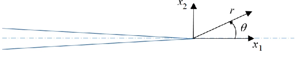
By considering fracture problems in a polar coordinate system as presented in Figure 3 within LEFM, the stress intensity factor gives the expressions of the components of the stress tensor in the vicinity of the crack-tip for a specific mode of fracture in a linear elastic medium, as expressed in (Anderson, 2005) as 𝜎𝑖𝑗 = 𝐾 √2𝜋𝑟𝑓𝑖𝑗(𝜃) + ∑ 𝐵𝑚𝑟 𝑚 2_𝑔_𝑖𝑗(𝑚)_(𝜃) ∞ 𝑚=0 , (1)

where 𝑟 is the distance from the origin that is the crack-tip, 𝐾 is the stress intensity factor for the considered mode, 𝑓_𝑖𝑗 is a trigonometric and dimensionless function, 𝑔_𝑖𝑗(𝑚) and 𝐵_𝑚 designates a trigonometric function for the 𝑚𝑡ℎ_{term and its amplitude. The indices 𝑖 and 𝑗 are}

taken in {1,2,3}. The high-order terms become negligible as 𝑟 is small. Therefore, in the close region of the crack-tip, the stress approximately varies in 1/√𝑟.

Figure 3: Illustration of the two-dimensional stress in different coordinate systems and bases in the vicinity of a crack tip.

(20)

6

Although the polar coordinates are used to express the stress components around the crack tip the stress components can be written in the Cartesian base as well as in the polar base as illustrated in Figure 3.

For a linear elastic medium, the strain tensor 𝜀𝑖𝑗 is related to the stress tensor through the use

of Hooke’s law as,

𝜀_𝑖𝑗 = 𝑠_{𝑖𝑗𝑘𝑙} 𝜎_𝑘𝑙, (2)

where 𝑠_{𝑖𝑗𝑘𝑙} is the compliance tensor, and is also connected to the displacement field 𝑢_𝑖 through 𝜀_𝑖𝑗 =1 2( 𝜕𝑢𝑖 𝜕𝑥_𝑗 + 𝜕𝑢_𝑗 𝜕𝑥_𝑖). (3)

In planar fracture analysis, the out-of-plane stress and strain contributions can be different from zero depending on the assumed plane-state condition. The latter presents two distinct variants: plane strain and plane stress. In plane stress condition, the stress components relative to the out-of-plane direction are zero. In contrast, in plane strain, the strain components relative to the out-of-plane direction are zero. A plane strain condition is suitable for a planar study of a thick body and the plane stress condition is applicable to thin bodies. In a Cartesian base (𝑥₁, 𝑥₂), in fracture mode I and for plane-strain conditions, the stress components lying in the close region of a crack tip in an isotropic and linear elastic body are expressed as in (Anderson, 2005) as Eq.(1) with

𝑓11(𝜃) = cos 𝜃 2[1 − sin 𝜃 2sin 3𝜃 2 ], (4) 𝑓₂₂(𝜃) = cos𝜃₂[1 + sin𝜃 2sin 3𝜃 2], (5) 𝑓12(𝜃) = sin 𝜃 2cos 𝜃 2cos 3𝜃 2, (6)

and 𝜎₃₃= 𝜈(𝜎₁₁+ 𝜎₂₂), where 𝜈 is the Poisson’s ratio. The associated displacement field for such body is given as

𝑢1 = 2 𝐾_𝐼 (1 + 𝜈) 𝐸 √ 𝑟 2𝜋cos 𝜃 2[1 − 2𝜈 + sin2 𝜃 2], (7) 𝑢2 = 2 𝐾_𝐼 (1 + 𝜈) 𝐸 √ 𝑟 2𝜋sin 𝜃 2[2 − 2𝜈 + cos2 𝜃 2], (8)

(21)

Phase field theory for microstructure evolution

7

Paris and Sih (Paris & Sih, 1965) developed a description of the anisotropic linear-elastic crack-tip stress fields. In a Cartesian base (𝑥₁, 𝑥₂), and in fracture mode I, it is expressed as in Eq.(1) with 𝑓₁₁(𝜃) = Re { 𝜇1𝜇2 𝜇₁− 𝜇₂( 𝜇₂ √cos 𝜃 + 𝜇2sin𝜃 − 𝜇1 √cos 𝜃 + 𝜇1sin𝜃 )} , (9) 𝑓22(𝜃) = Re { 1 𝜇1 − 𝜇2( 𝜇₁ √cos 𝜃 + 𝜇2sin𝜃 − 𝜇2 √cos 𝜃 + 𝜇1sin𝜃 )} , (10) 𝑓₁₂(𝜃) = Re { 𝜇1𝜇2 𝜇₁− 𝜇₂( 1 √cos 𝜃 + 𝜇1sin𝜃 − 1 √cos 𝜃 + 𝜇2sin𝜃 )}, (11)

with μ₁ and μ₂ being the conjugate pairs of roots of

𝑆₁₁ 𝜇4_{− 2𝑆}

16 𝜇3+ (2𝑆12+ 𝑆66) 𝜇2− 2𝑆26𝜇 + 𝑆22= 0. When μ1= μ2 , the stress field

relations are reduced to the isotropic ones (Paris & Sih, 1965). The coefficients 𝑆_𝑖𝑗 are the components of the compliance matrix in plane stress or in plane strain conditions in a determined crystal plane, such that,

[ 𝜀₁₁ 𝜀22 2𝜀12 ] = [ 𝑆11 𝑆12 𝑆16 𝑆₁₂ 𝑆₂₂ 𝑆₂₆ 𝑆₆₁ 𝑆₆₂ 𝑆₆₆] [ 𝜎₁₁ 𝜎22 𝜎12 ]. (12)

The planar compliance components 𝑆_𝑖𝑗 are, therefore, combinations of the three-dimensional compliance components 𝑠_{𝑖𝑗𝑘𝑙}. The displacements of the anisotropic linear-elastic crack-tip area can successively be deduced by using Eqs.(9)-(12).

4 Phase field theory for microstructure evolution

Material processing, including solidification, solid-state precipitation and thermo-mechanical processes, is the origin of the development of material microstructures. The latter generally consists of assemblies of grains or domains, which vary in chemical composition, orientation and structure. Characteristics of the microstructure such as shape, size and distribution of grains, impurities, precipitates, pores and other defects have a strong impact on the physical properties (e.g. thermal and electrical conductivity) and mechanical performance of materials. Therefore, the study of mechanisms causing microstructural changes appears necessary to predict the modifications of material properties and, thus, take action to avoid associated malfunctioning components or failure of structures.

Conventionally, the physical and thermodynamic mechanisms acting in an evolving microstructure such as heat diffusion and impurity transportation are modeled through the use of a time-dependent partial differential equations and associated boundary conditions. This is, for instance, the case in sharp-interface approaches, where the interfaces between the different microstructure areas are supposed sharp as presented in Figure 4a and their positions need to be explicitly followed with time. However, some phenomena are not suitable for

(22)

sharp-Phase field theory for microstructure evolution

8

interface modeling when they are combined with other effects (Haataja, et al., 2005). In addition, complex morphologies of grains are hard to represent mathematically by the sharp-interface approaches when the sharp-interfaces interact with each other during phase transformation, e.g. interface merging and pinch-off within coalescence and splitting of precipitates. Moreover, such modeling is found to be more computationally demanding than diffuse-interface approaches. Therefore, sharp diffuse-interface models are often more appropriate for one-dimensional problems or simple microstructural topologies (Provatas & Elder, 2010; Moelans, et al., 2008).

(a) (b)

Figure 4: Illustration of (a) a sharp interface and (b) a smooth interface.

An alternate way to describe the microstructure evolution is to use phase field methods (PFM), which also employ kinetics equation. This type of modeling provides a continuous and relatively smooth description of the interfaces as illustrated in Figure 4b. The microstructure is represented by variables, also called phase-field variables, which are continuous through the interfaces and are functions of time and space. Thus, unlike sharp interface models, the position of the interface is implicit and determined by the variation of the variable value. Moreover, no boundary conditions are necessary inside the whole system except at the system boundary. Initial conditions are, however, still required. Consequently, PFT allows not only the description of the evolution of simple but also complex microstructural topologies unlike sharp-interface problems. For instance, the dendritic solidification with its complex features was successfully modeled through the use of PFM (Kobayashi, 1993; Kobayashi, 1994).

From the second part of the 20th century to nowadays, phase-field modeling has found a lots of applications in material science processes such as solidification, solid-state phase transformation, coarsening and grain growth, crack propagation, dislocation dynamics, electro migration, solid-state sintering and processes related to thin films and fluids. A number of these achievements is compiled in (Moelans, et al., 2008; Chen, 2002; Steinbach, 2009; Shen & Wang, 2009). More recent publications show that PFM is a current research field when it comes to modeling phenomena which involve some of the mechanisms listed in this paragraph (Bair, et al., 2017; Chang, et al., 2016; Hektor, et al., 2016; Kiendl, et al., 2016;

(23)

9

Schneider, et al., 2016; Shanthraj, et al., 2016; Stewart & Spearot, 2016; Sulman, 2016; Tourret, et al., 2017; Wu & Lorenzis, 2016).

4.1 The phase-field variables

In PFT, a microstructural system is described through the use of single or multiple phase-field variables. Depending on the type of quantity it is connected to, a field variable can be conserved or non-conserved. Conserved variables customary refer to local composition quantities such as the concentration of chemical species. They can also be associated with density and molar volume (Shen & Wang, 2009). According to Moelans, the non-conserved phase-field variable category contains two groups of variables, which are utilized to distinguish two concurrently prevailing phases: the phase-field and the order parameters (Moelans, et al., 2008). The former are phenomenological parameters indicating the presence of a phase in a specific position and the latter designate the degree of symmetry of phases, giving information about the local crystal structure and orientation. However, this distinction is often not made. Thus, conserved and non-conserved phase-field variables can often be found to be respectively termed conserved and non-conserved order parameters (Shen & Wang, 2009; Jokisaari, 2016; Provatas & Elder, 2010). This paper uses these latter denominations.

In the theory suggested by Landau, a bi-phase system may be defined by the presence of an ordered phase and a disordered phase depending on their degree of symmetry. The coexisting phases are associated with specific values of the non-conserved order parameter 𝜙 or other conditions on the phase variable, e.g., traditionally, 𝜙 = 0 for the disordered phase and 𝜙 ≠ 0 for the ordered phase (Landau & Lifshitz, 1980). Depending on the formulation, the phase-variable can be defined with different values in order to account for the phases of a system from model to model. It can be found that a disordered phase corresponds to 𝜙 = 0 and the ordered phase associated with 𝜙 = −1 or 1 (Moelans, et al., 2008). In (Ståhle & Hansen, 2015), 𝜙 = −1 accounts for an empty space and 𝜙 = +1 denotes a filled space. A one-dimensional example of the variation of the order parameter through an interface is illustrated in Figure 4b. The significance and interpretation of a conserved phase field variable is analogue to those of the non-conserved order parameter. Thus, different values of the chemical concentration can be used to distinguished different microstructural domains for example.

The conserved order parameter is usually a scalar but the non-conserved variable can be employed as a vector. When used as a scalar, it can be considered a spatial average of its vector form (Provatas & Elder, 2010). The components of the non-conserved order parameter vector are also responsible for the orientation of the phases (Wang, et al., 1998; Bair, et al., 2016).

(24)

10

4.2 Minimization of the free energy of a system

4.2.1 The total free energy

In nature, systems strive to find equilibrium by minimizing its energy. In phase-field theory, the evolution of a microstructure, e.g. a phase transformation, is governed by a kinetics equation based on the minimization of the total free energy F. The latter can be expressed as the sum of characteristic free energies which are functions of time, space, pressure, temperature and the phase-field variables. The total energy boils down to

F=F_{𝑏𝑢𝑙𝑘}+F_{𝑔𝑟𝑎𝑑}+F_𝑒𝑙+ ⋯, (13)

where the bulk or chemical free energy F_{𝑏𝑢𝑙𝑘} is the Landau free energy functional. In Paper C the chemical free energy is denoted F_𝑐ℎ. The gradient energy F_{𝑔𝑟𝑎𝑑} accounts for the presence of interfaces through a Laplacian term and is connected to the interfacial energy. The bulk energy and gradient energy can be regrouped in a single term, the structural free energy F_𝑠𝑡𝑟 (Massih, 2011), as in Paper A and B. The elastic-strain free energy F_𝑒𝑙 represents the energy stored by a system subjected to stresses or undergoing deformation. The energy associated with a microstructural swelling or dilatation due to phase transformation can be included in the elastic-strain energy term, e.g. in Paper C, where the elastic-strain energy is denoted F_𝑠𝑡, or appear in the equation as an independent term, the interaction energy denoted F_𝑖𝑛𝑡, e.g. in Paper A and B and (Massih, 2011). Finally, other free energy terms can be added to the expression such as free energies related to electrostatics and magnetism.

4.2.2 The Landau potential and system equilibrium

The Landau free energy density is a thermodynamic potential, which can be used to characterize the thermodynamic state of the system near a phase transition. The Landau potential can be written in terms of pressure 𝑃, temperature 𝑇 and an order parameter 𝜙. It was suggested by Landau that it can be formulated as a polynomial expansion in power of 𝜙 (Landau & Lifshitz, 1980) as

ψ_{𝑏𝑢𝑙𝑘}(𝑃, 𝑇, 𝜙) =ψ_{𝑏𝑢𝑙𝑘}(𝑃, 𝑇, 𝜙 = 0) + ∑𝐵𝑛(𝑃, 𝑇) 𝑛

𝑁 𝑛=1

𝜙𝑛_, ₍₁₄₎

where 𝐵_𝑛 denotes the coefficient of the phase-field variable, and can be a function of pressure and temperature. In this paper, the pressure 𝑃 is assumed constant in all descriptions. Landau’s theory supposed that 𝐵2 = 𝑎0(𝑇 − 𝑇𝑐) where 𝑎0 is a phenomenological positive

constant, 𝑇 is the material temperature and 𝑇_𝑐 is the phase transition temperature. The Landau free energy can be chosen symmetric, for instance, in case of a simple bi-phase system for driven by a symmetric phase diagram, but can also be non-symmetric, for example, in case of a gas-liquid transition or system with a phase diagram including a critical point (Provatas & Elder, 2010).

(25)

11

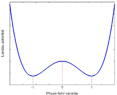
A typical example of one form of the symmetric forth-order potential, where 𝐵₁ = 𝐵₃ = 0, 𝐵2 ≠ 0 and 𝐵4 > 0, representing the thermodynamic potential of a binary system is presented

in Figure 5. In this specific case, the Landau potential curve displays a characteristic shape called double well. The thermodynamic potential finds minima for 𝜙 = −1 and 1 and a maximum for 𝜙 = 0.

Figure 5 : Example of a Landau potential profile.

More generally, the zero root of a symmetric forth-order potential with 𝐵₄ > 0 can be defined to correspond to a solid solution and the non-zero roots represent the second phase. In the absence of other energy contributions, the prevailing phase is the one for which the order parameter values minimizes the Landau potential. Therefore, in the considered system location where the Landau expansion appearance is similar to that in Figure 5, the second phase should develop and dominate the solid solution. The described situation may be characterized by 𝑇 < 𝑇𝑐, i.e. 𝐵2 < 0 and result, for example, from a phase transformation

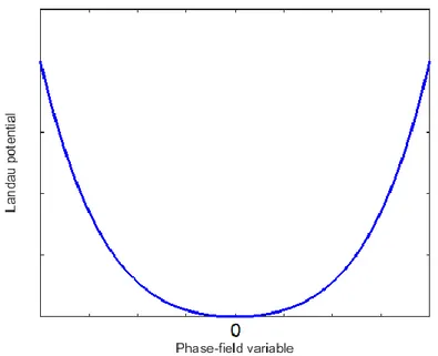
caused by an undercooling of a pure solid solution. The Landau potential appearance for 𝑇 > 𝑇𝑐, i.e. 𝐵2 > 0 is depicted in Figure 6. In this situation, there is only one minimum and it

is associated with 𝜙 = 0. This indicates the prevalence of the solid solution with respect to the second phase. Consequently, a temperature variation can modify the shape of the curve.

(26)

12

Figure 6 : Example of a Landau potential profile with 𝑇 > 𝑇𝑐.

When the temperature is constant a phase transformation can be triggered by the presence of energy contributions, such as those presented in the section 4.2.1, which are different from F_{𝑏𝑢𝑙𝑘}. For instance, in (Bjerkén & Massih, 2014), the elastic strain energy, which is added to the bulk energy, has an active role in the phase evolution. The transition temperature varies depending on the gradient of stress and strain induced by a dislocation. Thus, the total free energy density profile changes with distance from the flaw. This can result in the formation of a second phase where 𝑇 < 𝑇_𝑐 in the vicinity of the dislocation, while the rest of the material is in a state of solid solution (𝑇 > 𝑇𝑐).

In other phase field models where a symmetric fourth order Landau expansion is employed, some of the energy terms other than the bulk energy one are formulated so that they contribute to a breaking of the symmetry of the system total free energy density. For example, in (Ståhle & Hansen, 2015), the elastic strain energy includes first and third order terms in 𝜙 and modifies the double well shape. An illustrated example of such change is given in Figure 7. In such situation displayed at specific position and instant, the solid solution and the second phase are represented by 𝜙 = −1 and 𝜙 = 1 respectively. In Figure 7, the non-symmetric terms promote the domination of the second phase. In this formulation, if the total free energy density profile was similar to the Landau potential’s one presented in Figure 5 it would represent a microstructure where both phases can coexist.

(27)

13

Figure 7 : Example of a total free energy profile for which the elastic strain energy induced a

appearance.

Two types of phase transitions exist: first and second order transformation. First order transitions are characterized by a discontinuous derivative of the system free energy with respect to a thermodynamic variable and a release of latent energy. Nucleation of a metastable state of the matter is the starting point of a first-order transformation. In addition, some materials, which undergo such type of transformation, are able to display the coexistence of different phases for many thermodynamic conditions and compositions. Transformation examples such as liquid solidification and vapor condensation are part of the first order transition category. For the second order transition the system free energy first derivative is continuous with no release of latent heat. Nevertheless, the second derivative of the system free energy of the system is discontinuous. In this case, the transformation is triggered by the presence of thermal fluctuations. This category includes phenomena such as phase separation of binary solutions, spinodal decomposition in metal alloys or, below Curie temperature, spontaneous ferromagnetic magnetization of iron (Provatas & Elder, 2010).

A relation exists between the order of the transformation and the formulation of the free energy of the system. In the literature, the formulations using a fourth-order Landau expansion for the bulk energy can mainly display first and second order transformation (Cowley, 1980). A symmetric fourth-order Landau potential usually represents second-order phase transformation when 𝐵4 > 0. First-order transition are mostly modeled through the use

of an asymmetric double well potential but can also be described by a symmetric fourth-order polynomial with 𝐵₄ < 0. However, in the latter case, since the fourth order Landau potential is unbounded, it is unpractical to use. In order to use a symmetric Landau expansion to represent first-order transition, higher order terms are required.

(28)

14

As energies other than the bulk free energy are included in the total free energy of the system, first- and second-order transformations may occur depending on the formulation of the extra terms. For example, in the first type of models presented above, where the transformation is driven by a stress-induced change of the phase transition temperature and 𝐵4 > 0, the

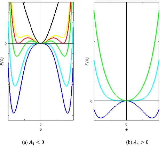
elastic-strain energy only affects the quadratic term of the double-well potential. Consequently, the symmetry of the system free energy is conserved and the transformation is of second order. In the second presented type of formulations illustrated in Figure 7, first-order transitions are considered since non-symmetric terms such as first- and third-order terms in 𝜙 are added by the elastic-strain energy to the total free energy of the system. Further, more complex forms of the free energy density of the system allow representing both order transformations as in (Bjerkén & Massih, 2014), where the Landau expansion includes higher order terms of the order parameter. A model using a symmetric sixth order polynomial for the system free energy density is illustrated in Figure 8.

(a) 𝐴4 < 0 (b) 𝐴4 > 0

Figure 8 : Free energy of a system versus phase field variable obtained with a model where the bulk energy is represented by a 6th order Landau expansion.

In this example, stability of the system is ensured by setting 𝐵₆ > 0. The sign and value of the coefficients 𝐵2 and 𝐵4 affect the appearance of the free energy. Figure 8a and Figure 8b

respectively present the free energy density polynomial for 𝐵₄ < 0 and 𝐵₄ > 0. The zero value of the phase field variable corresponds to the prevalence of solid solution (𝑇 > 𝑇_𝑐 or 𝐵₂ > 0) while non-zero values designate the second phase domination (𝑇 < 𝑇_𝑐 or 𝐵₂ < 0). In

(29)

15

both figures, the transition from upper to lower curves represents an increase in the material transition temperature. In the situation depicted in Figure 8a, where metastable phases marked by local minima (green and yellow curves) possibly exist, first-order transformations may occur whereas in the case illustrated in Figure 8b only second-order transitions may take place. Note that for 𝐵₄ < 0, the phases may coexist. This situation is represented by the red curve in Figure 8a.

In an evolving microstructure, the total free energy profiles changes with time and location. This evolution is governed by the kinetic equations.

4.2.3 The kinetic equations

As mentioned in section 4.2.1, the kinetic equations govern the evolution of the microstructure. Employed to model the variation of the phase-field variables in time and space, the governing equations are introduced as the Cahn-Hilliard equation (Cahn, 1961) and the time-dependent Ginzburg-Landau (TDGL) equation. The latter is also named the Allen-Cahn equation (Allen & Allen-Cahn, 1979). The Allen-Cahn-Hilliard and the TDGL equations respectively use a conserved and a non-conserved order parameter. In both equations, the minimization of the total free energy is obtained through the use of a functional derivative. For a quasi-static transformation, the system is in equilibrium or its free energy reaches a minimum when the functional derivative is zero. For a dynamic evolution of the microstructure, the relaxation toward equilibrium is controlled by a partial derivative of the phase-field variable with time and a positive kinetic coefficient (Gurtin, 1996). The latter is termed mobility and is denoted by 𝐿 in the TDGL. The kinetic coefficient is the diffusion coefficient 𝐷 in the Cahn-Hilliard equation. For a scalar order parameter 𝜂 and without thermal fluctuations, the Allen-Cahn equation can be written as in

𝜕𝜂 𝜕𝑡= − L

δF

𝛿𝜂. (15)

The Cahn Hilliard equation is derived from a mass balance as in (Gurtin, 1996) and, for a conserved order parameter 𝜓 and without thermal fluctuations, it is expressed as

𝜕𝜓

𝜕𝑡 =∇2(D δF

𝛿𝜓). (16)

The use of phase-field theory and linear elastic fracture mechanics respectively described in sections 3 and 4 are used to build up two models, which are presented in the in the next sections of this paper.

(30)

Phase-field models for second-phase formation in presence of a crack

16

5 Phase-field models for second-phase formation in

presence of a crack

5.1 Introduction and motivation

Over the years, models have been developed to predict and simulate second phase nucleation and formation in materials (Varias & Massih, 2002; Jernkvist & Massih, 2014; Bair, et al., 2016; Massih, 2011; Bjerkén & Massih, 2014; Ma, et al., 2006; Deschamps & Bréchet, 1998; Gómez-Ramírez & Pound, 1973; Thuinet, et al., 2012; Shi & Xiao, 2015), some of which are based on PFT and have found applications in hydride formation modeling within HE (Bair, et al., 2016; Massih, 2011; Ma, et al., 2006; Thuinet, et al., 2012; Shi & Xiao, 2015). Moreover, PFT has lately been used increasingly for phase precipitation modeling. This is probably due to its practicality for modeling complex microstructure topologies and smooth interfaces. Depending on the extra energy terms and a considered fourth-order Landau potential form, the formulation of the total energy is either symmetric or asymmetric. Therefore, models based on fourth-order Landau potential cannot suitably represent both types of phase transitions unlike higher order polynomials. A sixth order Landau potential based model has been presented in (Massih, 2011; Massih, 2011; Bjerkén & Massih, 2014) and applied to crack- and dislocation-induced hydride formation although no kinetic study was carried out in case of cracks with this model. In addition, regarding pure phase transition, the conserved and non-conserved phase field variables can be found to be coupled and, therefore, the Cahn-Hilliard and the TDGL equations can be solved simultaneously (Bair, et al., 2016). The mechanical aspect of the transformation is usually treated as uncoupled from that of the phase field. However, since hydride precipitation induces a material swelling and, therefore stresses and strains, it can be thought that a strong coupling exists between phase transformation and the mechanical behavior of the material. It seems therefore necessary to solve the mechanical and phase-field equations simultaneously to ensure a coupling and a stable solution scheme. In this thesis, PFT is chosen to model hydride formation with two different approaches. The first one is based on Massih and Bjerken’s work (Massih, 2011; Bjerkén & Massih, 2014) where a scalar structural order parameter is employed to describe the crack-induced second phase precipitation for different sets of Landau potential coefficients. Both order transitions can be represented with this model. The mechanical aspect is implicitly incorporated in the mathematical formulation through the use of LEFM relations for isotropic and anisotropic materials. The second approach proposes to use a fourth-order double-well expansion for a structural order parameter scalar to account for hydride formation. In this second model, the mechanical and phase transformation aspects are fully coupled. Both presented models allow describing the kinetics of the second-phase precipitation thanks to the use of the TDGL.

(31)

17

5.2 Description of the models

5.2.1 Model 1

In this model, the spatial position of a particle can indifferently be referred through a Cartesian or a polar coordinate system. Thus, the position vector 𝑥_𝑖 is respectively defined by

(𝑥₁, 𝑥₂, 𝑥₃) or (𝑟, 𝜃, 𝑧), and the origin is defined at the tip of a mode-I crack as presented in Figure 9.

Figure 9: Geometry of the system.

The non-conserved order parameter scalar 𝜂 is chosen to describe the evolution of the microstructure such that 𝜂 = 0 designates the matrix or the solid solution and 𝜂 ≠ 0 represents for the second phase. The order parameter may be thought as the probability of phase transformation. Moreover, the diffusional aspect, usually described by a conserved order parameter, is ignored. Therefore, the phase transformations considered in this model may be seen as diffusionless.

The total free energy density of the system with a volume 𝑉 is derived from Eq. (13) and becomes:

F = ∫ [𝑔₂(∇𝜂)2_{+ 𝜓(𝜂) +}1

2𝜎𝑖𝑗𝜀𝑖𝑗𝑒𝑙− 𝜉 𝜂2𝜀𝑙𝑙] 𝑑𝑉, (17) where the sum of the first two terms on the right hand side is equal to the structural free energy F_𝑠𝑡𝑟, the third term is the elastic-strain energy and the last term represents the interaction energy F_𝑖𝑛𝑡. The coefficient 𝑔 is positive, and is related to the interfacial energy and the interface thickness. The phase transformation-induced dilatation of the system and lattice misfit are represented by F_𝑖𝑛𝑡 and include a positive constant 𝜉, called striction factor in (Massih, 2011). The tensor quantities 𝜎_𝑖𝑗, 𝜀_𝑖𝑗 and 𝑢_𝑖 respectively accounts for the stress tensor, the strain tensor and the displacement field. The sixth order Landau potential 𝜓 is expressed as 𝜓(𝜂) = 1 2𝛼0𝜂2+ 1 4𝛽0𝜂4+ 1 6𝛾𝜂6, (18)

where 𝛼₀, 𝛽₀ and 𝛾 are constants related to temperature and the stability of the system is ensured by imposing 𝛾 > 0, see section 4.2.2. It is assumed that the system is at mechanical equilibrium at all times. This condition boils down to:

(32)

Phase-field models for second-phase formation in presence of a crack 18 𝜕𝜎𝑖𝑗 𝜕𝑥_𝑗 = 𝜕 𝜕𝑥_𝑗( 𝛿F 𝛿𝜀_𝑖𝑗) = 𝑄𝑖, (19)

where 𝑄_𝑗 represents the crack induced force field. Proceeding as in (Landau & Lifshitz, 1970) for an isotropy body and using Eq. (3), Eq. (19) can be rewritten as

𝑀 𝜕𝑢𝑖 𝜕𝑥_𝑗𝜕𝑥_𝑗+ (𝛬 − 𝑀) 𝜕2_𝑢 𝑙 𝜕𝑥_𝑖𝜕𝑥_𝑙− 𝜉 𝜕(𝜂2₎ 𝜕𝑥_𝑖 = 𝑀𝑔𝑖(𝑥𝑖), (20)

where 𝑢𝑖 is the displacement field, 𝑔𝑖 accounts for a function of space, which is related to the

crack-induced strain gradient and, 𝑀 and 𝛬 denote the shear and the P-wave moduli. Equation (20) is analytically solved for an isotropic body in order to determine 𝜖_𝑙𝑙 = 𝜕𝑢_𝑙⁄𝜕𝑥_𝑙 as function of the order parameter and eliminate the elastic field from Eq. (17) as explained in (Massih, 2011). Therefore, the total energy of the system for constant pressure can be given as a function of the order parameter solely. It can be expressed as

F(𝜂, 𝑇) = F(0, 𝑇)+ ∫ [𝑔₂∇2_{𝜂 +}1 2𝛼𝜂2+ 1 4𝛽𝜂4+ 1 6𝛾𝜂6] 𝑑𝑉, (21)

where F(0, 𝑇) is an energy depends on temperature and stress while 𝛼 and 𝛽 are the Landau potential coefficient of the quadratic and the quartic terms in 𝜂, which depend on by the crack displacement field. Thus, in plane strain conditions and through the use of LEFM,

𝛼 ≡ |𝛼₀| (sgn (𝛼₀) − √𝑟0

𝑟 𝑓(𝜃, 𝜁)), (22)

where 𝑓(𝜃) = _2𝑆1

11[𝐴1 𝑓11(𝜃) + 𝐴2 𝑓22(𝜃) + 𝐴3 𝑓12(𝜃)] with 𝐴1 = 𝑆11+ 𝑆12 , 𝐴2 = 𝑆12+ 𝑆₂₂ and 𝐴₃ = 𝑆₁₆+ 𝑆₂₆ . The function 𝑥 → sgn(𝑥) is defined such that sgn(𝑥) = 1 for positive 𝑥, and -1 for negative 𝑥. The trigonometric functions 𝑓_𝑖𝑗 are given in Eqs.(4)-(6) for an isotropic system and in Eqs. (9)-(11) for anisotropic media, while 𝑆_𝑖𝑗 are the planar compliance components calculated for a determined crystal plane.

For isotropic bodies where 𝐸 and 𝜈 respectively account for the Young’s modulus and Poisson’s ratio, 𝐴1 = 𝐴2 = (1 + 𝜈)(1 − 2𝜈) 𝐸⁄ , or 1 [2(𝛬 − 𝑀)⁄ ] while 𝐴3 = 0 and,

𝑆₁₁= (1 + 𝜈)(1 − 𝜈) 𝐸⁄ or 𝛬 [4𝑀(𝛬 − 𝑀)]⁄ . The length parameter 𝑟₀ is expressed as

𝑟₀ = 8 𝜋( 𝜉 𝐾I𝑆11 |𝛼0| ) 2 , (23)

where 𝐾_I is the stress intensity factor for the mode-I crack. Hence, the parameter 𝛼 is not only temperature dependent, but also space dependent. Its temperature dependence can be explicitly formulated as

(33)

Phase-field models for second-phase formation in presence of a crack 19 𝛼 = 𝑎 (𝑇 − 𝑇_𝑐(𝑟, 𝜃)), (24) where 𝑇_𝑐(𝑟, 𝜃, 𝜁) = 𝑇𝑐0 + 4 𝜉 𝐾I 𝑆11 𝑎 𝑓(𝜃)

√2𝜋𝑟 is the phase transition temperature modified by the

influence of the crack-induced stress field and 𝑇 is the material temperature assumed constant. The constant 𝑇_𝑐₀ denotes the phase transition temperature in a defect-free crystal, which is included in the quadratic term of the Landau potential as 𝛼₀ = 𝑎[𝑇 − 𝑇_𝑐₀]. In defect-free condition, 𝑇 > 𝑇_𝑐₀ corresponds to the prevalence of the solid solution and 𝑇 < 𝑇_𝑐₀ the second phase becomes stable unlike the solid solution, which is rendered unstable. In presence of a crack, these stability conditions are readjusted by substituting 𝑇𝑐0 by max(𝑇𝑐0, 𝑇𝑐). Thus, the effect of the space-dependent crack-induced stress field on the terminal solid solubility becomes therefore the driving force for the microstructural evolution.

The coefficient of the quartic term of total free energy, 𝛽, is dependent of the elastic constants of the material and, for isotropic bodies, is expressed as,

𝛽 = 𝛽0−

2𝜉2

𝛬 . (25)

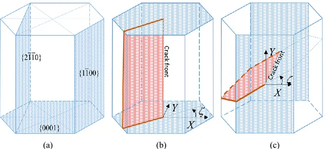
When the crack is inclined with an angle 𝜁 relative to crystallographic planes, as illustrated in Figure 10 for an HCP crystal structure, a change of base for the stress tensor is necessary. Hence, the trigonometric function 𝑓 and the coefficients 𝐴1, 𝐴2 and 𝐴3 are not only

dependent of the second polar coordinate 𝜃 but also of the crack inclination 𝜁 such that 𝐴1(𝜁) = 𝑆11cos2 𝜁 + 𝑆12+ 𝑆22sin2 𝜁 + 1 2(𝑆16+ 𝑆26) sin 2𝜁, (26) 𝐴₂(𝜁) = 𝑆11sin2 𝜁 + 𝑆12+ 𝑆22cos2 𝜁 − 1 2(𝑆16+ 𝑆26) sin 2𝜁, (27) 𝐴₃(𝜁) = (𝑆11− 𝑆22) sin 2𝜁 + (𝑆16+ 𝑆26) cos 2𝜁. (28)

(34)

20

(a) (b) (c)

Figure 10: a) Basal and prismatic planes in an HCP crystal. b) Crack plane (in red) orthogonal to the basal planes (in blue) with an inclination angle 𝜁 relative to {11̅00}

planes c) Crack plane (in red) orthogonal to prismatic planes of the {11̅00} family (in blue).

The TDGL equation, presented in Eq. (15), is chosen to be solved in order to determine the evolution of the structural order parameter and, therefore, predict the possible microstructural changes induced by the presence of a crack in the system. Dimensionless coefficients are introduced as, 𝜂 = √|𝛼0| |𝛽| Φ, 𝑟 = √ 𝑔 |𝛼0|𝜌, 𝑥𝑖 = √ 𝑔 |𝛼0|𝑥̃, 𝑟𝑖 0 = √ 𝑔 |𝛼0|𝜌0, 𝑡 = 1 |𝛼0|𝐿𝜏 in Eq. (21) so that Eq. (15) becomes

𝜕Φ

𝜕𝜏 = ∇̃2Φ − (𝐴 Φ + sgn (𝛽) Φ3+ 𝜅 Φ5), (29)

where 𝐴 = sgn (𝛼0) − √𝜌_𝜌0𝑓(𝜃, 𝜁) and ∇̃ is the dimensionless gradient operator resulting

from non-dimensionalization.

5.2.2 Model 2

The second model is a pilot model for the formation of hydrides in metals, which takes the swelling of the second phase into account. The coordinate system is defined to be Cartesian and plane strain is assumed. A non-conserved phase field variable scalar 𝜑 is selected to describe the evolution of the phases. It is defined so that 𝜑 = −1 characterizes the prevalence of the solid solution, and 𝜑 = 1 corresponds to the hydride dominancy.

Here, the total energy of the system with a volume 𝑉 is the sum of the bulk free energy, which includes a fourth order Landau potential as

ϕ_{𝑏𝑢𝑙𝑘} = 𝑝 (−1 2𝜑2+

1

(35)

21

where 𝑝 is proportional to the height of the double well, the gradient energy F_{𝑔𝑟𝑎𝑑} = ∫𝑔₂(∇𝜑)2_{𝑑𝑉 and the elastic-strain energy}_F

𝑒𝑙 as introduced in section 4.2.1. The

swelling of the hydrides induces a deformation of the material and is taken into account in the total strain 𝜀_𝑖𝑗𝑡𝑜𝑡 as

𝜀_𝑖𝑗𝑡𝑜𝑡 _{= 𝜀}

𝑖𝑗𝑒𝑙+ 𝜀𝑖𝑗𝑠ℎ(𝜑), (31)

where ℎ(𝜑) = 1₄(−𝜑3_{+ 3𝜑 + 2). The presence of solid solution implies ℎ(−1) = 0, and}

that of the hydride induces ℎ(1) = 1, a local maximum of the function. The strain field 𝜀_𝑖𝑗𝑠 designates the strain tensor relative to hydride swelling in the global coordinate system. The energy release in form of material dilatation during phase transformation is embedded in the elastic-strain free energy. The functional derivative of the latter with respect to the phase field variable can, thus, be formulated as,

𝛿F_𝑒𝑙

𝛿𝜑 = ∫ − 3

4𝜎𝑖𝑗 ′ 𝜀𝑖𝑗𝑠 ′(1 − 𝜑2) 𝑑𝑉 (32) The expansion is anisotropic and the directions of the eigenstrains, 𝜀₁₁𝑠 ′_{𝑎𝑛𝑑 𝜀}

22𝑠 ′, relative to the

swelling are assumed to be the directions of the principal stress 𝜎₁₁ ′ _{and 𝜎}

22 ′ . The tensors 𝜀𝑖𝑗𝑠 ′

and 𝜎_𝑖𝑗 ′_{are related to}_𝜀

𝑖𝑗𝑠 and 𝜎𝑖𝑗 respectively through 𝜀𝑝𝑞𝑠 ′ = 𝑄𝑖𝑝𝑠 𝑄𝑗𝑞𝑠 𝜀𝑖𝑗𝑠 and 𝜎𝑖𝑗 ′ = 𝑄𝑖𝑝𝑠 𝑄𝑗𝑞𝑠 𝜎𝑖𝑗.

where 𝑄_𝑖𝑝𝑠 _{and 𝑄}

𝑖𝑝𝑠 are basis transition matrices. The components of 𝜀𝑖𝑗𝑠 ′ are directly provided

from the literature and, 𝜎₁₁ ′ _{and 𝜎}

22 ′ are the eigenvalues of 𝜎𝑖𝑗.

The problem is driven by the minimization of the energy as the mechanical equilibrium is satisfied at all times. The governing equations are, therefore, the second law of Newton for static conditions and the TDGL equation, Eq. (15). By using the derivative of the different energy contributions with respect to 𝜑, the TDGL equation can be written as,

1 𝐿 𝜕φ 𝜕𝑡 = − [(− 3 4𝜎𝑖𝑗 ′𝜀𝑖𝑗𝑠 ′− 𝑝𝜑) (1 − 𝜑2) − 𝑔∇2𝜑] . (33)

5.3 Numerical methods

5.3.1 Model 1

The simulations of the microstructural evolution of isotropic and HCP materials, which are described with the first presented methodology, are performed through the use of the software FiPy (Guyer, et al., 2009). With this Python-language-based module, the TDGL is solved based on a standard finite volume approach over a grid composed of equally-sized square elements. The solver employs a LU-factorization solving algorithm, which allows the results to converge rapidly. The domain is considered large enough so that it prevents edge-effects on the results.

(36)

22

The numerical set-up utilizes a 1000 × 1000-element grid with an element dimensionless side length of ∆𝑙̃ = 0.2 for the isotropic body and a 200 × 200-element grid with a ∆𝑙̃ = 0.5 in the case of a HCP material. The time stepping is respectively taken as ∆𝜏 = 0.1 and ∆𝜏 = 0.05.

A zero gradient of the order parameter is applied perpendicular to the boundary implying a non-variation condition of the phase field variable at the domain limits. The phase dynamics is triggered by an initial random distribution of the order parameter value over the grid in the range [0.5, 1] ∙ 10−4_.

5.3.2 Model 2

The second model presented in section 5.2.2 employs the finite element method to solve the fully coupled mechanical and the phase transformation problem. The software Abaqus (Dassault System, 2009) is selected because it allows using user subroutines to alter the code. Thus, the fully coupled thermo-mechanical problem is modified and adapted for phase field modeling.

Equation (33) undergoes a backward-difference scheme and the solution of the non-linear system is obtained through the use of Newton-Raphson’s method, which includes a non-symmetric Jacobian matrix, as

[𝐾_𝐾𝑢𝑢 𝐾𝑢𝜑 𝜑𝑢 𝐾𝜑𝜑] [ ∇𝑢 ∇𝜑] = [ 𝑅_𝑢 𝑅_𝜑] , (34)

where ∇𝑢 and ∇𝜑 are the correction for incremental displacement and order parameter, 𝐾_𝑖𝑗 are the “stiffness” sub-matrices of the Jacobian matrix and 𝑅𝑖 are the residual vectors for the

mechanical and the phase evolution parts of the system.

The equations are first solved simultaneously over a 300 × 300 grid of equally-sized and quadratic elements with an element side length ∆𝑙 = 1μm for a defect-free hydrogenated plate. Regarding the boundary conditions, a zero displacement condition along 𝑥⃗⃗⃗⃗ is applied ₂ to the lower edge and the first element of the same edge is also blocked in displacement along the 𝑥⃗⃗⃗ . The load is induced by a displacement imposed on the upper edge of the domain with ₁ a determined rate. An additional zero phase-field gradient is applied on the whole boundary. For all simulations performed on the plate the same initial condition is applied to the computing domain as a Gaussian distribution of the order parameter within the range [−0.04,0.01]. Finally, an adaptive time increment is employed and is initially equal to 10−7_s.

Later, Eq. (33) is solved over a meshed domain accounting for a notched plate. The same side length is used for the elements of the notched plate as the one used with the plate mesh. The notch, which has a root radius of 0.3 mm as in (Ma, et al., 2006) penetrates the plate in the direction 𝑥⃗⃗⃗⃗ from the upper edge. The left edge is fixed while a displacement in the direction ₂ 𝑥₁

⃗⃗⃗ is applied on the right edge. The other edges are free from mechanical boundary conditions. A zero-gradient of the order parameter is also applied on the boundary of this

(37)

Results and summary of appended papers

23

geometry. For this simulation, as for the plate, the order parameter is initially distributed within the range [−0.04,0.01] over the domain and the adaptive time stepping, whose initial value is 10−7_{s, is used.}

6 Results and summary of appended papers

The attached papers describe either Model 1 or Model 2 as well as the respective numerical procedures. Simulations were performed for specific situations with both models and the results are presented in this section.

6.1 Paper A

In the first paper, Model 1 is applied to isotropic bodies at a temperature T. A parametric study is achieved and presented showing different situations which can be modeled with this formulation. The influence of the system total free energy coefficients, presented in Eq. (21), on the solution of Eq. (29), and the modification, or shift, of the phase transition temperature by the crack-induced stress gradient are thoroughly discussed.

6.1.1 The analytical steady-state solution

First, Eq. (29) is analytically examined for a steady state and for a condition implying that the variation of the order parameter in one point does not affect its neighbors, i.e. 𝜕Φ 𝜕𝜏⁄ = 0 and ∇̃2_{Φ = 0. One result of this investigation is the phase diagram, illustrated in Figure 11, which}

exhibits the dimensionless distance from the crack tip versus 𝜅 sgn (𝛽) for 𝛼₀ > 0 or 𝑇 > 𝑇_𝑐₀, i.e. in the cases where no phase transformation is expected to occur under defect-free conditions.

Figure 11: Phase diagram for steady-state and no order parameter gradient conditions for

𝛼0 > 0. The notations I and II denote respectively the solid solution and the second phase. The superscript (*) indicates a metastable state of the considered phase.