An approach to evaluate machine learning algorithms for appliance classification

(1)

An approach to evaluate machine

learning algorithms for appliance

classification

A low-cost hardware solution to evaluate machine

learning algorithms for home appliance classification in

real time

David Hurtig

Charlie Olsson

Computer and Information Science Bachelor

15 credits Spring 2019

Date for final seminar: 2019-05-31 Supervisor: Radu-Casian Mihailescu Examiner: Reza Malekian

(2)

(3)

Abstract

A cheap and powerful solution to lower the electricity usage and making the residents more energy aware in a home is to simply make the residents aware of what appliances that are consuming electricity. Meaning the residents can then take decisions to turn them off in order to save energy. Non-intrusive load monitoring (NILM) is a cost-effective solution to identify different appliances based on their unique load signatures by only measuring the energy consumption at a single sensing point. In this thesis, a low-cost hardware platform is developed with the help of an Arduino to collect consumption signatures in real time, with the help of a single CT-sensor. Three different algorithms and one recurrent neural network are implemented with Python to find out which of them is the most suited for this kind of work. The tested algorithms are k-Nearest Neighbors, Random Forest, and Decision Tree Classifier and the recurrent neural network is Long short-term memory.

(4)

(5)

1 Introduction

In this section, we will first give a brief explanation of some necessary terms for

understanding this thesis. We will then look at the background that has been conducted in the same field as this research.

In this thesis, we have chosen to group k-Nearest Neighbor, Random Forest, and Decision Tree Classifier as “Group-A” and Long short-term memory will be grouped as “Group-B”. Although LSTM could be seen as a sort of machine learning algorithm, we have chosen to separate it from the other algorithms depending on the different ways to implement it and for readability purposes. The collective word for Group-A and Group-B will be “machine learning algorithms”.

1.1 Different types of machine learning

Andriy summarized machine learning with one sentence in his book “The Hundred-Page Machine Learning Book” by saying: “Machine learning is a subfield of computer science that is concerned with building algorithms which, to be useful, rely on a collection of examples of some phenomenon. These examples can come from nature, be handcrafted by humans or generated by another algorithm” [1]. He then continues with: “Machine learning can also be defined as the process of solving a practical problem by 1) gathering a data set, and 2) algorithmically building a statistical model based on that data set. That statistical model is assumed to be used somehow to solve the practical problem”. The term “machine learning” is quite broad and there are many subsets of it. Therefore, this thesis does not focus on explaining machine learning so we will just give a brief

explanation of some of the parts that are necessary to get a basic understanding of machine learning.

1.1.1 Supervised learning

In supervised learning, the labels are known in the so-called training data set. Since the labels are known, the goal of this kind of machine learning is to produce a model that takes an unknown input where the label is not known and then output the appropriate label which the model think this new unseen data is. Supervised learning can be further divided into two parts:

• Classification, which is the organization of labeled data.

• Regression, which is the prediction of trends in labeled data to determine future outcomes.

1.1.2 Unsupervised learning

Unsupervised learning is the opposite of supervised learning in the way that the labels are not present in the training data set. The goal here is to model the underlying structure in the data in order to learn more about the data and then draw conclusions from the data. In unsupervised learning there are 4 different kinds:

(9)

2

• Association, to discover rules that describe large portions of the data. • Anomaly detection automatically finds unusual data points of the data. • Autoencoders, takes input data and compress this into code and then tries to

recreate this input data from the code.

1.2 Nonintrusive vs intrusive load monitoring

In this section, we will describe the two different kinds of load monitoring methods, nonintrusive load monitoring, and intrusive load monitoring.

1.2.1 Nonintrusive load monitoring

Nonintrusive load monitoring (NILM) (sometimes called nonintrusive appliance load monitoring) was first proposed by George W. Hart [2]. NILM is the process of identifying individual appliances that switch on and off independently running inside a house and monitor their energy usage from a single sensing point. Georges basic idea was to place one sensor between the electricity meter and its socket in order to see and capture changes in the voltage and current that a house consumes in high detail. This collected aggregated load data can then be analyzed and matched against previously collected load signatures on appliances. Since this method doesn’t require individual access to all the individual appliances to install separate sensors, it can be both a convenient and a very cost-effective way to collect and analyze load data. All of this usually means that NILM has simple data-gathering hardware but often a complex software for signal processing and analysis. This is because mathematical algorithms must separate the measured load into separate components. The NILM approach also allows simple installation,

maintenance, and removal of the hardware.

1.2.2 Intrusive load monitoring

Intrusive load monitoring (ILM) in contrast to Nonintrusive load monitoring, is a

distributed sensing system meaning it requires individual sensors for each and every device in the house that should be monitored and detected [3]. This can, for example, be

achieved with the help of wireless smart plugs that sends the monitored data to some kind of central hub. It means that ILM often consist of more complex data-gathering hardware where it’s necessary to use multiple data-gathering hardware for every single appliance, but very simple software.

1.3 Background

Many different approaches have been tested and documented using NILM to classify unknown appliances and the success rate seem to vary quite a lot. In this section, we highlight some of the recent work in this field and we only focus on the previous research that has been done with the help of machine learning to classify appliances.

(10)

3

In “Electric appliance classification based on distributed high-resolution current sensing“ [4] the writers achieved great results with their system in terms of accuracy of how well they managed to identify appliances. They used a low-cost distributed system that they had developed earlier called SmartMeter.KOM [5]. They used it to gather power consumption from individual appliances at a sampling rate of 1.6kHz, extracted features from the data collected, and then wirelessly transmitted the features to a local classification server. They analyzed both the initial state current when an appliance turns on as well as the steady-state currents to help in the classification. They used a supervised machine learning approach with over 3400 load signatures of 16 different types of appliances and one model of each appliance type which achieved a result with an accuracy of 100% using the initial current and steady state combined with Bayesian Network Classifier. However, they did not take into account that the same type of appliance may have slightly different power consumption depending on what brand or model it is. This is something that may greatly reduce the accuracy of their model since only using one model per appliance to train their machine learning algorithm will not be representable of the real world.

“Machine learning approaches for electric appliance classification” [6] are focusing on acquiring the data from the appliances at a low frequency at the rate of 0.1Hz and with the help of smart outlets called PLOGGs. They then with the help of a computer store this acquired data in a database. They used a supervised machine learning approach and tested two different algorithms: K-Nearest Neighbor got an accuracy of 85% and Gaussian Mixture Model also got an accuracy of 85%. This research used five different kinds of appliances and six different models and brands of each appliance. The researchers stated that real time identification is not their priority since the smart outlets are

collecting samples at such low frequency. By using PLOGGs it seems to be a combination between ILM and NILM since it doesn’t have the single sensor point.

In “Low-cost real-time non-intrusive appliance identification and controlling through machine learning algorithm” [7] they focus on identifying the appliances fast after it has been turned on. This means that they are measuring energy consumption at a fast rate, although they don’t mention how fast. They identify the appliance in real time by only looking at the initial current consumption when an appliance is turned on and not its steady state. This also means that they can successfully identify multiple appliances running at the same time as they are turned on, but not if they start the sensor during when the device is already turned on. Four different kinds of appliances were used but they did not mention how many load signatures from these appliances that were used for training the machine learning algorithms nor did they mention if they used exactly the same appliances for testing and training. Their results show that k-Nearest Neighbor achieved 85 % accuracy and Random Forest 89 % respectively.

“Real-Time Recognition and Profiling of Appliances through a Single Electricity Sensor” [8] proposed a system called RECAP (Recognition of electrical appliances and profiling in real time) that is using a single wireless current sensor to measure the electric load at a sampling rate of one value per minute. This means they can’t give fast real time feedback to the user of what appliances it is that is running. They have a big focus on developing

(11)

4

something that could be deployed outside of a testing environment and therefore they also built a GUI for users to record data from their own appliances one by one. This collected data can then be used for training a machine learning algorithm which can then classify the same recorded appliances in the future. They tested their system in a testing environment in the form of a kitchen and it was tested on four different kinds of

appliances where they achieved an accuracy of 84% with an Artificial Neural Network.

The writers in “Automatic recognition of electric loads analyzing the characteristic parameters of the consumed electric power through a Non-Intrusive Monitoring methodology” [9] went a slightly different route compared to other papers and did not collect any data with sensors. Instead, they used an existing database called ACS-F2 [10] for training and testing of their machine learning algorithms. They divided their testing into two different parts. In the first part, they tried to identify one appliance at a time, given eight appliances. The algorithms Decision Tree Classifier, k-Nearest Neighbor, Discriminant Analysis and a Feed-forward Neural Network was chosen for this and the results showed that Decision Tree Classifier was the most accurate and gave an accuracy of 99%. In the second part, they tried to identify what appliances were running when three different appliances were running simultaneously. For this, they used a Feed-forward Neural Network and overall achieved a result of 98% accuracy. They did not do any physical testing of their algorithms.

“Classification of ON-OFF states of appliance consumption signatures” [11] also tested their classification on the ACS-F2 database. They divided the database into different parts to test different things. For example, they tested if it's always better with more features, meaning more potential information about the load signature. They tested both with 8 and 30 features and the results showed that 8 was actually better in this particular case. They did not reflect over why this was results. Random Forest was the best

algorithm and achieved 93.78% accuracy, Bayes Net was in the middle with 88.96% accuracy and the worst performer was Hoeffding Tree which gave an accuracy of 83.94%. This research didn’t do any physical testing at all.

In “Identifying Outlets at Which Electrical Appliances Are Used by Electrical Wire Sensing to Gain Positional Information About Appliance Use” [12] the focus is on identifying where in the home one type of appliance is being used. In this paper, they identify what kind of appliance that is running with the help of one current sensor collecting data at a rate of 2kHz and use a Decision Tree Classifier to identify the appliance. They tested on 16 appliances and achieved an average F1-score of 92 %.

“An Approach of Household Power Appliance Monitoring Based on Machine Learning” [13] evaluated a multi-class Support Vector Machine on 11 different appliances in one home. It gave a result of 90 % accuracy though it should be noted that they seem to have trained and tested their algorithm on the same appliances which might not be representative of a real world scenario.

(12)

5

1.4 Problem

There are multiple studies done in the same research field as mentioned in section 1.3 Background. They all differ in some ways, but there has not been any research that has focused on testing multiple different machine learning algorithms to determine the best in terms of accuracy, while also applying it in a real world scenario to quickly classify

physical appliances at any time during its load signature.

As mentioned earlier most of these studies have been inconclusive or have focused on different ways to measure and how to measure the electrical load signature. What we are trying to do in this thesis is to examine different machine learning algorithms to decide which one will return the highest accuracy in a theoretical environment and then implement it with our prototype system. As also mentioned above in section “1.3

Background” previous work has not tested their system physically but only theoretically in software with data sets.

1.5 Purpose

The purpose of this thesis is to examine the possibility to correctly detect and classify six different home appliances based on their electrical load signatures with the help of

machine learning algorithms. We wanted something that is low-cost, easy to purchase and set up, and could also be expanded for more devices in the future. The system should also work on physical devices in real time. More importantly, it should be possible to identify the appliance anytime when it is on, meaning that the system should not need to have been collecting data since the start of the appliance or collect all the data until the appliance turns off.

1.6 Research question

The research question derived from this mentioned problem and purpose, therefore, is: What is the best performing machine learning algorithm for appliance classification? And to answer this question we also propose: A low-cost hardware solution to evaluate machine learning algorithms for home appliance classification in real time.

(13)

6

2 Method

The method that we used in this thesis is based on NILM that was explained in section 1.2.1 Non-intrusive load monitoring. NILM is about identifying multiple individual

appliances with one sensor by looking at the current and voltage [2]. The method used in this thesis is not a direct copy of NILM since this system cannot differentiate between multiple appliances running at the same time. This is a fundamental thing with NILM. However, we still considered the method as NILM because most of the other steps that we are doing are the same as used in NILM.

In this section, we give detailed information about the different selected appliances for this thesis and then explain how we have chosen to implement the different steps in NILM. These steps are to collect load signatures, analyze these load signatures and then to classify the appliances using supervised machine learning. We also describe the different ways we have measured accuracy for the different machine learning algorithms.

2.1 Different types of appliances

Different kinds of consumer appliances can generally be divided into three different categories that were proposed by [2]. However, these three categories were later on revisited and updated to add one more type of category by [14], bringing it up to four different categories of appliances. Below is a short description of the different kind of appliances and how they differentiate from each other.

2.1.1 Type-I

ON-OFF appliances are appliances that only have two states, either ON or OFF. The time that these types of appliances are being run does not matter since its load signature will always look the same. Examples of some of these are toasters or non-dimmable lights.

2.1.2 Type-II

Finite state machines (FSM) are multi-state appliances that have a finite number of operation state. This means that the appliance can have multiple states and therefore it consumes different amounts of energy during its entire cycle. The patterns of these appliances are repeatable. To collect an entire load signature from these appliances they need to be run their entire cycle. Some examples of devices are microwaves, dishwashers or washing machines.

2.1.3 Type-III

Continuously variable appliances are appliances that have constantly varying power consumption in their ON-state. These appliances do not have a number of fixed states and therefore they don’t show any periodic patterns which mean that they are very hard to identify correctly [14], [15]. Examples of these type of appliances could be dimmer lights or power drills.

(14)

7

2.1.4 Type-IV

Permanently on appliances are appliances that are constantly on throughout long periods of time and constantly consuming energy. Examples of this kind of appliances could be landline phones or alarms.

2.2 Electric Load

There are three kinds of circuits in electrical devices, resistive, inductive and capacitive. These different circuits differ in the way that they consume AC power and what the energy is transformed to [16].

2.2.1 Resistive load

Resistive loads are usually used for heating, e.g. toasters. Resistive load works by obstructs the flow of the electrical energy and therefore the current in the circuit is converted into thermal and light energy. The voltage and current waves are “in phase” relative to each other.

2.2.2 Inductive load

Inductive Loads are usually used for devices that have moving parts e.g. vacuum cleaners. These loads use a magnetic field to do the work. This type has a coil that stores

magnetic energy when current is passing through it. The voltage and current wave are “out of phase” causing the current wave to “lag” behind the voltage wave.

2.2.3 Capacitive load

Capacitive loads do not exist in a stand-alone format, therefore, it is not used as a classification. The capacitive load is almost the opposite of the inductive load. A

capacitive load stores electrical energy but this time the current and voltage wave is also “out of phase” but the current wave is “leading” the voltage wave.

2.3 Selected appliances

The different appliances and some additional information that was chosen for this thesis are described below in table 1. Below the table, there is an overview of each appliance used in this thesis. In graphs 1-6 below, there is a visualization for one device per appliance entire load signature.

(15)

8

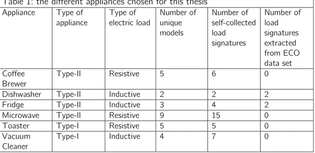
Table 1: the different appliances chosen for this thesis

Appliance Type of appliance Type of electric load Number of unique models Number of self-collected load signatures Number of load signatures extracted from ECO data set Coffee Brewer Type-II Resistive 5 6 0

Dishwasher Type-II Inductive 2 2 2

Fridge Type-II Inductive 3 4 2

Microwave Type-II Resistive 9 15 0

Toaster Type-I Resistive 5 5 0

Vacuum Cleaner

Type-I Inductive 4 7 0

Here is an explanation of why these particular appliances were chosen for this thesis and also the settings that were used for that particular appliance if it had multiple settings.

• Coffee brewers can vary quite a bit in their energy consumption depending on brand and model, therefore coffee brewers were chosen. The coffee brewers in our data set have ON, OFF and “keep warm”-state which seems to be the most common way a coffee brewer works. The load signature seemed to change somewhat depending on how much coffee we brewed, therefore we brewed anything between two and six cups during data collection.

• Dishwashers were chosen because it has a very long cycle of approximately 3 hours, and since it’s a Type-II appliance, it is not consuming constant power during this time. This was the appliance that was the most difficult to get data from since we didn’t have access to many dishwashers. Most of the modern dishwashers have different washing modes to choose from. This setting was put on ECO since it was the default mode that the owners always used.

• Fridges were chosen because of its very long load signatures. Unfortunately, it was very hard to get access to different fridges of different brands and therefore our own collected data is a bit limited in size.

• Microwaves were chosen because we had easy access to multiple different models and therefore, we wanted to evaluate if this would increase its accuracy in the classification. Most microwaves have multiple settings for a different kind of usage and for this thesis we only recorded data when the setting was on 700 watts. The time of which it was running was between 20 seconds to 5 minutes. During our data collection, we concluded that no new consumption patterns would emerge the longer it was running, therefore it was not necessary for us to collect data for a longer period of time. It should also be noted that some microwaves had lamps that turned on when the door was opened and in this thesis, the microwaves lamp usage is not classified as the appliance is turned on.

(16)

9

• Toasters were chosen because it is very repeatable in its consumption pattern between different brands and models and we wanted to see if this would increase its accuracy in the classification. Many toasters have some kind of settings that allows the user to set how long the bread should be toasted, this setting doesn’t influence energy consumption for the toasters tested for this thesis. The setting was set to the middle value of every toaster.

• Vacuum cleaners were chosen since we wanted to have two kinds of Type-I appliances and it’s a common household appliance. It has a steady state in its consumption but the difference between different models can vary greatly and therefore we saw this as a great opportunity to test the accuracy of the

classification. Many vacuum cleaners have different settings depending on what surface is going to be cleaned. During our data collection, we always put the setting to hardwood floors.

(17)

10 Graph 1: Shows the entire load signature of a

coffee brewer.

Graph 2: Shows the entire load signature of a dishwasher.

Graph 3: Shows the entire load signature of a fridge.

Graph 4: Shows the entire load signature of a microwave.

Graph 5: Shows the entire load signature of a toaster.

Graph 6: Shows the entire load signature of a vacuum cleaner.

2.4 Data Acquisition

In this section, we will describe how we collected data, how our low-cost hardware platform was built, what it consisted of and the cost for each of its parts. We will also discuss a data set used to fill out some missing data.

(18)

11

2.4.1 Data acquisition from physical appliances

To be able to collect and record the load signatures from the different appliances, a prototype hardware platform was developed and associated software for it was written. There are multiple different ways to obtain this data. Both [6] and [4] used smart outlets on individual appliances for this task. The choice fell on to develop an Arduino based platform very similar to the one used in [7]. We chose a Current transformer (mentioned as CT-sensor in this thesis) with a precision of 98% [17] to measure the alternating current in our prototype. This sensor could easily be used if this work was further evolved from prototyping in a lab environment to actually be deployed in a real world

environment.

The CT-sensor can measure the current that an appliance is consuming because a wire that is carrying an electric current creates a magnetic field around it. In short, this means that the CT-sensor together with a burden resistor generates a low-voltage that the Arduino analog input can receive and then the code that is running on the Arduino can translate this voltage into amperes. The CT-sensor needs to be clamped around a single current-carrying wire which is why we needed to split our extension cord as can be seen in figure 1. If the CT-sensor would be clamped around multi-core cables it would not work properly since it would measure the sum of the current flowing in opposite directions, as it does with AC electricity, which would always result in zero.

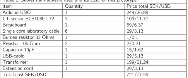
Table 2: Shows the hardware used and its cost for this prototype

Item Quantity Price total SEK/USD

Arduino UNO 1 249/26.89

CT-sensor ECS1030-L72 1 109/11.77

Breadboard 1 59/6.37

Single core laboratory cable 6 29/3.13

Burden resistor 33 Ohms 1 1/0.1

Resistor 10k Ohm 2 2/0.21

Capacitor 10µF 1 15/1.62

USB-cable 1 29/3.13

Transformer 1 199/21.24

Extension cord 1 29/3.13

Total cost SEK/USD - 721/77.59

This total cost, as can be seen in Table 2, does not include the PC where the data values are processed and then classified as the predicted appliance. Figure 1 below is an image of the setup described in Table 2.

(19)

12

Figure 1: 1) CT-sensor connected to an extension cord which has been cut open to reach the necessary cable. 2) USB cable connected to the PC. 3) Arduino running EmonLib, reading the CT-sensor and sending it to the PC. 4) Extension cord where we connect the appliances.

As mentioned earlier the Arduino needs to be running some code that can translate the low-voltage from the CT-sensor into amperes. To do this we used an open source library that is supplied by OpenEnergyMonitor [18] called EmonLib [19]. EmonLib is a library that can be used for energy monitoring and we used it for converting the low-voltage value from the CT-sensor that is connected to the Arduino into amperes. To calculate apparent power, it’s also necessary to have the voltage and to solve this we hardcoded the voltage to 230 volts. The volt may vary depending on what the specific country has as standard but since this thesis is conducted in Sweden, we used 230 volts. Hardcoding the voltage will not give 100% true accuracy on apparent power since voltage, in reality, may fluctuate [20].

The EmonLib running on the Arduino works by calculating the average of 300 values coming from the CT-sensor and then returns this average as the apparent power. For this thesis, we have focused on a relatively high sampling rate at 50 Hz to gain more

information about the appliances, which is 50 data points per second. This high sampling rate gave us access to a large number of data points in a small timeframe and increased the chances of seeing detailed patterns we would otherwise miss which in turn might help in the classification of the appliance. The data points constantly get sent from the Arduino to a PC through a USB-cable. The different appliances were run one by one and a Python script was then collecting the data and saving it in a .CSV file. A low threshold

(20)

13

was set in the Python script so the saving of data would only start when the value of the apparent power was above this threshold. This was done to avoid small unwanted

disturbance in the electrical signals coming from the prototype platform. In the graphs above (graph 1-6) there are examples of the raw data acquired from every type of appliance. Please note that the X-axis is very different in size since some appliances have extremely short load signatures to others.

2.4.2 Electricity Consumption & Occupancy data set

As we can see in table 1 there were very few devices and therefore unique load signatures collected from fridges and dishwashers. Only 2 from fridges and 4 from dishwashers. This is because these two appliances were the most difficult to get a hold of. They also have very long cycles which made it very time consuming to collect data. Because of this, it was decided that we would also take help from an accessible online data set called Electricity Consumption & Occupancy (will be referred to as ECO data set in this

thesis)[21], [22] to extract more data for fridges and dishwashers. ECO data set contains measures of apparent power from different appliances at the sampling rate of 1 Hz. This was not even close to our own sampling rate, which was 50 Hz, meaning that some detailed data was missed. Considering the load signatures of dishwashers and fridges, in graph 2 and 3, they have very long load signatures that hardly changed so we decided that ECO data set would help since our high sampling rate gave the same mean as ECOs slower sampling rate. The only negative thing was that we would miss possible initial current spikes, but it was better to get more fridges and dishwashers to avoid underfitting the algorithms in Group-A.

2.5 Feature extraction

In this section, we will discuss how we processed our data and how we did to extract features for Group-A and Group-B.

2.5.1 Sliding window

We used a sliding window approach first to divide an entire appliance load signature into smaller subsets of data points. This technique has also been used in [12]. We were dealing with time series data that generated a different amount of data depending on which device that was being measured. For example, a coffee brewer probably won’t brew coffee for three hours straight, but the dishwashers that were used for collecting data was on for three hours. Because of this, the technique to divide the raw data into smaller subsets with the sliding window worked very well. Multiple different sliding window sizes were tested for both Group-A and Group-B to find the most optimal size for each set. A larger sliding window size was used fridges and dishwashers because both fridges and dishwashers had very long load signatures and we noticed that a small window for these devices only leads to more data that looked the same. The sliding window size is a fine balance since we wanted it to be as small as possible so that the system wouldn’t have to collect data for too long when classifying appliances in real time but not too small so that the data represented to few data points and made it harder to classify.

(21)

14

The sliding window worked in the way that it “slides” over the raw data acquired from the sensor and then extracts/calculates our selected features from this data and then keeps on “sliding” forward in the data point sequence. Using an approach like this sliding window technique gave us detailed information about the way that an appliance is consuming energy.

2.5.1.1 Group-A

The sliding window size used in Group-A was 1000 data points which are equal to about 20 seconds of data collection. This means that an appliance needed to run for at least 20 seconds before the system has collected enough data to classify the device. For fridges and dishwashers, we used a sliding window size 6 times larger, i.e. 6000 data points. From the ECO data set, we used a 120-second window since that equals to 6000 of our own data points. The size of the sliding window was determined from an experimental study which is described in section 4.1.1 Size of the sliding window and preventing overfitting. In graphs 7-12 below there are examples of the first sliding window for each appliance during their startup in Group-A.

(22)

15 Graph 7: Shows the first 1000 data points of a

coffee brewer

Graph 8: Shows the first 6000 data points of a dishwasher

Graph 9: Shows the first 6000 data points of a fridge

Graph 10: Shows the first 1000 data points of a microwave

Graph 11: Shows the first 1000 data points of a toaster

Graph 12: Shows the first 1000 data points of a vacuum cleaner

2.5.1.2 Group-B

The sliding window size for Group-B was set to 100 data points which equal to about 2 seconds of data. To keep the consistency with Group-A we chose to have the fridge and dishwashers 6 times as large, i.e. 600 data points which equals to 12 seconds. From the ECO data set, we used the same time-span i.e 12 seconds of data. The size of this sliding window was also determined from an experimental study which is described in section 4.2.1.1 Hyperparameters graphs.

(23)

16

2.5.2 Feature selection

A feature is an attribute that is extracted from each of the sliding windows. This attribute is either a unique number, such as the highest value or a result of a mathematical

calculation, e.g. mean value, for each sliding window. These attributes were used in each sliding window to remove the time aspect that would otherwise exist and allow for a more flexible data set. This means that the CT-sensor technically can be hooked up at any time when an appliance is turned on and it does not necessarily need to be collecting data at the start of the appliances cycle since in the training data we have divided the load signatures into smaller parts with the help of sliding windows.

The features chosen to extract from each sliding window was the following: • Highest value.

This feature was particularly useful when different appliances “spikes” during their startup state. A few of the appliances did this which can be seen in the graphs 7-12 above.

• Lowest value.

If an appliance shows repeatedly lows and highs in its load signature this feature helped this particular appliance stand out from the rest which greatly enhances the classification accuracy.

• Mean value.

This feature was a good way to know how much energy the appliance is consuming on average and therefore help it to stand out from the rest. • Standard deviation.

This feature was helpful to know if the measured appliance is in its steady state. The standard deviation shows the dispersion of the numbers. If the standard deviation value is low, it means that most of the values in the sliding window is close to the mean value and the appliance is probably in its steady state. This was helpful since it will give a similar number each time the sliding window is in steady state.

2.6 Theoretical appliance classification

When we had collected all possible raw data from available appliances and features had been extracted from this data it could finally be used for classifying an appliance. Since we used a supervised learning approach the machine learning algorithms know what kind of appliance it is in the training data. An example of how the data looks for the machine learning algorithms in a .CSV file after the features had been extracted from the sliding windows can be seen below.

class,maximum,minimum,mean,standard_deviation coffee,1050.9,869.89,976.98,52.96 dishwasher,439.02,63.68,117.65,18.38 fridge,166.17,132.75,150.28,8.59 micro,1446.45,1130.17,1336.16,97.89 toaster,757.83,644.53,703.08,38.38 vacuum,2096.56,1645.45,1915.4,149.31

(24)

17

There was more than one instance for each appliance in the .CSV file, but this shows a good overview of the data that the machine learning algorithms were trained on and how they are different for the different appliances when the features were extracted. In the testing data, the class was unknown during the classification and then after the algorithm has classified to what it thinks it is, the correct class was revealed.

2.6.1 Group-A

We used a popular open-source machine learning Python library called scikit-learn [23] for implementing Group-A. When Group-A was evaluated with F1-score the splitting of the total amount of data was 90 percent for the training set and the rest 10 percent for testing data. The size of this split was relatively low for the test size, but this was necessary since we had a low amount of collected data to work with. For the cross-validation accuracy, the number of folds was set to 5. To read more about F1-score see section 2.9.6 F1-score and to read more about cross-validation see section 2.9.3 Cross-validation.

2.6.2 Group-B

For implementing long short-term memory we used an open source machine learning library called Tensorflow [24] together with Keras API [25]. For evaluating LSTM, we didn’t use F1-score but instead only used cross-validation with the number of folds set to 5.

2.7 Real time appliance classification

We tested our real time prototype on the algorithms from Group-A. Considering the sliding window size used we could, for example, run a physical microwave that was not in the training data set for 20 seconds and then it would have had received enough data to predict the class with Group-A algorithms. When the algorithms had finished the result containing the predicted class as well as the confidence score for each algorithm was printed.

When the system was running in real time it first needed to collect the necessary amount of data points (1000). Then this raw data was sent to a feature extraction method, while the system continued to collect more data in the background. The features were the same as mentioned in section 2.5.2 Feature extraction, but we didn’t use the real time

classification for evaluating the machine learning algorithms since this was done in the theoretical classification part of this thesis. We did look at the confidence score for Group-A to see how confident it was on each classification and to determine whether a certain classification was good enough to be seen as true.

2.8 Machine learning algorithms

There are plenty of algorithms out there that would have been suitable for this kind of research question that we are investigating. Since we had labels on the training data, we used supervised machine learning algorithms. In section 1.3 Background we mentioned

(25)

18

different papers that used different algorithms and from those paper, we have selected what algorithms would be best suited for our kind of data, the features we have used and the way we have structured the data with sliding windows. As previously mentioned in section 1 Introduction, we have separated the algorithms into two different sets. Group-A which includes three different classification algorithms, those are Random Forest, Decision Tree Classifier and k-Nearest Neighbor. Group-B includes one recurrent neural network called LSTM.

2.8.1 Group-A

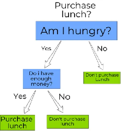
Random Forest and Decision Tree Classifier are based on something called a decision tree. To understand these two algorithms, it is necessary to understand what a decision tree is and how it works. A decision tree is basically a flowchart of questions where the answer to these questions lead to more questions which eventually reaches a decision. For human readability, these questions and answers could be visualized as if-then-this rules from which the flowchart is constructed from [26].

The decision tree begins with the main question, a question which needs a decision. In figure 2 we have for demonstration purposes chosen “should I purchase lunch”. From this, a question, which has a certain amount of possible answers, are asked. In our example, that question is “Am I hungry?”. These answers then lead to more questions until it reaches the end of the decision tree and a decision can be made. In our example the blue squares represent questions, the arrows represent answers to these questions and the green squares represent decisions to the major question on top.

Figure 2: Decision tree visualization. Blue squares represent questions asked, the arrows represent answers to these questions and the green squares represent decisions at the end of the tree.

2.8.1.1 Random Forest

Random Forest (RF) is one of the decision tree based algorithms we chose. RF is based around the idea that multiple, smaller, decision trees are better than one large. Each decision “tree” in the “forest” represents a random number of rows and features and only has access to a random set of the training data points. This gives the algorithm a higher variety of decision trees with different outcomes which gives a more robust overall

(26)

19

prediction. RF takes all the results from each of the trees and looks at which class has the majority and assumes that this is the correct classification [27].

2.8.1.2 Decision Tree Classifier

Decision Tree classifier (DTC) is the second decision tree algorithm that was chosen for this thesis. Compared to Random Forest it only exploits one large decision tree. There are different kinds of Decision Trees but for this thesis, we have chosen Iterative

Dichotomiser 3 (ID3), which is one of the earliest DTC and works by constructing the Decision Tree top-down [26] and then looks at each feature that gives us the highest amount of information to continue the classification. This goes on until the algorithm reaches the end of the tree.

2.8.1.3 k-Nearest Neighbors

k-Nearest Neighbors (k-NN) is an instance based supervised machine learning algorithm [26]. k-NN classifies a new object by looking at its k-number of nearest neighbors from the training data. The algorithm then utilizes a majority vote to look at which class is the majority of the k nearest neighbors and from there assumes that the majority class is the correct classification [28].

There are multiple different ways to measure the distance with k-NN, some more complicated and some are more basic, those include Euclidean, Standardized Euclidean, Mahalanobis, City block, Minkowski, Chebychev, Cosine, Correlation, Hamming, Jaccard, and Spearman [28]. Euclidean is the most straight forward one that simply measures the distance between two points and as proven in [28] there are no major differences in accuracy depending on the distance algorithms.

Figure 3: k-NN visualization. Green square represents a new, unknown object. Red stars and blue triangles represent different classes known. When K=3 the majority class is a star, therefore the new object would be classified as a star. When K=5 the majority objects are triangles, therefore, the new object would be classified as a triangle.

(27)

20

2.8.2 Group-B

Group-B consists of one recurrent neural network called Long short-term memory (LSTM). A recurrent neural network is a kind of neural network. A neural network is a set of algorithms which try to replicate the way that we humans learn. Neural networks consist of inputs and outputs layers and almost always a hidden layer in the middle [26]. Generally speaking, neural networks are designed for spotting patterns in data and they can be highly customized for different tasks depending on the goal. This complex task means that it usually requires a high amount of data [29].

As mentioned previously a recurrent neural network (RNN) is a type of neural network and it is unique in the way that it remembers the previous data and uses it as help for the predictions. A traditional neural network doesn’t have the same ability to remember previous decisions.

2.8.2.1 LSTM

As mentioned previously LSTM is a kind of RNN [30]. It keeps information outside of the normal RNN flow in a so-called gated cell. This cell works like a computer’s memory in the way that information can be stored/write to the cell, read from the cell and forgotten the information in the cell.

We configured LSTM to learn from a sequence of sliding windows and then make a classification of what appliance that sequence belongs to. Each item in the sequence is one sliding window (which contains the four features mentioned in section 2.5.2 Feature selection). As mentioned in section 2.5.1.2 Group-B, the sliding window size was set to 100. Each sequence consisted of 5 sliding windows. The LSTM model used consisted of a total of 4 layers whereas 1 was an input layer, 2 hidden layers, and 1 output layer.

To confirm that our algorithm was working correctly we tested it on a very large online data set called Tracebase [31]. This data set contains a large amount of data for a large number of devices. From this data set, we extracted data from the 6 devices that we used in our thesis and tested our LSTM algorithm on this new data set. We also tested to use the Tracebase data set as training data, and our own collected data set as test data. To read more about this see section 4.2.1 Tuning the hyperparameters of LSTM.

2.9 Ways of measuring the accuracy

In this section, we discuss what a Confusion matrix is and the different ways we measure the accuracy for the different machine learning algorithms.

2.9.1 Confusion matrix

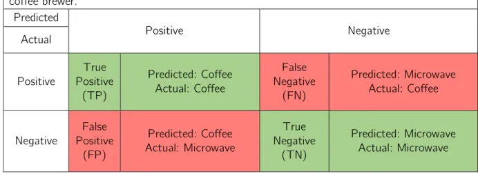
A confusion matrix is a way to visualize performance in machine learning classification. It is used to show how accurate an algorithm is in determining the different classes [32]. Below in table 3 is an example of how to think when reading a confusion matrix. True Positive (TP): The predicted value is true, and the actual value is true. False Positive (FP): The predicted value is true, and the actual value is false.

(28)

21

True Negative (TN): The predicted value is false, and the actual value is false. False Negative: (FN): The predicted value is false, and the actual value is true.

Table 3: Shows an example of a confusion matrix for the different possible outcomes of a coffee brewer. Predicted Positive Negative Actual Positive True Positive (TP) Predicted: Coffee Actual: Coffee False Negative (FN) Predicted: Microwave Actual: Coffee Negative False Positive (FP) Predicted: Coffee Actual: Microwave True Negative (TN) Predicted: Microwave Actual: Microwave

2.9.2 Accuracy

Accuracy is the most intuitive measurement; it simply measures “how accurately did we classify the different classes?”. The closer the value is to 1, the higher the accuracy has been achieved. If there is a high-class imbalance in the data set accuracy is not a good measurement [33].

𝑇𝑃 + 𝑇𝑁 𝑇𝑃 + 𝑇𝑁 + 𝐹𝑃 + 𝐹𝑁

2.9.3 Cross-validation

Cross-validation is a way of measuring accuracy and decreasing the risk of overfitting the algorithm when there is a low amount of data. Overfitting is the case when the algorithm learns the details in the training data too well which negatively impacts the algorithm on new, unseen, data.

There are different kinds of validation but in this thesis, we have used K-fold cross-validation which works by splitting the data set into K-amount of smaller pieces, called folds, and the measurement runs K-amount of times where each time it uses a different fold as the test set and the rest as the training set. The average score is then calculated to get the effectiveness [26] [34]. The K value for this thesis was set to 5 which equals to each fold representing 20% of the total data. Below in table 4, there is an example of how cross-validation works.

(29)

22

Table 4: An example table to show how cross-validation works. In this example K=3. FULL FEATURE DATA SET

Test data Train data

Fold-1 Fold-2 Fold-3

Split-1 Test Train Train

Split-2 Train Test Train

Split-3 Train Train Test

2.9.4 Precision

Precision is the algorithms ability to correctly label predicted positives, that is how many of the predicted coffee brewers were actual coffee brewers. i.e. How many of the classes it thought were coffee brewers were actual coffee brewers? If the algorithm would label 100% of the predicted coffee brewers correct, the result would be 1. The higher the value, the lower the false positives is in the classification, which is the wanted result [35].

𝑇𝑃 𝑇𝑃 + 𝐹𝑃

2.9.5 Recall

Recall, or sensitivity, is the algorithms ability to label actual positives, that is how many of the actual amounts of coffee brewers were correctly predicted. i.e. How many of our coffee brewers did it classify as coffee brewers? If the algorithm would label 100% of the actual coffee brewers correct, the recall result would be 1 [35].

𝑇𝑃 𝑇𝑃 + 𝐹𝑁

2.9.6 F1-score

F1-score is the weighted average between precision and recall. Which means that it takes both False Positives and False Negatives into account, this is very useful when the data has an uneven class distribution [36]. A good F1-score means that the classification has achieved a low number of False Positives and False Negatives which means that the higher result achieved, the lower amount of untrue values is in the result [35].

2 × 𝑝𝑟𝑒𝑐𝑖𝑠𝑖𝑜𝑛 × 𝑟𝑒𝑐𝑎𝑙𝑙 𝑝𝑟𝑒𝑐𝑖𝑠𝑖𝑜𝑛 + 𝑟𝑒𝑐𝑎𝑙𝑙

(30)

23

3 Result

The low-cost prototype system resulted in a total cost of 721SEK or 77,59USD. Our findings from the theoretical classification show that Random Forest from Group-A is the best performing algorithm with a cross-validation accuracy of 94,4% and an F1-score of 93,4%. This makes it the best-suited algorithm for this kind of machine learning

classification with the features of maximum value, minimum value, mean value, and standard deviation when the sliding window size is 1000 data points. Table 5 shows the difference in accuracy between the different machine learning algorithms.

For our recurrent neural network LSTM in Group-B, the result was 25,8%. No F1-score was measured for the LSTM algorithm, therefore, it is not present in table 5 below.

Table 5: Shows the cross-validation accuracy and the F1-score achieved for the different machine learning algorithms.

Algorithm Cross-validation accuracy F1-score

K-NN 90,8 % 93,0 %

RF 94,4 % 93,4 %

DTC 91,8 % 89,8 %

LSTM 25,8 % -

3.1.1 Confusion matrix

In this section, there is a confusion matrix for each of the algorithm in Group-A. The matrices show one of the splits during our cross-validation. The matrices also show how many devices of each class the algorithm got correct and if it didn’t classify it correct it shows what it was classified as instead. This provides a good overview of how many of each appliance was tested, what devices were similar and the basic results. Note that the confusion matrices 1, 2 and 3 do not represent the exact score presented in this thesis since the accuracy score is an average of five folds for each algorithm.

3.1.1.1 k-Nearest Neighbors result

k-NN had a cross-validation accuracy of 90.8% and an F1-score of 93.0%.

Confusion matrix 1: Shows a confusion matrix for the k-NN algorithm.

Predicted coffee dishwasher fridge micro toaster vacuum All Actual coffee 4 0 0 1 0 0 5 dishwasher 0 8 2 0 0 0 10 fridge 0 0 14 0 0 0 14 micro 0 0 0 7 0 0 7 toaster 0 0 0 0 5 1 6 vacuum 1 1 0 0 0 2 4 All 5 9 16 8 5 3 46

(31)

24

3.1.1.2 Random Forest result

RF had a cross-validation accuracy of 94.4% and an F1-score of 93.4%.

Confusion matrix 2: Shows a confusion matrix for the RF algorithm.

3.1.1.3 Decision Tree Classifier result

Decision Tree Classifier had a cross-validation accuracy of 91.8% and an F1-score of 89.8%.

Confusion matrix 3: A confusion matrix for the DTC.

(32)

25

4 Analysis

In this section, we will explain and analyze some of the decisions taken for this thesis. We have separated the analysis part into Group-A and Group-B. Then we will analyze more general topics such as the problem with measuring only current, how the selected appliances and online data sets may affect the result as well as the platform cost.

4.1 Group-A

In this section, we will analyze the sliding window and how its size was determined, the selected features and their importance for Group-A.

4.1.1 Size of the sliding window and preventing overfitting

As mentioned in section 2.5.1 Sliding window, the sliding window that extracts the important features from the data sets was set to 1000 data points when classifying appliances in real time. For the training data set the sliding window was 1000 data points for all appliances except for fridge and dishwasher where it was 6000. The reason for having the sliding window six times larger for these two particular appliances was to prevent overfitting of the algorithms. Overfitting is the case when the algorithm models the training data too well [26]. The algorithm that is trained could then give a very high accuracy when testing against the test data if it is very similar to the training data, but it may not perform as well against unseen data, in our case, that means when classifying unseen appliances in real time.

This overfitting is highly likely in our own collected data if we have a too small sliding window. For example, a fridge might have a startup period of about 100 data points (2 seconds) before it reaches its steady state as can be seen in graph 8. Then it will continue with that steady state for approximately 80.000 data points (26 minutes) as can be seen in graph 2. This means that during this long steady state the data points will barely change and therefore, as expected, it will produce very similar features for the whole load signature.

Having a lot of similar data may also result in a false accuracy since the data in both the training data set and testing data set might be very similar. This results in that the algorithm won’t be tested against unseen data. This could be avoided by either collecting more load signatures from other models of the same type of appliance to even out the data since the steady state can be different for different models.

Increasing the sliding window size proportionately for the devices with a longer load signature would also help to decrease the risk of having a class imbalance in the training data. This is why we have chosen to have a larger sliding window on the appliances which have longer load signatures. As visible in the graph 13 and graph 14, the accuracy could be interpreted as very good when the sliding window is very small for all devices, but our confusion matrices combined with inspecting the training data proved that the machine learning algorithm was overfitted and therefore the sliding window size had to be increased.

(33)

26

Graph 13: The different accuracy for cross-validation depending on window size.

Graph 14: The different F1-scores depending on the window size.

4.1.2 Sliding window size graph interpretation

The result of F1-score can change depending on which data became train or test data. The F1-score was averaged from running the machine learning algorithms five times. When calculating the Cross-validation score it was not necessary to run it multiple times since it automatically does this. This was done for each machine learning algorithm in all different sliding window sizes as seen in graph 13 and graph 14.

As visible in graph 13 and graph 14 Random Forest was the algorithm that gave the highest accuracy regardless if the sliding window size is taken into account or not. In the first two windows (100 and 250 window size) we are confident that the algorithms were overfitted.

As we moved towards a large sliding window, we noticed a steady decrease in the accuracy but also that the data showed a decreasing amount of evidence of overfitting. This was why we settled for 1000 sliding window (6000 for dishwasher and fridge) since larger sliding window removed too much data resulting in underfitting the machine learning algorithms and a smaller sliding window showed signs of overfitting.

(34)

27

We also looked at the data during the sliding windows to see if there were many instances of features that were the same or very close to having the same values, as this would result in overfitting the machine learning algorithms. This was especially true for

dishwashers and fridges; therefore, it was relatively easy to determine when the machine learning algorithm was overfitted.

4.1.3 The selected features and their importance

The features that get extracted inside the sliding window could also affect the accuracy score. In this thesis, we have chosen the following features: maximum value, minimum value, mean value, and standard deviation. All of these are relatively simple features, but as proven in section 3. Result, they still give very good accuracy. How they differ in importance for the different algorithms can be seen in table 6. k-NN doesn’t work in the way that the different features are more important than others and therefore it is not evaluated in the table.

Table 6: Shows the feature importance when using 4 features. Algorithm Maximum

value

Minimum value

Mean value Standard deviation

RF 26,3 % 12,4 % 37,6 % 23,7 %

DTC 13,6 % 7,0 % 50,7 % 28,7 %

It is clear that mean value is the most important feature for both of the algorithms. The reason for this is probably because most of our instances of features in the data are when the appliances are in their steady state. During that cycle, the features don’t differ that much in maximum or minimum value, which makes their mean value more helpful in the classification.

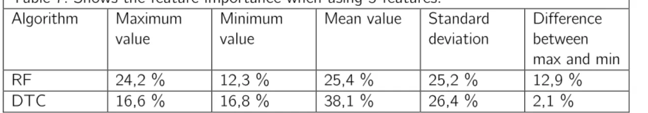
In the first stages of this thesis, we also tested to have one additional feature and that was the difference between the maximum and minimum value in each sliding window. The results from this and their importance can be seen below in table 7.

Table 7: Shows the feature importance when using 5 features. Algorithm Maximum

value

Minimum value

Mean value Standard deviation

Difference between max and min

RF 24,2 % 12,3 % 25,4 % 25,2 % 12,9 %

DTC 16,6 % 16,8 % 38,1 % 26,4 % 2,1 %

During this same testing, we also noticed that the accuracy score for the different algorithms was lower with the fifth feature added and therefore it was removed to

improve the accuracy. The accuracy score from this testing with the feature added can be seen below in table 8.

(35)

28 Table 8: Shows the accuracy when having 5 features. Algorithm Cross-validation accuracy F1 score K-NN 89 % 82 % RF 93 % 91 % DTC 90 % 80 %

4.2 Group-B

In this section, we will analyze Group-B and the effects LSTMs hyperparameters and the low amount of data could have had on the results.

4.2.1 Tuning the hyperparameters of LSTM

There is no “correct” way to tune the parameters and different layers of an LSTM algorithm. It's mostly a trial and error approach to see if the results get better or worse and work from there. This is because LSTM is highly customizable and can be used for multiple different problems.

To tune the parameters, we looked at different settings in our LSTM and changed some of those to see how much we could increase the accuracy. Below we will show different graphs and the different accuracy achieved when those parameters were changed. Each graph had the “best” settings from the other parameters.

As visible in the graphs 15-18, the accuracy barely changed with the different parameters. The reason for this is hard to say since the test with the Tracebase data, as mentioned in section 2.8.2.1 LSTM, returned an accuracy of 95,7% and that showed that the

algorithm had good parameters for our kind of approach with features and sliding windows.

When training the LSTM model on the Tracebase data set and using our own collected data for testing it returned an accuracy of 24.5%. The reason for why this accuracy is so low could be because the trained model could not generalize good enough on the

Tracebase data. It could also be because the data in the Tracebase data set is very similar to each other, and our own collected data is not similar to the Tracebase data.

4.2.1.1 Hyperparameters graphs

Below there are four different graphs showing the different tuning of the hyperparameters for the LSTM algorithm. Each graph has the best-achieved hyperparameters from the other parameter tuning results.

(36)

29

Graph 15: Accuracy for LSTM depending on the size of the sliding window.

(37)

30

Graph 17: Accuracy for the LSTM algorithm depending on sequence length.

Graph 18: Shows the accuracy depending on two different dropout parameters. The x-axis is the 2nd dropout parameter. The different colored bars represent different sizes of dropout parameter 1.

Graphs 15-18 are representations for the different hyperparameters and how the tuning affected the accuracy achieved for LSTM. For each graph, the best result from the other tests was incorporated.

Graph 15 shows the accuracies achieved for different sliding window sizes. The best-achieved accuracy of 25,72% was with a sliding window size of 100 data points which is a

(38)

31

lot smaller than what we used for Group-A where each sliding window size was 1000 data points. RNNs requires a lot more data compared to other classification algorithms so therefore a smaller sliding window for LSTM increased the amount of data and this means it could achieve higher accuracy.

Graph 16 shows how the accuracy changes depending on the number of epochs used. Each epoch size was evaluated with both the training and testing data set. As can be seen in the graph a lower number of epochs resulted in lower accuracy, but after reaching 100 epochs the accuracy didn’t change. Not visible in the graph is the loss recorded for each set, but the loss also stopped decreasing as the number of epochs was increased to 100. Graph 17 displays the non-existent changes of accuracy depending on sequence length. The accuracy always remained the same and wasn’t affected by the sequence length for the algorithm. Loss is not visible in this graph, but the loss was the smallest when the sequence length was 5, therefore we decided that the sequence size of 5 was the best for this thesis.

Graph 18 shows the accuracy depending on the two different dropout parameters. The bars display dropout parameter 1. The x-axis displays dropout parameter 2. As can be seen in the graph having a second dropout parameter as either 0,1 or 0,2 doesn’t change the accuracy but as soon as the dropout parameter 2 increased, the accuracy went down fast. Therefore, we chose to have a dropout parameter 2 as 0,1 and dropout parameter 1 as 0,4.

4.2.2 Low amount of data

Recurrent neural networks usually require a high amount of data [29], something that we don’t have. As shown in section 2.8.2.1 LSTM, we used a different data set called Tracebase to test our LSTM model. Tracebase had a lot more data per device compared to what we were able to collect on our own. When using the Tracebase data set we used the same type of features and sliding window approach as we did for our own data set and was able to achieve a much higher accuracy (95,7%) compared to our own collected data (25,8%).

The reason for not using this data set in our real world testing as training data was that Tracebase contains data from 1Hz (1 second) to 0,125Hz (8 seconds) with no clear pattern between the different measurements, and therefore it would not be representable as data for us as we were measuring data at a rate of 50Hz. We wanted our prototype to quickly be able to classify devices in real time and using Tracebase would not be

representable of “quickly” since sometimes the data points would have too long of a time span between them.

4.3 The problem with only measuring current

As mentioned earlier, in the original NILM, both the current and voltage gets measured at a single sensing point. In this thesis we chose to only measure current to keep the cost of the prototype system low and also because measuring both current and voltage have previously been done [7] and therefore, we wanted to see how good accuracy we could achieve if we only measured the apparent power.

(39)

32

EmonLib can be used for more than just measuring apparent power as we do in this thesis. For example, if you also would use an AC to AC power adapter that measures voltage together with the CT-sensor it would be possible to acquire information about real power, apparent power, power factor, RMS voltage, and RMS current.

As can be seen in section 3.1.1 Confusion matrix there are some instances of appliances that gets repeatedly classified as the wrong appliances. For example, some of the

instances of features from the dishwasher appliance category get classified as not being a dishwasher in all three chosen algorithms. If we examine these extracted features data, more closely it looks like this:

It is clear that these two instances of data are very similar to each other, even though they are from two different appliance categories. This is because the dishwasher has a cycle in its load signature that is very similar to a cycle from one of the fridges. This is a great example of where our prototype system has its limitation in the way that we only collect current and therefore don’t acquire enough detailed data that could have differentiated these two appliances apart. In this particular case of the wrong classification, it probably could have been resolved by also collecting voltage. This is because fridges contain capacitance components and which mean its reactive power might have looked different than a dishwashers reactive power and therefore could have helped in the correct classification [6].

4.4 Selected appliances

The appliances that were selected for evaluating the different algorithms could drastically change how good of an accuracy score that was achieved. Ideally, all different kinds of appliances in a home would be evaluated although this would have been very

time-consuming. The results we achieved could also be affected by the appliances we chose for this prototype. The reason for selecting the different types of appliances was to make the classification more complex and real-world. However, the results we achieved might still not represent a correct score if the proposed prototype would be expanded with more devices. For example, in the prototype, the dishwasher was falsely classified as a fridge with all three different machine learning algorithms in Group-A. This lowered the overall accuracy score of the algorithms. In a real-world scenario, there might be appliances that are more similar to each other than in our prototype and this could lower the accuracy score.

4.5 Online data sets

The large online data sets lack details such as sometimes not even measuring one value each second, meanwhile the small data set lacks concurrent devices, and also had too slow of a data collection rate, therefore this was not an option. If we would have used a large data set, we would have gotten a lot of devices but with much less detailed data. class,maximum,minimum,mean,standard_deviation

dishwasher, 115.73,102.1,108.26,1.68 fridge, 115.22,99.13,108.09,4.72

An approach to evaluate machine learning algorithms for appliance classification