The Effects of Capital Income Taxation on Consumption : Panel data analysis of the OECD countries

The Effects of Capital

Income Taxation on

Consumption

BACHELOR

THESIS WITHIN: Economics NUMBER OF CREDITS: 15

PROGRAMME OF STUDY: Civilekonom

AUTHOR: Arvid Aronsson and Daniel Falkenström JÖNKÖPING May 2021

Bachelor Thesis in Economics

Title: The Effects of Capital Income Taxation on Consumption Authors: Arvid Aronsson and Daniel Falkenström

Tutor: Johannes Hagen

Date: May 2021

Key terms: Dividend Income, Private Consumption, Panel Study, Capital Income Taxation, Tax planning, OECD

Abstract

This thesis investigates if the tax rate on dividend income has a significant effect on private consumption expenditure. This is done through a panel study on 36 OECD countries during the period 2000-2019. Regressions using differenced data and several control variables are used. The results are to some extent in line with previous empirical work studying the effects of tax changes on consumption. The results indicate that the taxation of capital income in the form of the overall tax rate on dividend income does not have a significant effect on private consumption expenditure. The theoretical mechanism deemed most likely to be in effect is tax planning since contradictory results are obtained regarding the effects of other tax rates in the form of taxes on labour income and VAT on private consumption expenditure.

Table of Contents

1.

Introduction ... 1

1.1 Purpose ... 2

1.2 Limitations ... 3

2.

Theory and Literature Review ... 4

2.1 Fundamentals of Consumption Theory ... 4

2.1.1 Keynes’ early theory and the Marginal Propensity to Consume ... 4

2.1.2 A Modern Theoretical Consumption Function ... 4

2.1.3 The Income Effect and the role of Taxes in consumption theory ... 5

2.2 Mechanisms to explain why Taxes do or do not affect Consumption Behavior ... 5

2.2.1 Ricardian Equivalence ... 5

2.2.2 The Permanent Income Hypothesis and Consumption Smoothing ... 6

2.2.3 Tax Planning and Competition ... 7

3.

Hypothesis ... 9

4.

Institutional Background ... 10

5.

Empirical Methodology ... 12

5.1 Data sources and scope ... 12

5.2 Dependent Variable ... 12

5.3 Explanatory Variables ... 12

5.4 Expected Signs ... 15

5.5 Descriptive Statistics ... 16

5.6 Tests for determining econometric models and specifications ... 19

6.

Econometric Model and Empirical Results ... 22

6.1 Econometric Models ... 22

6.2 Empirical Results ... 24

6.3 Robustness Tests ... 26

7.

Analysis and Discussion of the Results... 29

8.

Conclusions ... 32

Reference list ... 33

Figures

Figure 1: PCPC Descriptive Statistics... 16

Figure 2: ΔPCPC Descriptive Statistics ... 17

Figure 3: CITR Descriptive Statistics ... 18

Figure 4: ΔCITR Descriptive Statistics ... 18

Figure 5: Graphical test for Heteroscedasticity ... 28

Tables

Table 2: Descriptive Statistics ... 16

Table 3: Results of Individual Root – Fisher – ADF tests ... 20

Table 4: Results of Panel Cointegration tests ... 21

Table 5: Sequential Pooled OLS results ... 22

Table 6: REM and FEM testing ... 24

Table 7: Regression results ... 25

Table 8: Correlation Matrix ... 26

Table 9: Variance Inflation Factors ... 26

Table 10: Autocorrelation Corrected FEM Regression Output ... 27

Equations

Equation 2: Disposable Income ... 5

Equation 3: Pooled OLS ... 22

Equation 4: REM Regression ... 24

Appendix

Appendix 2: Individual Country Regressions ... 36

Appendix 3: Unit-root tests ... 37

Appendix 4: Cointegration Tests ... 42

Appendix 5: Regressions output ... 43

Appendix 6: REM and FEM testing ... 48

1. Introduction

Private consumption expenditure is typically the largest component of the classical GDP-equation in macroeconomic theory. Indeed, it has been observed to make up 50-60% of GDP in most countries (Gottfries, 2013). Policies that could influence consumption can therefore have large effects on the economy as a whole. It is therefore interesting and useful to know what affects consumption expenditure and how it is affected.

Among the most used and discussed policies is tax policy, as changes in tax rates and rules can significantly change incentives and abilities for consumers and firms as to how they deploy and allocate their resources. A higher tax rate on different kinds of income should in theory reduce disposable income and thus also consumption expenditure.

Dividend income and capital gains from assets are examples of capital-related income to households that could be used for consumption. Notably, this type of income can be of large quantity and its share of total income has substantially grown over recent years (Roine & Waldenström, 2012). Though also, the distribution of this particular type of income is significantly skewed towards wealthier and higher-income individuals and households (Roine & Waldenström, 2012). Both from the perspective of economic efficiency and in the interest of responding to growing income and wealth inequality, the taxation of capital income has lately become of greater interest for economists and policymakers (Waldenström et al., 2018). Taxing capital can be a large source of income for the government and could be used to redistribute wealth from richer to poorer individuals and groups if that is deemed an objective.

However, what other effects could the taxation of capital income have on the economy and the incentives of economic actors? For example, it has long been reasoned that taxing the income and profits of corporations could incentivize them move their operations to other countries, so the government then misses out on that taxable income. Alternatively, profits and dividends could be kept unrealized in order to not pay taxes on them. Most relevant for this study, does higher capital income taxation decrease private consumption expenditure through the income effect or is capital income not a base for consumption expenditure to the extent that labor income is?

Much research has been done on the effects of income taxation on consumption expenditure. Empirical studies like Haug (2020) conclude that tax changes significantly affect consumption expenditure. Several studies have also been made on for example specific tax cuts, like the Reagan tax cuts which shows that tax rebates do have significant effects on consumption (Souleles, 2002). One advantage of such reform-based studies is that the amount and timing of tax rebates and thus disposable income changes is known and that the specific cause and effect can more easily be identified. Different groups can be affected differently, and you can therefore study causal effects. Furthermore, the previously mentioned study also indicates that the marginal propensity to consume from this increased disposable income differs for different income groups (Souleles, 2002).

In contrast, there is a lack of research on the effects of capital taxation on consumption. One potential reason for this is the absence of clear capital income tax reforms. We contribute to this literature by studying the effect of a capital tax rate in the form of the overall dividend income tax rate on consumption in the OECD countries. We also want to compare the effects of capital income taxation to that of labour income and consumption taxes in the form of VAT. This study could be of value because awareness of these effects are vital when pursuing efficient tax policy. Additionally, the consumption changes in particular should be seen as important because of consumption expenditures large share of GDP thus its effects on the economy.

1.1 Purpose

The purpose of this thesis is to investigate if the taxation and tax rates on capital income affects households’ consumption expenditure in the OECD countries during the period 2000-2019. More specifically we focus on the combined effect of the tax rate on corporate income plus the tax rate on the dividend income to capital owners. This rate gives a comparable number for the general level of taxation of dividend capital income. The goal is to see if higher or lower tax rates on capital income changes households’ level of consumption and if changes in the tax rate on capital income significantly affects consumption expenditure at an aggregate level. Formally stated, the purpose is to answer the following research question:

Does the overall corporate income tax rate plus private dividend tax rate significantly affect aggregate consumption expenditure in the OECD countries during the period 2000-2019?

1.2 Limitations

With our choice of data and scope, examining only the dividend income tax rate and not the tax rate on capital gains, there are several limitations that follow. One limitation of our study is that we only look at the dividend income tax rate and not at the capital gains tax rate. This means that one could potentially directly neglect a large share of the capital income that is earned and thereby that this scope fails to recognize important effects.

One major problem with modelling economic data is that it is difficult to control for enough relevant variables, without running into problems such as multicollinearity. In the model, the dependent variable is private consumption per capita, however this fails to account for how far the social insurance provided by governments extends. What this means is that we may very well have significantly different levels of autonomous consumption across the different countries, this can however be partly controlled for by using country-specific effects in the panel data regression.

Increases in the debt level in countries are in this thesis not included as a control variable, despite that this may very well have a significant effect on private consumption expenditure. This omission of a potentially important control variable opens up for questions, if debt were to be incorporated into the model, it could cast doubt on the results or reinforce them.

In chapter 2, several different theories which can explain or partly explain different economic behaviors are presented. Identifying which one of them is actually in effect will be difficult to distinguish, however it is not the primary purpose of this thesis to do so.

Finally, another limitation is that by only analyzing a period of 20 years, the results should perhaps be viewed as sample results and not population results because of some potential factors specific to this period. This means that the results may not be suitable to generalize for other time periods.

2. Theory and Literature Review

In this chapter we will summarize the theoretical framework and various empirical contributions related to our study.

2.1 Fundamentals of Consumption Theory

To understand and study how changes in an income tax rate affects consumption expenditure we begin by describing the classical economic theory of what determines and affects consumption expenditure. Thus, we will start by briefly reviewing the fundamentals of consumption theory.

2.1.1 Keynes’ early theory and the Marginal Propensity to Consume

According to Keynes (1936), ”the amount of aggregate consumption mainly depends on the amount of aggregate income”. Thus, Keynes is known for the consumption function which is dependent mainly on aggregate income. Income positively affects consumption expenditure so that they increase together. However, note that Keynes also identified other motives for why individuals would refrain from consuming. Among these are the future assurance of well-being and thereby the need of reserve funds, low expected future income due to old age and inability to work or the possibility to earn interest and/or appreciation to in the future consume more than today (Keynes, 1936).

Central to Keynes’ theory of consumption is also the concept of the marginal propensity to consume. As stated, consumption is a positive function of aggregate income. The extent to which an increase in income increases consumption, or the share of additional income that is consumed is the marginal propensity to consume out of income. This share is lower than one according to Keynes (1936) who thereby posits that people do not consume all the additional income they receive. Furthermore, as has been empirically observed by Fisher et al. (2020) the marginal propensity to consume is generally lower for wealthier individuals than for poorer individuals.

2.1.2 A Modern Theoretical Consumption Function

Keynes fundamental theory of what determines consumption is still the basis for modern consumption theory and functions. However, we will now give a more modern example of a textbook consumption function depending on more variables than just income.

Gottfries (2013) specifies a consumption function relating consumption to four factors:

Equation 1: Gottfries (2013) Consumption Function

𝐶 = 𝐶(𝑌, 𝑌𝑒, 𝑟, 𝐴)

These four factors, Y,Ye, r, A, are income, expected future income, the real interest rate and assets, respectively. Y,Ye and A all positively affect consumption as they all make up the base to be used for consumption. However, the real interest rate, r, negatively affects consumption as it makes saving more attractive and borrowing more costly.

2.1.3 The Income Effect and the role of Taxes in consumption theory

If we view the income variable in the above consumption function as the disposable income after paying taxes on the gross income, it is evident that taxes on income negatively affects consumption expenditure. If the tax rate is τ (which could be both a labour income tax rate or a capital income tax rate), the disposable income, 𝑌𝐷, is calculated as such:

Equation 2: Disposable Income

𝑌𝐷 _{= 𝑌}𝐺_{(1 − 𝜏) + 𝑇𝑟}

Where 𝑌𝐺 _{is the gross income and Tr is transfers. A higher income tax rate decreases} disposable income. This is to say, taxes negatively affect consumption through the income effect. When households are taxed, their disposable income decreases and so then does their ability to consume.

2.2 Mechanisms to explain why Taxes do or do not affect Consumption Behavior

After briefly reviewing the classical theoretical framework of the consumption function we will now discuss and review further theories of consumption and taxes. The theory in the previous section mainly points to there being a relationship between income tax rates and consumption expenditure that is negative. However, further theories and empirical studies can give more arguments both for and against that theoretical relationship.

2.2.1 Ricardian Equivalence

Ricardian equivalence, famously developed by David Ricardo in 1820 and Barro (1974), is a theory that assumes consumers are forward looking and will realize that if taxes are lowered now, while government spending is not reduced, taxes will need to be raised in the future (Ricciuti, 2003). That means they cannot use the increase in income from the tax reduction for consumption since it has to be saved for when taxes are again raised. As

such, this is one theoretical mechanism that points toward tax rate changes not affecting consumption expenditure.

Haug (2020) empirically examines the Ricardian equivalence hypothesis using economic data and concludes that it does not hold. Tax rate changes were found to have a significant effect on consumption expenditure even when spending was unchanged. Furthermore, Hayo & Neumeier (2017) investigates if Ricardian equivalence holds in reality by method of a survey on the German population regarding deficits, taxes and consumption behavior. They conclude that “RET has little practical relevance for people’s economic behavior” because the majority of the survey respondents did not act in a Ricardian manner in response to larger deficits. Poterba (1988) in studying two temporary income tax changes in the 1960’s and 1970’s found that consumers were more responsive to tax changes than anticipated by theory. Notably Poterba also found that “the timing of taxes appears to affect the level of real activity” which again speaks against Ricardian equivalence. Poterba also sheds light on the fact that there are several important factors besides what is mentioned above. Such as imperfect financial markets and households with liquidity constraints, decreasing their ability to follow what theory predicts. In summary, much of the empirical work speaks against Ricardian equivalence theory.

2.2.2 The Permanent Income Hypothesis and Consumption Smoothing

Friedman (1957) in his seminal book “A theory of the consumption function” points out the distinction between what he calls peoples’ temporary income and their permanent income for consumption theory. This theory has since been called the Permanent Income Hypothesis (PIH) and says that consumption behavior will only be changed in response to changes in consumers’ permanent income, not their temporary income. As such, consumers are assumed to be forward looking and to take into account expected future income. For example, tax reductions today may be seen as temporary and people will therefore not increase their consumption. Consumption will increase only if consumers believe taxes have been permanently reduced (Gottfries, 2013).

Empirical results regarding the PIH are mixed. From the previous section, Poterba (1988) found that consumers responded to temporary income tax changes. Additionally, Souleles (1999) studied the consumer response to a specific type of income increase that is transitory in nature: income tax refunds. Souleles found that the consumption response to the tax refunds exhibited enough excess sensitivity to reject the permanent income

hypothesis. Furthermore, liquidity constraints were again found to be an important factor. The liquidity constraints issue falls in line with the observation of a relatively higher MPC for low-income households. Souleles (2002) has a very similar conclusion in studying the consumer response to the Reagan tax cuts, as excess sensitivity is again found of an even larger magnitude. Also, since the income was predictable, the PIH is again not supported. Souleles also explicitly states that the explanation for the result is unclear. Caroll (1997) argues that the PIH is not empirically supported because consumption behavior is better described by a “Buffer-Stock” theory. This theory assumes the growth in average consumption expenditure follows the growth in average labour income and is consistent with the higher MPC empirically observed according to Caroll.

2.2.3 Tax Planning and Competition

Taxes may affect consumption, taxes may affect disposable income, but tax policy may also affect companies’ strategies. In a cross-country setting, the most basic ideas about competition can be applied in the sense that if one country reduces their taxation levels, the neighboring countries may mimic this to not lose taxable income streams and capital stock. The tax competition theory has been tested empirically, for example by Chirinko & Wilson (2017) who tested the capital taxation among U.S states in a panel setting. They found that the reaction function was negative, which means that tax competition in this setting is not a race to the bottom. That is if one country decreases its capital tax rate, the other follows. But there is also evidence that countries do race to the bottom by successively introducing a lower corporate income tax than their neighboring countries (De Mooji & Nicodéme, 2006). One possible implication of this is that there could be a general trend over time where capital income tax rates decline in many countries. Indeed, the capital income tax rate has been lowered in many developed countries in recent years (Chirinko & Wilson, 2017). Another possible implication of international capital tax competition is that capital income tax rates will not affect consumption because corporations and people move capital so as to pay taxes in a different country in response to a higher tax rate in the original country. That is one possible mechanism to explain a scenario where capital income tax rates do not affect consumption.

With larger multinational corporations there are further elements to consider than the legislators view discussed briefly above. Multinational entities have the possibilities to shift their profit to different jurisdictions if the tax incentives are large enough. That is, if

the tax benefits are greater than the shifting costs firms could be inclined to shift entire production lines. This may work as bargaining power for corporations when negotiating with labour unions regarding wages. If a country has a lower corporate income tax rate it is possible to remain attractive for firms even if it were to have a high average wage level. The tax pressure in combination with the national average wage level affects companies’ profits and thereby their decision of where to locate (Krautheim & Schimdt-Eisenlohr, 2016). The above discussion indicates that a multiplex relationship could exist between variables of taxes, wages and thereby consumption expenditure.

When tax rates change, owners can alter the label of the income they receive, for example to avoid having to pay an increased tax rate. This is called income shifting. Empirically this has been observed to be the case. When the 2006 Swedish dividend tax rate was decreased, there was a significant shift in income from wages to dividend income. This was most pronounced for managers who also were the owners of the firms. The dividend income was increased but the overall income was unchanged implying that this is simply a form of tax planning (Alstadsæter & Jacob, 2016). This kind of behavior is another possible mechanism to explain a finding that tax rates on dividend income do not affect consumption expenditure. If the tax rate is changed but the same amount of income is still taken out under a different label, consumption expenditure would not be affected through the income effect.

3. Hypothesis

Traditional economic theory would suggest that if capital dividend income is a significant part of peoples’ income, the tax rates on it should affect aggregate consumption expenditure. It can be argued that higher tax rates should lead to lower consumption expenditure simply because of the income effect. However, many alternative and complimentary theories like Ricardian Equivalence and the Permanent Income Hypothesis as well as strategies of tax planning provide a theoretical foundation for the argument that changes in the tax rates on capital will not affect consumption expenditure. These classical theories are often referred to in the context of labor income and may or may not apply to the same degree in the context of capital income, specifically dividend income. Furthermore, it has been empirically observed that capital income is skewed towards accruing to wealthier individuals and households (Roine & Waldenström, 2012). Together with the fact that wealthier individuals have a relatively lower marginal propensity to consume (Fisher et al., 2020), it could also be theorized from a “Keynesian” perspective that capital income taxation will have a weaker effect on consumption expenditure than other forms of taxation such as labor income taxation. However, this particular explanation could be difficult to argue for in an empirical context because labor income is already a much larger share of total income than capital income (OECD, 2015).

On the other hand, much of the earlier empirical studies on tax changes effects on consumption mainly points to a stronger consumer response than suggested by theory. Though again, those studies do not mainly look at capital income and because of that our hypothesis is not swayed towards thinking we will find a large effect from capital income specifically. In summary of these factors, our hypotheses are the following:

Hypothesis 1: The tax rate on dividend capital income will not have a significant effect on aggregate consumption expenditure.

Hypothesis 2: The tax rates on dividend capital income, labor income and consumption should have a negative effect on aggregate consumption expenditure, though not all necessarily significant.

Hypothesis 3: The tax rate on dividend capital income has a weaker effect on aggregate consumption expenditure than the tax rate on labor income and the VAT rate.

4. Institutional Background

Before we get to our empirical study of our hypotheses, we will give a brief overview of some of the most important background for understanding the most important variables we investigate.

Private consumption expenditure is the market value of all goods and services purchased by households (World Bank national accounts data, 2021). It includes purchases of durable products such as computers but not purchases of property like for example houses. One very noteworthy factor related to measuring consumption expenditure in a multiple country setting like ours is that because countries have different public expenditure and social insurance systems, what is included in consumption expenditure can sometimes vary between countries. For example, in some countries’ healthcare costs may be paid for by the government but in others it may be paid for by the consumer and thus included in private consumption expenditure. This is a limitation of the study but may be partly remedied by country-specific effects.

The purposes of taxation are primarily two things, the allocation of resources to finance public functions needed in society and to discourage certain activities. Regarding the taxation of capital income in the OECD countries, there are different rules and regulations in every country. Therefore, a legal description of how taxation works cannot be given for a group of countries like the one we examine, and we will not describe any particular country’s system. We will however give a brief overview of what the capital income tax rate variable measures and how it should be interpreted.

Firstly, capital income is income derived from the ownership of different types of assets. For this thesis, we focus only on income derived from the ownership of stocks in companies. In this context, income can primarily be earned from capital in two ways. The first is through dividends, which are the shareholders’ share of the company’s profit which is sometimes paid out. The second way is through capital gains, which is when a financial asset increases in value from when the individual acquired it. Across countries there are problems with a lack of uniformity when trying to compare tax rates between countries (Waldenström et al., 2018). This problem also exists within countries, for example when differences in taxation and rates can be derived from how long an asset

has been held before the capital gain is realized, in what kind of account it is placed etc. Dividend income taxation does not suffer from this problem to the same extent as capital gains taxation does. Further, capital gains can be chosen to be or not to be realized, this being affected by numerous things, many of which is difficult to control for. For these reasons, we have in this thesis decided to only look at the dividend income tax rates.

The Organization for Economic Co-operation and Development (OECD) currently consists of 37 countries. The OECD is an international organization which works toward improving co-operation between its members in order to create solutions to economic issues. Members of the OECD must adhere to certain requirements, primarily regarding being democratic, being open free market economies and adhering to human rights. As such, the OECD countries are at least in some basic respects homogenous.

5. Empirical Methodology

This section will describe the data and method which we use to test our hypotheses.

5.1 Data sources and scope

To investigate the effects of dividend capital income tax rates on private consumption expenditure in the OECD countries we collect annual data from 36 countries in the period 2000–2019. This results in a maximum of 720 observations, however data on some variables are sometimes missing in certain years in certain countries so the effective sample size is smaller in the final model. The 36 countries included are the OECD member countries. Note that there are currently 37 members in the OECD but we do not include Columbia which joined in the year 2020 and is generally missing many data series. All data series have been collected from OECD’s or The World Bank’s databases.

5.2 Dependent Variable

In analyzing effects on consumption expenditure in a panel data setting we need a variable that describes the level of consumption expenditure and can be compared between countries. Consumption as a share of GDP is not a suitable indicator because we found that the explanatory variables could affect GDP, which was in the denominator, more than they affect consumption. This means that variables that should positively affect consumption expenditure, the employment rate for example, have a negative effect on the “consumption as a share of GDP” variable. The variable that we use as our dependent variable is instead a version of “Private Consumption Expenditure per capita”. Specifically, the data series we use is “Households and NPISHs Final consumption expenditure per capita (constant 2010 US$)” from the World Bank national accounts data. It measures the market value of all goods and services purchased by households, including durable products such as computers but not purchases of dwellings (World Bank, 2021). It also includes the expenditures of non-profit institutions serving households (NPISHs). Additionally, the data are in constant 2010 U.S. dollars, which helps measure the true or real changes in consumption expenditure adjusting for price changes. The variable will henceforth be abbreviated as PCPC for Personal Consumption Per Capita.

5.3 Explanatory Variables

The main variable of interest for this study is the overall rate of taxation of dividend capital income. The subject of capital income taxation is complex, with different rules, rates and brackets among different income types. However, the focus of this thesis is on capital income in the form of dividends to capital owners. For most countries, this type of income is first subject to the Corporate Income Tax (CIT) rate on the corporation’s profit and then a Personal Income Tax (PIT) rate on top of that paid by the dividend recipient. Various types of reliefs and credits that sometimes apply to combat double taxation is also taken into account in this indicator (OECD, 2021). The combined effect of these two tax rates gives a picture of the overall rate of taxation on dividend income. It is this indicator that is our main explanatory variable. Specifically, the data series we use is “Overall PIT + CIT rate” from the OECD Tax Database table on Overall statutory tax rates on dividend income (OECD, 2021). The variable will henceforth be abbreviated as CITR for Capital Income Tax Rate.

Top marginal personal income tax rate for employees

The personal income tax rate on labor income is the tax rate that employees pay on the wage they receive from working. Labor income taxation is also a complex subject and consists of non-uniform tax rates depending on the level of income. For our variable we look at the top marginal personal income tax rate at the earnings threshold where this rate first applies. Furthermore, this is the combined personal income tax rate accruing to the central and sub-central government. “Top marginal rate” means that the rate is calculated as the additional tax resulting from a unit increase in gross wage earnings. Note also that this rate is for the top bracket of wage earners. The data series is collected from the OECD tax database. This can be somewhat misleading if low wage earners pay a very different rate and if that group is better representing the country’s wage earners. Labor income to employees from working is the main source of income for the average individual. It is interesting to include in our model and compare its effect on consumption expenditure to the capital income tax rate. The variable will henceforth be abbreviated as PITR for Personal Income Tax Rate.

Value Added Tax (VAT) rate

A Value Added Tax (VAT) is a tax that is added to the price of a product sold for consumption. In that way, it is a tax on consumption which in the end is paid by the consumer (European Commission, 2021). A country may have different VAT rates on

different types of products. The rate we use is each country’s standard VAT rate from the OECD tax database. This rate is also interesting to include in our model to compare its effect on consumption expenditure to the capital income tax rate. The variable will henceforth be abbreviated as VATR for Value Added Tax Rate.

Average Wage in US dollars based on Purchasing Power Parities

The average wage expressed in the same currency (US dollars) and adjusted for prices to reflect the true purchasing power of it for all countries is included in our model. Since wages are the average individual’s main source of income this variable explains a large part of the level of consumption per capita in a country. For this reason, this is a variable we choose to control for when using consumption per capita as our dependent variable. It also heavily relates to the theoretical consumption function as a large part of the income variable. The variable will henceforth be abbreviated as AVGW for Average Wage.

The Employment rate

The employment rate is the percentage of the working age population that are currently employed. To count as employed you have to have worked at least one hour the previous week, or had a job but were absent. The working age population are people aged 15 to 64 according to OECD data, which is the data series we use. The employment rate directly is not traditionally part of a theoretical consumption function, but we deem it important to control for in our model. Employment rates are sensitive to business cycles which should affect consumption. Thus, it could serve as a proxy variable for the business cycle. It could also serve as a bit of a proxy variable for part of the expected income variable. The variable will henceforth be abbreviated as EMPR for Employment Rate.

The long-term interest rate

The long-term interest rate is the interest rate to be paid on government bonds maturing in 10 years. The data series we use is from OECD data and is calculated as the averages of daily rates. The way we want to use the interest rate variable is in terms of “the cost of loans”. However, that is not specifically what these rates indicate, though it should be closely related. The interest rate or the real interest rate is typically part of a theoretical consumption function. Loans can be used to finance consumption and investment and the long-term interest rate can indicate the price of loans. This is also a controlled variable

and will not be analyzed by itself. The variable will henceforth be abbreviated as LTIR for Long Term Interest Rate.

Dummy Variable for the 2008-2009 Financial Crisis

To be able to control for the negative effects on consumption expenditure of the 2008-2009 financial crisis, a dummy-variable which is equal to 1 only for the years 2008 and 2009 is generated. This will allow for a different intercept for the years 2008-2009. We want to control for this because the negative effects of the financial crisis are not otherwise explained in our model and could thus bias the other coefficient estimates. The variable will henceforth be abbreviated as DUMMYFC for Dummy Financial Crisis.

5.4 Expected Signs

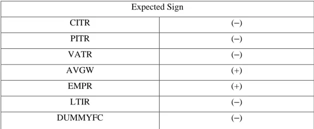
Table 1 below shows the expected signs of each coefficient in a regression model.

Table 1: Expected Signs

Expected Sign CITR (–) PITR (–) VATR (–) AVGW (+) EMPR (+) LTIR (–) DUMMYFC (–)

The expected signs above are all based on classical economic theory. Higher average wages and higher employment rates should both increase aggregate consumption. The long-term interest rate should act as an indication of the cost of loans and thus negatively affect consumption expenditure as argued in typical consumption functions. Tax rates on both labor income and capital income should both decrease consumption expenditure through the income effect as argued in the theoretical section. The variable DUMMYFC, which generates an individual intercept for the years 2008-2009 in order to control for the financial crisis, is expected to have a negative sign. The tax rate on capital income is however the most questionable in its expected sign and significance, as it is the purpose of this study. That will be the coefficient to thoroughly analyze in the results. The other

variables are control variables, and should they not have the theoretically expected sign, that could be seen as an indication of misspecification of the model.

5.5 Descriptive Statistics

Table 2 below shows some descriptive statistics of the data series for the different variables. PCPC is in constant USD, AVGW in USD based on PPP and the rest are in %.

Table 2: Descriptive Statistics

PCPC CITR PITR VATR AVGW EMPR LTIR

Mean 19668.29 42.26 39.18 18.26 36322.24 66.85 4.01 Median 21666.84 43.76 43.00 20.00 35619.42 67.63 3.99 Maximum 41852.64 74.00 62.28 27.00 79038.06 86.53 22.50

Minimum 4787.75 15.00 0.00 5.00 7313.93 44.23 -0.49

Std. Dev. 9128.49 10.43 13.65 5.57 15048.02 7.37 2.78

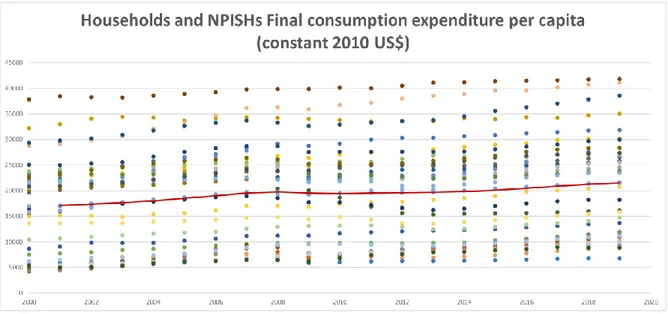
After adjusting for missing observations, the effective sample size that the statistics are based on is 672 observations. It can be seen in the table that the different data series all have a sufficient range to draw statistical inference from. The maximum values for the different variables are for the most part several times as large as their minimum values. These wide ranges are mostly explained by cross-country differences rather than changes over time. For our dependent variable private consumption per capita, this is also visualized in Figure 1 below.

In Figure 1 on the previous page, every country’s PCPC values correspond to a color and we get 36 dots for every year between 2000-2019. Figure 1 then shows how the different countries have differing levels of consumption per capita and how their rank in relation to other countries’ consumption levels change over time. While there are large cross-country differences in consumption, the cross-country rankings are relatively stable. There is a general upward trend in consumption over time. The red line shows the mean of all countries for every year and we see an upwards trend with a slight dip near the financial crisis around 2008. The changes over time are larger than it may seem in the graph, but because the vertical range is so wide changes do not seem as large. The next figure 2 addresses this by showing the change (first difference) in PCPC for every country and year.

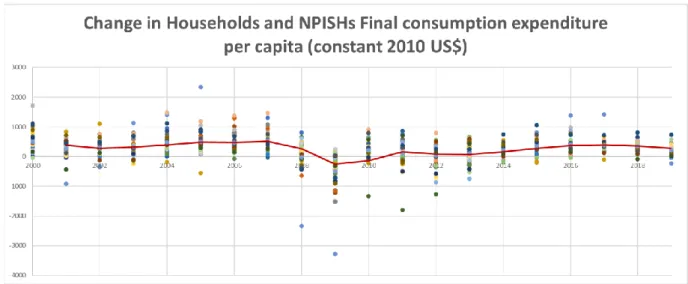
Figure 2: ΔPCPC Descriptive Statistics

The red line again shows the mean change of all countries for every year and thus shows the general trend over time. Here changes can be seen more clearly, as the mean and most of the dots are consistently above zero, meaning increases in PCPC over time, with the exception of 2009.

Figure 3 on the next page shows within- and between-country variation in capital income tax rates in the same manner as the previous graphs.

Figure 3: CITR Descriptive Statistics

Here we again see a wide range mostly explained by cross-country differences. However, there are more changes over time for this variable in terms of countries switching order and sometimes changing more drastically from one year to the next. The mean trend line shows a bit of a decrease over the years 2000-2020.

In figure 4 on the previous page, we see the annual changes in our capital income tax rate for every country. The range is again wide, but this time because we see some big outliers corresponding to large changes in the tax rates or tax reforms. On average however, the mean change is generally close the zero for most years.

5.6 Tests for determining econometric models and specifications

This section contains results of tests used to determine the suitable models and specifications for regressions on our data. The descriptive statistics visualized in the previous section can already tell us some things about the data. Economic theory such as what we covered in the theoretical section is also a guide for model specification. We use a 95% confidence level for all subsequent inference. This means that P-values lower than 0.05 are deemed statistically significant.

Firstly, the type of dataset we have is panel data. Optimally, we should perform regressions on as much of the panel as possible and use typical panel data methods like for example Fixed Effects Models (FEM). However, to perform regressions on panel data, the relationship between the dependent and independent variable should generally be the same for all cross-sections. This means that we want the coefficient of the capital income tax rate (where PCPC is the dependent variable) to have the same sign for every country individually as time series’. We test this by running 36 simple linear regressions with only CITR as the explanatory variable for PCPC, each with 20 observations. This process can verify that the data can be regressed as a panel and it can actually also give us information which can be part of the analysis of the results and facilitate the discussion and conclusion of the empirical study. Though with only 20 observations many of these regressions are expected to not give statistically significant results.

In Appendix 2 a table can be found which summarizes the coefficients and P-values from each of the individual country regressions. The results show that 29 of the 36 coefficients from the simple linear regressions were negative. Furthermore, 4 out of the 7 positive coefficients became negative after a single adjustment of either adding a control variable (AVGW or EMPR) or applying first differences. In the end only 3 of the 36 coefficients had the wrong sign and even though they were significant they were not notably high and should therefore not cause a problem in running a regression on the panel. The conclusion from this is that running regressions on the whole panel is suitable and should work.

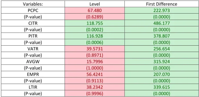
The descriptive statistics visualized in the previous section showed that there is significant variation in the variables of interest, especially across countries. There is, however, a positive time trend in our consumption variable. We therefore need to consider whether the variables represent stationary series or not. Regressing nonstationary series which are not cointegrated on each other can lead to spurious regressions which can be misleading. Spurious regressions seem highly significant and seem to have high goodness of fit but are in fact nonsensical. We test the stationarity of our variables using Individual Root – Fisher – Augmented Dickey Fuller (ADF) tests. The results are summarized in Table 3 below. Green means stationary and red means nonstationary.

Table 3: Results of Individual Root – Fisher – ADF tests

Variables: Level First Difference

PCPC 67.480 222.973 (P-value) (0.6289) (0.0000) CITR 118.755 486.177 (P-value) (0.0002) (0.0000) PITR 116.928 378.807 (P-value) (0.0006) (0.0000) VATR 39.5731 256.654 (P-value) (0.8971) (0.0000) AVGW 15.7996 315.924 (P-value) (1.0000) (0.0000) EMPR 56.4241 207.070 (P-value) (0.9113) (0.0000) LTIR 38.2342 339.615 (P-value) (0.9996) (0.0000)

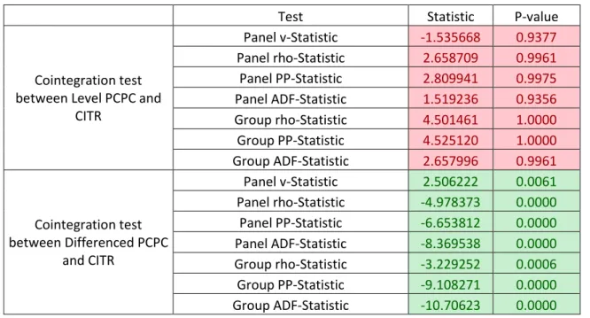
We see that most variables, and importantly the dependent variable PCPC, are not stationary in level terms but all variables are stationary in their first difference forms. Additionally, as can be seen in Table 4 our dependent variable PCPC and variable of interest CITR are not cointegrated in level terms while PCPC is not stationary and we therefore risk a spurious regression in level terms. However, as can also be seen in Table 4 where again all 7 different test statistics all indicate the same result, PCPC and CITR are cointegrated in their first difference forms. Variables being cointegrated means that there is a long-term or equilibrium relationship between the variables and thus that a regression of the variables is not spurious (Gujarati, 2009). Taken together, the results of the unit-root and cointegration tests indicate that we should use the first difference forms of the variables in our regressions and thereby that is what we do.

Table 4: Results of Panel Cointegration tests

Test Statistic P-value

Cointegration test between Level PCPC and

CITR Panel v-Statistic -1.535668 0.9377 Panel rho-Statistic 2.658709 0.9961 Panel PP-Statistic 2.809941 0.9975 Panel ADF-Statistic 1.519236 0.9356 Group rho-Statistic 4.501461 1.0000 Group PP-Statistic 4.525120 1.0000 Group ADF-Statistic 2.657996 0.9961 Cointegration test between Differenced PCPC and CITR Panel v-Statistic 2.506222 0.0061 Panel rho-Statistic -4.978373 0.0000 Panel PP-Statistic -6.653812 0.0000 Panel ADF-Statistic -8.369538 0.0000 Group rho-Statistic -3.229252 0.0006 Group PP-Statistic -9.108271 0.0000 Group ADF-Statistic -10.70623 0.0000

6. Econometric Model and Empirical Results

This section describes the econometric models used to test our hypotheses and the results of the models.

6.1 Econometric Models

In the previous section, we concluded that we would use differenced variables in our regression. We first consider a Pooled OLS Multiple Regression model on our panel data with all variables differenced. The equation for this model is as such:

Equation 3: Pooled OLS

∆𝑃𝐶𝑃𝐶𝑖𝑡 = 𝛽0+ 𝛽1∆𝐶𝐼𝑇𝑅𝑖𝑡+ 𝛽2∆𝑃𝐼𝑇𝑅𝑖𝑡+ 𝛽3∆𝑉𝐴𝑇𝑅𝑖𝑡+ 𝛽4∆𝐴𝑉𝐺𝑊𝑖𝑡 + 𝛽₅∆𝐸𝑀𝑃𝑅_𝑖𝑡+ 𝛽₆∆𝐿𝑇𝐼𝑅_𝑖𝑡+ 𝛽₇𝐷𝑈𝑀𝑀𝑌𝐹𝐶_𝑡+ 𝜀_𝑖𝑡

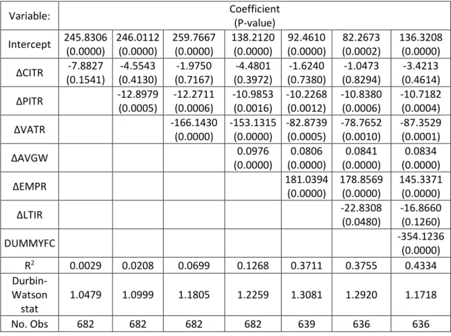
To show the effects of our control variables we add them sequentially and see their effects on CITR. The results of this process are summarized in Table 5 below and detailed output can be found in Appendix 5:

Table 5: Sequential Pooled OLS results

Variable: Coefficient (P-value) Intercept 245.8306 (0.0000) 246.0112 (0.0000) 259.7667 (0.0000) 138.2120 (0.0000) 92.4610 (0.0000) 82.2673 (0.0002) 136.3208 (0.0000) ΔCITR -7.8827 (0.1541) -4.5543 (0.4130) -1.9750 (0.7167) -4.4801 (0.3972) -1.6240 (0.7380) -1.0473 (0.8294) -3.4213 (0.4614) ΔPITR -12.8979 (0.0005) -12.2711 (0.0006) -10.9853 (0.0016) -10.2268 (0.0012) -10.8380 (0.0006) -10.7182 (0.0004) ΔVATR -166.1430 (0.0000) -153.1315 (0.0000) -82.8739 (0.0005) -78.7652 (0.0010) -87.3529 (0.0001) ΔAVGW 0.0976 (0.0000) 0.0806 (0.0000) 0.0841 (0.0000) 0.0834 (0.0000) ΔEMPR 181.0394 (0.0000) 178.8569 (0.0000) 145.3371 (0.0000) ΔLTIR -22.8308 (0.0480) -16.8660 (0.1260) DUMMYFC -354.1236 (0.0000) R2 _{0.0029 0.0208 0.0699 0.1268 0.3711 0.3755 0.4334} Durbin-Watson stat 1.0479 1.0999 1.1805 1.2259 1.3081 1.2920 1.1718 No. Obs 682 682 682 682 639 636 636

As can be seen in Table 5 there are no obvious causes for concern, in regard to that no variables are alternating signs nor are there any too large changes in the significance of the coefficients. All coefficients for the different variables have the expected sign in line with economic theory. The R-squared statistics are increasing with every variable added, meaning that the model’s fit to the data improves. The coefficient for our variable of interest ΔCITR is the main result of the regression models to be analyzed. It has the expected negative sign which a tax rate should have but is also insignificant in every model regressed. Some control variables like ΔAVGW and DUMMYFC increase the significance of ΔCITR and a regression with only those 3 explanatory variables yields a significant negative coefficient for ΔCITR as can be seen in Appendix 5. However, there is nothing to suggest that a model with only these 3 control variables would better explain consumption expenditure than a model with all of them. Thus, the result is still that the effect of ΔCITR on ΔPCPC is consistently insignificant. Importantly, all the other variables in the model are consistently significant with the exception of ΔLTIR in the model with all variables. The other two tax rates ΔPITR and ΔVATR are robustly significant.

When dealing with panel data one usually considers the use of a few different types of regression models. These are Pooled OLS, Random Effects Models (REM) and Fixed Effects Models (FEM). With Pooled OLS we estimate a regression model on all observations in the panel while disregarding that they come from different countries and that the same years are observed multiple times. Such a model has only one constant intercept. Random and Fixed Effects models are used to allow the different cross-sections or the different time points in a panel to have individual intercepts. This can be necessary in panel data regressions to estimate the true coefficients of different variables by controlling for unobserved heterogeneity. The difference between REM and FEM is that REM assumes the individual intercepts are random deviations from a common intercept for the larger population while FEM assumes that every cross-section or time period has its own intercept which is not a random deviation. On level data fixed effects can be used to control for unobserved heterogeneity, though we use differenced data and thereby that is already controlled for. Nevertheless, changes in different countries can still be affected by country-specific unobserved factors and for that reason REM and FEM can still be considered but are not necessarily required to obtain robust estimates. To decide if REM

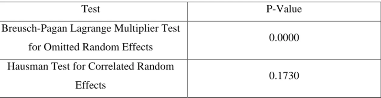
and FEM are suitable and to decide between them, the formal tests of the Lagrange Multiplier Test for Omitted Random Effects and the Hausman Test for Correlated Random Effects are used. The results of these tests are shown in Table 6 on the next page.

Table 6: REM and FEM testing

Test P-Value

Breusch-Pagan Lagrange Multiplier Test

for Omitted Random Effects 0.0000

Hausman Test for Correlated Random

Effects 0.1730

The Lagrange Multiplier Test for Random Effects conducted on the Pooled OLS model with all variables showed that a Random Effects Model is preferred over the Pooled OLS model. All different test statistics uniformly showed P-values of 0.0000. The test suggests using Random Effects both for cross-sections and for time periods. However, this is not possible with an unbalanced panel such as ours. Therefore, we choose to only use country Random Effects, partly because country effects are the most intuitive for this dataset and partly because we already control for one time effect in the form of the 2008-2009 financial crisis dummy variable. The functional form of our REM regression is:

Equation 4: REM Regression

∆𝑃𝐶𝑃𝐶𝑖𝑡 = 𝛽0𝑖+ 𝛽1∆𝐶𝐼𝑇𝑅𝑖𝑡+ 𝛽2∆𝑃𝐼𝑇𝑅𝑖𝑡+ 𝛽3∆𝑉𝐴𝑇𝑅𝑖𝑡+ 𝛽4∆𝐴𝑉𝐺𝑊𝑖𝑡+ 𝛽₅∆𝐸𝑀𝑃𝑅_𝑖𝑡 + 𝛽₆∆𝐿𝑇𝐼𝑅_𝑖𝑡+ 𝛽₇𝐷𝑈𝑀𝑀𝑌𝐹𝐶_𝑡+ 𝜀_𝑖𝑡 where 𝛽_𝑜𝑖 = 𝛽_𝑜+ 𝜀_𝑖

The Intercept now has a subscript i, meaning that each cross-section, each country, will have an individual intercept which is assumed to be a random deviation from the common intercept. A Hausman Test for Correlated Random Effects is conducted on the REM to see if FEM is preferred. The result as can also be seen in Table 6 is that FEM is not preferred over REM and REM is the model we will base our main analysis on. Though as can be seen in Appendix 6, the coefficient for our variable of interest ΔCITR significantly differs between REM and FEM and we will therefore show the results of the FEM also to verify that the main result still does not differ even with that model.

6.2 Empirical Results

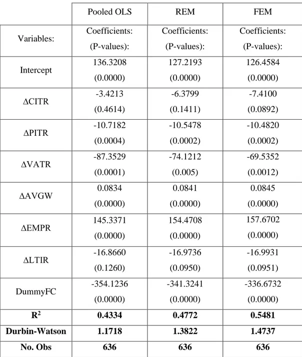
Table 7 on the next page shows the comparison between Pooled OLS, REM and FEM regression models on our data with all control variables included. The Random Effects

Model is according to earlier testing the best model. Regardless, the three models show the same main result and thus reinforce each other.

Table 7: Regression results

Pooled OLS REM FEM

Variables: Coefficients: (P-values): Coefficients: (P-values): Coefficients: (P-values): Intercept 136.3208 (0.0000) 127.2193 (0.0000) 126.4584 (0.0000) ∆CITR -3.4213 (0.4614) -6.3799 (0.1411) -7.4100 (0.0892) ∆PITR -10.7182 (0.0004) -10.5478 (0.0002) -10.4820 (0.0002) ∆VATR -87.3529 (0.0001) -74.1212 (0.005) -69.5352 (0.0012) ∆AVGW 0.0834 (0.0000) 0.0841 (0.0000) 0.0845 (0.0000) ∆EMPR 145.3371 (0.0000) 154.4708 (0.0000) 157.6702 (0.0000) ∆LTIR -16.8660 (0.1260) -16.9736 (0.0950) -16.9931 (0.0951) DummyFC -354.1236 (0.0000) -341.3241 (0.0000) -336.6732 (0.0000) R2 _{0.4334 0.4772 0.5481} Durbin-Watson 1.1718 1.3822 1.4737 No. Obs 636 636 636

The table shows our main findings and will be the basis for our analysis in the next chapter. Briefly described, the coefficient for ΔCITR is consistently, including in the REM, insignificant. Meanwhile, the other variables except ΔLTIR are all highly significant on all conventional significance levels in economics and their coefficients are robust across the three models.

6.3 Robustness Tests

Several tests were made previously do determine which method would be suitable for our data. Concerns about stationarity and cointegration, as well as effects testing, has been addressed.

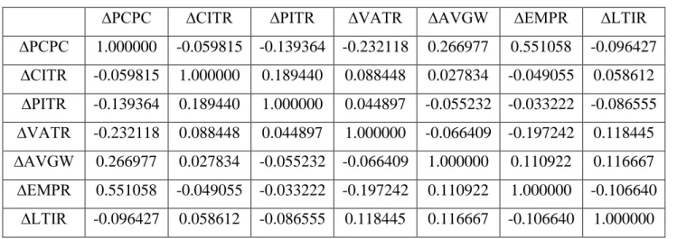
Multicollinearity can be a problem in multiple regression analysis. Multicollinearity occurs when some explanatory variables in the model are highly linearly correlated with one another. This can cause uncertainty in estimating the individual coefficient estimates of the correlated variables. Multicollinearity can be detected through checking if the correlation between any two explanatory variables is too high in a correlation matrix and through checking if the Variance Inflation Factors (VIF) are too high. Table 8 and Table 9 below shows the correlation matrix and VIF’s respectively for the REM.

Table 8: Correlation Matrix

∆PCPC ∆CITR ∆PITR ∆VATR ∆AVGW ∆EMPR ∆LTIR

∆PCPC 1.000000 -0.059815 -0.139364 -0.232118 0.266977 0.551058 -0.096427 ∆CITR -0.059815 1.000000 0.189440 0.088448 0.027834 -0.049055 0.058612 ∆PITR -0.139364 0.189440 1.000000 0.044897 -0.055232 -0.033222 -0.086555 ∆VATR -0.232118 0.088448 0.044897 1.000000 -0.066409 -0.197242 0.118445 ∆AVGW 0.266977 0.027834 -0.055232 -0.066409 1.000000 0.110922 0.116667 ∆EMPR 0.551058 -0.049055 -0.033222 -0.197242 0.110922 1.000000 -0.106640 ∆LTIR -0.096427 0.058612 -0.086555 0.118445 0.116667 -0.106640 1.000000

Table 9: Variance Inflation Factors

Variables: Uncentered VIF Centered VIF

Intercept 1.539057 NA ∆CITR 1.056082 1.054305 ∆PITR 1.051389 1.051377 ∆VATR 1.072801 1.067911 ∆AVGW 1.467776 1.044447 ∆EMPR 1.256058 1.228847 ∆LTIR 1.072462 1.060041 DummyFC 1.203130 1.164082

As a rule of thumb, no correlation coefficient should be above 0.9 and no VIF should be above 10. Both these conditions are met and thereby we conclude that there is no multicollinearity problem.

Autocorrelation in the regression residuals is a potential problem in regression models which violate regression assumptions and can cause inefficient estimates. For example, our conclusion that ΔCITR has an insignificant effect in the model can be incorrect if autocorrelation causes the standard errors to be inefficient. We can check for the presence of autocorrelation in the first lag with the Durbin-Watson d-statistic. A d-statistic close to 2 implies no autocorrelation in the first lag and significantly lower statistics imply positive first order autocorrelation and significantly higher statistics imply negative first order autocorrelation. The lower critical value for a regression such as ours with 8 regressors (including intercept) and 636 observations is approximately 1.846. As can be seen in Table 7 the d-statistic is 1.3822 for the REM and the other models also exhibit values below the critical value. Therefore, we cannot rule out that there is positive autocorrelation in our models. We can remedy this problem by using the FEM and adding an autoregressive term in the form of the lagged dependent variable ∆PCPCt-1 as an explanatory variable.

Table 10: Autocorrelation Corrected FEM Regression Output

Variable: Coefficient (P-value)

Intercept 144.6017 (0.0000) ∆CITR -6.5117 (0.1109) ∆PITR -5.3217 (0.0322) ∆VATR -42.3685 (0.0292) ∆AVGW 0.0695 (0.0000) ∆EMPR 143.2696 (0.0000) ∆LTIR -23.0582 (0.0147) DummyFC -414.3052 (0.0000) ΔPCPCt-1 0.3418 (0.0000) R-squared 0.6038

Durbin-Watson 2.0670

No. Obs 600

In Table 10 and more detailed in Appendix 7, the output for this regression can be seen. Its VIF’s are also shown in Appendix 7 to confirm that the model does not become multicollinear. That regression exhibits a d-statistic of about 2.0670. Because (4 - 2.0670) is higher than the lower critical value of 1.846 we no longer find evidence of first order autocorrelation in the residuals. The coefficients in the modified model change in magnitude somewhat but not in sign nor significance. The result is still that ΔCITR has a statistically insignificant effect on ΔPCPC while the other variables generally do.

Heteroscedasticity is also a potential problem in regression models which violate regression assumptions and can cause inefficient estimates, much like autocorrelation. Heteroscedasticity occurs when the variance of the residuals is dependent on some explanatory variable. We are not able to formally test for heteroscedasticity in our unbalanced panel regressions. Therefore, we conduct an informal test in the form of a graphical examination. We plot the residuals of the REM against the fitted values of the REM and check if the variance looks constant across the fitted values. Generally, the residuals can be contained within a rectangular shape meaning that the variance seems constant. There are some outliers, but only a couple that do not fit. Thus, we do not find evidence to suggest that we have a heteroscedasticity problem.

Figure 5: Graphical test for Heteroscedasticity

-2500 -2000 -1500 -1000 -500 0 500 1000 1500 -2000 -1500 -1000 -500 0 500 1000 1500

RESIDUALPLOT

7. Analysis and Discussion of the Results

In this chapter, the empirical results presented in the previous chapter will be analyzed and used to evaluate our hypotheses. The implications of the results through the lens of the theoretical framework will also be discussed, as well as the robustness of the results.

The first hypothesis was that “the tax rate on dividend capital income will not have a significant effect on aggregate consumption expenditure”. Analyzing the sequential OLS process depicted in Table 5, the results regarding the effect of the dividend capital income tax rate on private consumption expenditure do point in a unilateral direction. We see that the coefficient for ΔCITR is consistently insignificant in every model, regardless of which control variables were added. Because the effects of the different control variables on the magnitude and significance of ΔCITR varies, different orders of the addition of the control variables could produce models where ΔCITR’s coefficient is significant. However, as previously mentioned there is nothing to indicate that a model with only some of the control variables is better. ΔLTIR is also insignificant in the model with all variables included but it does not significantly change the coefficient for ΔCITR regardless. The coefficients for the control variables chosen have proven to be robust throughout the different model specifications, this can be seen in Table 5 when the variables are sequentially added to the regression. The coefficients for ΔAVGW and ΔPITR do not change much when more variables are included. This we would say is a desirable attribute of control variables. Further, almost all the control variables’ coefficients are significant, only LTIR´s coefficient is insignificant. As Table 7 shows, the model specification suggested by testing, REM, and the alternative effects specifications of Pooled OLS and FEM all yield similar results. The coefficient for ΔCITR is consistently insignificant. As such, the REM we consider to be correctly specified, other specifications we could consider, as well as the autocorrelation corrected model all yield insignificant coefficient estimates for ΔCITR. Therefore, based on our empirical models we do not reject the first hypothesis that the tax rate on dividend capital income does not have a significant effect on aggregate consumption expenditure.

The second hypothesis was that “the tax rates on dividend capital income, labor income and consumption should have a negative effect on aggregate consumption expenditure, though not all necessarily significant”. According to neoclassical economic theory, taxes

decrease disposable income and thereby reduces the base for consumption expenditure. Analyzing primarily the chosen REM and autocorrelation corrected model all the coefficients for the tax rates are negative. The coefficient for ΔCITR is insignificant as previously discussed. The coefficients for ΔPITR and ΔVATR are both highly significant and their estimates are robust in the sequential OLS process and across the different effects specifications. This taken together, based on our empirical models we do not reject the second hypothesis.

The third hypothesis was that “the tax rate on dividend capital income has a weaker effect on aggregate consumption expenditure than the tax rate on labor income and the VAT rate”. This hypothesis has been relatively uncontradicted according to the results from our chosen models, both in the aspect of magnitude and significance, ΔPITR´s and ΔVATR´s coefficient estimates are larger in magnitude than for ΔCITR´s. Furthermore, since the coefficient for ΔCITR is insignificant its effect is deemed to be zero while the coefficients for ΔPITR and ΔVATR are highly significant. As such, the effect of CITR on private consumption expenditure must be considered weaker than that of the other two tax rates. Therefore, based on our empirical models we do not reject the third hypothesis.

While we have analyzed the implications of the empirical results for the hypotheses, the results can also be analyzed through the lens of the theory and previous empirical work. In the theoretical section we reviewed different possible economic mechanisms to explain how the tax rate on capital income could affect consumption expenditure and how it may not. However, it is important to note that the method employed in this thesis is not sufficient to identify which specific mechanisms are in effect. Nevertheless, the group of mechanisms that could explain are important to all cover in the theoretical framework, even if one or a few cannot be identified as the specific cause. We can however discuss the likelihood that some theory seems to better describe the empirical results. One central feature of our empirical results is the lower magnitude and insignificant coefficient estimate for the tax rate on dividend capital income compared to the highly significant coefficient estimate for the tax rate on labor income. The possible implications of this for the different theoretical mechanisms presented in chapter 2 will be discussed.

A typical Keynesian consumption function as presented in 2.1.2 could partly explain our empirical results. The significant negative coefficient of the tax rate on labor income is in

line with the theory while the coefficient for our variable of interest, the tax rate on dividend capital income, is not. This could be because of the potentially lower marginal propensity to consume for the commonly wealthier recipients of capital income or simply because labor income is so much of a larger share of the majority of people’s income (OECD, 2015). Souleles (1999) found excess sensitivity of consumption to tax changes which was believed to be due to a higher marginal propensity to consume among liquidity constrained low-income households. This could be said to fall in line with, or at least not contradict, our results since dividend income recipients are on average less liquidity constrained and may therefore not react as much to tax changes.

Previous empirical studies such as Haug (2020) and Hayo & Neumeier (2017) generally did not find support for Ricardian Equivalence and studies like Poterba (1988) and Souleles (2002) generally did not find support for the Permanent Income Hypothesis. Our results could also be considered in line with these findings, since we find significant effects on consumption of the tax rate on labor income. It is the tax rate on dividend income which is not in line with the previously observed sensitivity of consumption to tax rate changes. Though we do not deem it likely that this is because theories like Ricardian Equivalence and the Permanent Income Hypothesis describe our results. These theories do not explain why the conclusion should be different regarding labor and capital income and therefore do not seem as applicable.

Generally, since the conclusions about the effects of the two tax rates are opposite, we could suspect that some factor which is specific to capital income and its taxation is in effect. The possibilities of tax planning discussed in the theory section is one such factor. We cannot say which specific theoretical mechanism is in effect to explain the reason for our results. However, since we have differing results for capital and labor income tax rates, some form of tax planning which is more common regarding capital income, seems to be a more likely explanation for our results. One potential tax planning related mechanism which could be in effect is that of income shifting. Since consumption is not affected, it seems money is perhaps not moved to other countries as a result of tax rate changes but perhaps rather that the label of the income within the country is changed and thus withdrawn anyway. This could mean that one would see significant changes in the amount of dividends paid out in response to dividend tax rate changes.

8. Conclusions

We have investigated if the overall corporate income tax rate plus private dividend tax rate significantly affects aggregate consumption expenditure in the OECD countries during the period 2000-2019. Our results indicate that the overall tax rate on dividend capital income does not affect aggregate private consumption expenditure in the OECD countries during the period 2000-2019. Several model specifications estimated using differenced data, which we deemed to be the correct form, all produced insignificant coefficients for the dividend capital income tax rate’s effect on consumption expenditure. The tax rate on labor income as well as the VAT rate on the other hand were found to have significant effects on consumption expenditure. Thus, we did not reject any of our three hypotheses.

The possible implications of these results are that the tax rate on dividend capital income could be changed with the largest effect occurring to the individuals owning the assets and not the economy as a whole because of consumption effects. This insight could be considered by policymakers who evaluate the efficiency of tax policies or who pursue new efficient tax policies, and thus may want to change tax rates on dividend income.

This leaves room for much further research into the topic of capital income taxation and its effects on private consumption expenditure. Other types of capital income derived from different types of assets could be studied. The other side of earnings derived from the ownership of shares of companies are capital gains. The taxation of capital gains is an important part of capital taxation and would perhaps show a different side of this subject. It could to a greater extent illuminate the role of tax planning schemes, such as refraining from realization of capital gains. Additionally, studying a specific capital income tax reform could also help identify consumption effects.