Insights into Criteria for Statistical Significance from Signal Detection Analysis

(1)

Meta-Psychology, 2019, vol 3, MP.2018.871, https://doi.org/10.15626/MP.2018.871 Article type: Original Article Published under the CC-BY4.0 license

Open data: Not applicable Open materials: Yes

Open and reproducible analysis: Yes Open reviews and editorial process: Yes Preregistration: No

Edited by: Daniël Lakens

Reviewed by:Patrick R Heck, Angelika Stefan, Felix Schönbrodt

Analysis reproduced by: Jack Davis

All supplementary files can be accessed at OSF: https://doi.org/10.17605/OSF.IO/69XMG

Insights into Criteria for Statistical Significance from Signal

Detection Analysis

Jessica K. Witt

Colorado State University

What is best criterion for determining statistical significance? In psychology, the criterion has been p < .05. This criterion has been criticized since its inception, and the criticisms have been rejuvenated with recent failures to replicate studies published in top psychology journals. Several replacement criteria have been suggested including reducing the alpha level to .005 or switching to other types of criteria such as Bayes factors or effect sizes. Here, various decision criteria for statistical significance were evaluated using signal detection analysis on the outcomes of simulated data. The signal detection measure of area under the curve (AUC) is a measure of discriminability with a value of 1 indicating perfect discriminability and 0.5 indicating chance performance. Applied to criteria for statistical significance, it provides an estimate of the decision criterion’s performance in discriminating real effects from null effects. AUCs were high (M = .96, median = .97) for p values, suggesting merit in using p values to discriminate significant effects. AUCs can be used to assess methodological questions such as how much improvement will be gained with increased sample size, how much discriminability will be lost with questionable research practices, and whether it is better to run a single high-powered study or a study plus a replication at lower powers. AUCs were also used to compare performance across p values, Bayes factors, and effect size (Cohen’s d). AUCs were equivalent for p values and Bayes factors and were slightly higher for effect size. Signal detection analysis provides separate measures of discriminability and bias. With respect to bias, the specific thresholds that produced maximally-optimal utility depended on sample size, although this dependency was particularly notable for p values and less so for Bayes factors. The application of signal detection theory to the issue of statistical significance highlights the need to focus on both false alarms and misses, rather than false alarms alone.

Keywords: Statistical significance, Bayes factor, Effect size, p values

Jessica K. Witt, Department of Psychology, Colorado State University, Fort Collins, CO 80523.

The author would like to thank Anne Cleary, John Wixted, Mark Prince, Susan Wagner Cook, Mike Dodd, Art Glenberg, Jim Nairne, Jeremy Wolfe, and Ben Prytherch for useful discussions and feedback on an earlier draft. The author would also like to thank the editor (Daniel Lakens) and reviewers (Patrick Heck, Angelika Stefan, Felix Schönbrodt, and Daniel Benjamin) for valuable suggestions. This work was supported by grants from the National Science Foundation to JKW (BCS-1348916 and BCS-1632222).

Please address correspondence to Jessica Witt, Colorado State University, Behavioral Sciences Building, Fort Collins, CO 80523 USA. Email: Jessica.Witt@colostate.edu.

(2)

WITT

2

Scientists across many disciplines including psychology, biology, and economics use p < .05 as the criterion for statistical significance. This threshold has recently been challenged due to numerous failures to replicate findings published in top journals (Begley & Ellis, 2012; Camerer et al., 2016; Open Science Collaboration, 2015). Changes in the recommendations for statistical significance include using a stricter criterion for significance (e.g., p < .005; Benjamin et al., 2017) and minimizing flexibility in decisions around data collection and analysis (e.g., Simmons, Nelson, & Simonsohn, 2011). These recommendations were designed to increase replicability by decreasing the false alarm rates, which is the rate at which null effects are incorrectly labeled as significant. However, the best criteria for statistical significance are ones that maximize discriminability between real and null effects, not just those that minimize false alarms. One analytic technique that is intended to measure the discriminability of a test is signal detection theory (Green & Swets, 1966). Signal detection theory has previously been applied to evaluate p values (Krueger & Heck, 2017). Here, the signal detection theory measure of area under the curve (AUC) is offered as a tool to quantify the effectiveness of various measures of statistical effects.

Signal detection analysis involves categorizing outcomes into four categories. Applied to criteria for statistical significance, a hit occurs when there is a true effect and the analysis correctly identifies it as significant (see Table 1). A miss occurs when there is a true effect but the analysis identifies it as not significant. A correct rejection occurs when there is no effect and the analysis correctly identifies it as not significant, and a false alarm occurs when there is no effect but the analysis identifies it as significant. In statistics, Type I errors (false alarms) and Type II errors (misses) are sometimes considered separately, with Type I errors being a function of the alpha level and Type II errors being a function of power. An advantage of signal detection theory is that it combines Type I and Type II errors into a single analysis of discriminability and also

1_{This number was selected somewhat arbitrarily, and}

the results generalized to other numbers. Larger number of repeats reduced the standard deviations of the results reported below, but did not affect the means. The decision to simulate sets of studies was to allow for

considers the relative distributions of each type of error in the analysis of bias.

Data Simulations for Experiment 1

Data were simulated for two independent groups of 64 participants each, which corresponds to 80% power at an alpha level of .05 for a two-tailed independent-samples t-test.

Table 1. Signal detection classification of data based on

the example criteria p < .05 for a true effect (Cohen’s d = 0.50) and a null effect (Cohen’s d = 0).

P < .05 P > .05 “Significant” “Not Significant”

d =.50 Hit Miss

d = 0 False Alarm _RejectionCorrect

Data for one group was sampled from a normal distribution with a mean of 50 and a standard deviation of 10 (such as might be found on a memory test with a total score of 100). The data for the other group was sampled from a normal distribution with a mean of 50 (for studies with a null effect) or 45 (for studies with an effect size of Cohen’s d = .50) and a standard deviation of 10. The data were submitted to an independent-samples t-test (all simulations and analyses were conducted in R; R Core Team, 2017). Details of the simulation are available in the

online supplementary materials

(https://osf.io/bwqm8/). This initial simulation will be referred to as Experiment 1. See appendix for overview of all of experiments.

Data were simulated from 20 studies1_{, half of} which had an effect size of 0 and half had a medium effect size (Cohen’s d = .50). The result from each simulated study was classified as a hit or miss (for studies modeled as a medium effect) or as a correct rejection or false alarm (for studies modeled as a null effect). The classification was based on four criteria for statistical significant related to p values: p < .10, p < .05, p < .005, and p < .001. This process was

multiple comparisons across a variety of measures (p values, Bayes factors, and effect sizes).

(3)

INSIGHTS INTO CRITERIA FOR STATISTICAL SIGNIFICANCE FROM SIGNAL DETECTION ANALYSIS 3

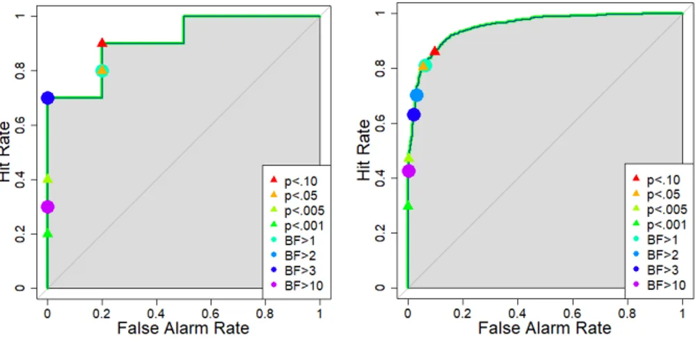
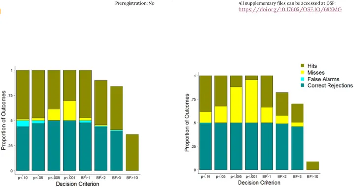
repeated 100 times1_{. The outcomes across all} studies were summarized into the proportions of hits, misses, false alarms, and correct rejections for each criterion (see Figure 1). In addition, the hit rates and false alarm rates were calculated for the purpose of plotting the receiver operator characteristic (ROC) curves (see Figure 2). The hit rate is the proportion of studies for which the simulated effect was real and the criterion classified it as significant, and the false alarm rate is the

proportion of studies for which the simulated effect was null but the criterion classified it as significant. To clarify, whereas the proportion of hits (as plotted in Figure 1) is the number of hits divided by the total number of studies, the hit rate (plotted in Figure 2) is the number of hits divided by the number of studies modeled as a real effect. Bayes factors, which are also plotted, are discussed below.

Figure 1. Proportion of each outcome as a function of the decision criterion for significance. Brighter colors correspond

to errors and dark colors correspond to correct classifications. For criteria of Bayes factors greater than 2, 3, or 10, studies that produced a Bayes factor less than the criterion but greater than the inverse of the criterion were considered inconclusive, which is why the total proportion of outcomes does not equal 1.

Figure 2. Mean hit rates are plotted as a function of mean false alarm rates and the decision criterion (see legend) for

one set of 20 studies (left panel) and averaged across all 100 sets of 20 studies (right panel). ROC curves are plotted for criteria based on p values (thick green line) and Bayes factor (thin blue line). The two lines are identical (as was the case for all 100 sets of 20 studies). Area under the curve (AUC) is the shaded area.

(4)

In selecting a criterion for statistical significance, researchers must select a measure (e.g., p values) and a threshold within that measure (e.g., alpha = .05). A measure can be evaluated by assessing its ability to discriminate between real and null effects, which can be quantified by calculating the area under the ROC curve (AUC; Macmillan & Creelman, 2008). With respect to evaluating thresholds for a specific measure (e.g., comparing .005 to .05), the location of each threshold on the ROC curve can be calculated. Location on the curve is a measure of bias. Each of these measures will be considered in turn.

To measure discriminability of p values, the AUC was computed 100 times, once for each set of 20 studies. Unlike the discriminability measure of d’, the discriminability measure of AUC makes no assumptions regarding the underlying distributions, which is critical because distributions of p values are not normally distributed. Higher AUCs indicate better ability to discriminate real effects from null effects. If discrimination were perfect, the curve would follow the left and top boundaries in Figure 2, and the AUC would equal 1 (i.e. the entire area would be under the curve). If discrimination were at chance, the curve would follow the diagonal line in Figure 2, and the AUC would be .5 (i.e. only 50% of the area would be under the curve). As is apparent in Figure 2, p values produced curves that were closer to 1 (perfect performance) than to .5 (chance performance). The mean AUC was .96 (median = .97, SD = .04). Thus, p values were effective, though not perfect, at discriminating between real and null effects. This aligns with conclusions from other valuations of p values (e.g., Krueger & Heck, 2017, 2018). These AUC values suggest some benefit in using p values, at least as a continuous measure without necessarily having strict thresholds for significance (McShane, Gal, Gelman, Robert, & Tackett, 2018). Perhaps alternative methods to reduce false alarm rates might be more beneficial than to eliminate p values altogether (e.g., Trafimow & Marks, 2015). Note that measures of discriminability evaluate p values as a measure without consideration of the specific alpha value

adopted as the criterion. Specific alpha levels relate to bias, and are discussed below.

What could improve discriminability when using

p values as the criterion for statistical significance?

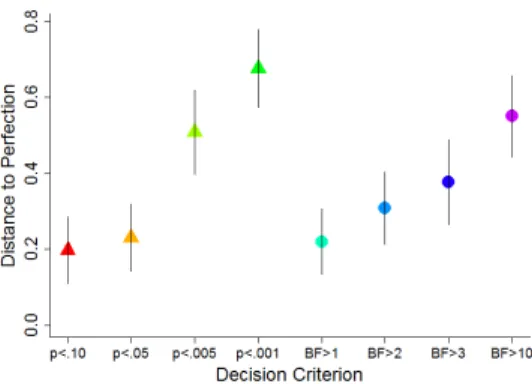
One suggestion has been to lower the threshold from .05 to .005. This would not alter the discriminability because discriminability relates to p values as a whole, not to specific thresholds. Thresholds refer to locations on the curve, and these dictate bias, rather than discriminability. Signal detection theory distinguishes between discriminability and bias. As applied to the case of criteria for statistical significance, discriminability refers to the criterion’s performance at identifying real effects versus null effects, and bias refers to whether the errors tend to be false alarms or misses. Assessing bias can be useful for selecting the appropriate criterion for asserting statistical significance. For example, assume that the cost of a miss is equivalent to the cost of a false alarm in a particular field. In that case, optimal utility would be achieved by setting the criterion in such a way that its point on the ROC curve is the one that falls closest to the upper left corner in Figure 2. The Euclidean distance between each point on the ROC curve and the point of perfect performance is plotted in Figure 3. For the scenario that was simulated, an alpha level closer to the blue dot, which aligns with an alpha level of .10, would come closer to achieving that maximum-utility outcome than an alpha level of .005. Lowering the criterion for statistical significance to p < .005 would increase the number of studies that will replicate by decreasing false alarms, but it would do so at the cost of missing real effects (see also Krueger & Heck, 2017). Note the proportion of misses in Figure 1 across the various criteria, particularly for the criterion of p < .005. Misses are bad for science (Fiedler, Kutzner, & Krueger, 2012; Murayama, Pekrun, & Fiedler, 2014). Assuming that null effects are theoretically interesting and practically important, it is important to determine which null effects are due to a genuine lack of difference versus a miss of a true effect. Is the trade-off to increase replicability worth the large increase in misses?

(5)

Perhaps science can adopt alternative means to improve replicability without sacrificing so many missed hits, such as increasing incentives for publishing statistically- and scientifically-sound significant findings and also publishing (statistically- and scientifically-sound) null results.

Figure 3. Distance to perfection was calculated as the

Euclidean distance between each point on the ROC curve (see Figure 2) and the top-left corner (which corresponds to 100% hit rate and 0% false alarm rate) across all 100 sets of 20 studies. A lower distance to perfection score indicates better discriminability between real and null effects. Error bars represent 95% confidence intervals.

One effective way to improve replicability is to increase sample size. Many studies are underpowered (e.g., Etz & Vandekerckhove, 2016; Fraley & Vazire, 2014; Ioannidis, 2005; Sedlmeier & Gigerenzer, 1989). The simulations in Experiment 1 showed that at a power of 80% (at an alpha level of .05), the mean AUC for p values was .96. At a power of 50%, the mean AUC for p values was .85 (median = .87; SD = .10). Increasing power to 90% produced a mean AUC of .975 (median = .99; SD = .03), increasing power to 95% produced a mean AUC of .984 (median = 1; SD = .03), and increasing power to

99% produced a mean AUC of .999 (median = 1; SD = .004). If resources are unlimited, increasing sample size to increase power is an effective way of improving discriminability of real effects from null effects (Krueger & Heck, 2017).

Assuming limited resources, one might wonder whether it is better to run one high-powered study or a study plus a replication that are both at 80% power. AUCs can help a researcher make these decisions. Two additional “experiments” (i.e., sets of simulations) were conducted. In Experiment 2, everything was the same as in Experiment 1 except the sample size for each group was 105 (which corresponds to 95% power at an alpha level of .05). In Experiment 3, everything was the same as in Experiment 1 except that for every study that was simulated, a second study with the same parameters was simulated and the higher p value was retained. This emulates a situation for which a study is conducted that produces a significant p value and then a replication fails to find a significant effect, so the effect is considered not significant. This is why the higher p value was retained. The mean AUC for Experiment 2 was .99 (median = 1; SD = .01). The mean AUC for Experiment 3 was .97 (median = .99;

SD = .04). This suggests that higher power produces

better discriminability than replicating a study with both the original and replication studies at 80% power. However, the higher-powered study produced more false alarms whereas the study plus replication produced few false alarms but more misses (see Figure 4). Again, researchers will need to decide what trade-offs between false alarms and misses make the most sense for their science.

(6)

Figure 4. Proportion of each outcome as a function of the decision criterion and whether one or two studies were run.

The left panel shows the outcomes across 100 sets of 20 studies, each with 105 data points per group (which

corresponds to 95% power at alpha = .05). The right panel shows the outcomes across 100 sets of 20 studies. For each study, a replication was conducted. Both the original study and the replication had 64 data points per group (which corresponds to 80% power at alpha = .05). In order for an effect to meet the decision criterion, both the original study and the replication had to produce values that exceeded the decision criterion. For example, for the criterion of p < .05, both the study and the replication had to produce p values < .05, otherwise the set of studies was considered not significant.

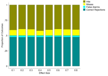
Power, rather than effect size, is more important for discriminability. In Experiment 4, data were simulated at 80% power (at an alpha of .05) for each of 8 effect sizes ranging from d = .1 - .8. The AUCs for each were approximately the same (M = .95; range of means for each effect size = .947 - .961; variations due to chance rather than systematic differences). As shown in Figure 5, when power was consistent, there were also no substantial differences in the rate of the different outcomes. Thus, while studying bigger effects will reduce the number of participants needed, it will not improve discriminability on its own.

Questionable Research Practices

Some recommendations to improve replicability concern practices to avoid. These have been labeled questionable research practices, and have been identified as particularly problematic (Simmons et al., 2011). AUCs can be used to assess the degree to which doing various questionable research practices reduces discriminability. One recommendation is to designate the number of participants to be run ahead of time, rather than use an optional stopping rule (Simmons et al., 2011).

In a new set of simulations (Experiment 5), each simulated study was conducted with 30 participants per group with either a Cohen’s d = .50 or d = 0. A lower sample size was used given that published studies tend to be underpowered

(7)

Figure 5. Proportion of SDT outcomes is plotted as a

function of effect size for the single criterion for

statistical significance of p < .05. Data were all simulated at a power of 80% at an alpha of .05.

As in Experiment 1, 20 studies were simulated, and this was repeated this 100 times. To try to mimic typical use of the optional stopping rule, for each study, if the p value was between .20 and .05, an additional 10 participants were added per group. After this addition, if the p value was less than .05, data collection stopped; otherwise the process was repeated up to 9 more times. On average, p-hacking in the form of adding more participants occurred 4.3 times in each set of 20 studies (SD = 2; Range = 0 – 11). The optional stopping rule produced differences in the AUCs relative to the original sample, but the differences were not systematic. Sometimes running additional unplanned participants improved discriminability and other times it worsened discriminability (see Figure 6). How can this questionable research practice have no impact the discriminability of real effects from null effects? The reason is that these questionable research practices increase the false alarm rate but they also increase the hit rate (see Figure 7). Much of the attention on the replication crisis has sought to minimize false alarms, but it is also necessary to discuss the corresponding increase in the number of misses (i.e. the decrease in the number of hits). Discriminability between real effects and null effects takes into account both the false alarm rate and the hit rate.

Figure 6. The area under the curve (AUC) for hacked

studies plotted as a function of the AUC for the original studies. A higher AUC indicates better discrimination between real and null effects. The line is at unity. Data points above the line indicate better discriminability for the hacked studies, and data points below the line indicate better discriminability for the original studies.

A decreased hit rate directly corresponds to an increased miss rate. Furthermore, the data were simulated so that the studies were underpowered. Although p-hacking increased the false alarm rates (see also Ioannidis, 2005), adding participants increased power, which is good for discriminability. To be clear, the recommendation is not to p-hack by running participants until the effect is significant. Instead, experiments should be run with sufficient power or only allow restricted flexibility in stopping data collection such as, for example, by following the recommendations of Lakens (2014) or using sequential Bayes Factor with a minimum and maximum N (Schönbrodt & Wagenmakers, 2018). But with respect to interpreting published research, the current simulations suggest that flexibility in data collection via an optional stopping rule does not necessarily void the findings (see also Murayama et al., 2014; Salomon, 2015). In these simulations, p-hacking increased the hit rate by 28% while only increasing the false alarm rate by 12%. Note, however, that p-hacking via optional stopping rules does not always increase hit rates more than false alarm rates. If power is high (e.g., > 99%), simulations showed that hit rates increased from

(8)

WITT

8

99.9% to 100% but false alarm rates increased from 5.4% to 9.8%.

Figure 7. Proportion of hits, false alarms, misses, and

correct rejections as a function of whether the studies were the original sample of 30 data points per group or had been p-hacked via an optional stopping rule. Outcomes shown only for the decision criterion of p < .05. Note that the seeming benefit for p-hacking is dependent on the low power of the simulated study.

Bayes Factor Versus p values

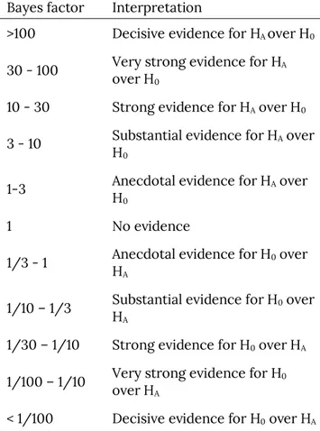
An alternative to p values is to use Bayes factors (e.g., Dienes, 2011; Kass & Raftery, 1995; Kruschke, 2013; Lee & Wagenmakers, 2005; Rouder, Speckman, Sun, Morey, & Iverson, 2009). Bayes factor refers to the ratio of likelihoods of the data for the alternative hypothesis relative to the null hypothesis. A Bayes factor of 1 corresponds to equal likelihood for the alternative and the null hypotheses, and a Bayes factor greater than 1 is evidence for the alternative hypothesis relative to the null hypothesis. Bayes factors quantify how well a hypothesis predicts the data relative to a competing hypothesis (such as the null hypothesis), and thus is a continuous measure for which the focus is on the strength of the evidence, rather than a specific cut-off for deeming effects significant or not. However, Bayes factors between 1-3 are considered weak or anecdotal evidence, so a Bayes factor of 3 could be considered a decision criterion akin to a criterion for significance (see Table 2), though not everyone

agrees with the idea of using strict cut-offs (e.g., Morey, 2015).

Table 2. Overview of relationship between Bayes factor

and conclusion about the evidence being in favor of the alternative hypothesis (HA) or the null hypothesis (H0).

Adapted from Wetzels et al. (2011), Lakens (2016), and Jeffreys (1961).

Bayes factor Interpretation

>100 Decisive evidence for HA over H0 30 - 100 Very strong evidence for HA

over H0

10 - 30 Strong evidence for HA over H0 3 - 10 Substantial evidence for HA over

H0

1-3 Anecdotal evidence for HA over H0

1 No evidence

1/3 - 1 Anecdotal evidence for H0 over HA

1/10 – 1/3 Substantial evidence for H0 over HA

1/30 – 1/10 Strong evidence for H0 over HA 1/100 – 1/10 Very strong evidence for H0

over HA

< 1/100 Decisive evidence for H0 over HA

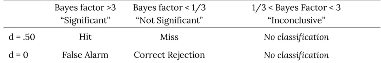
To measure discriminability and bias for Bayes factors, the studies simulated in Experiment 1 were also evaluated using four decision criteria related to Bayes factor (BF): BF > 1, BF > 2, BF > 3, and BF > 10. Studies were classified as shown in Table 3. Note that for Bayes factors that fell in between the criterion and its inverse (e.g., 1/3 – 3), no classification was made because the data were inconclusive. This is why the outcomes do not sum to 1 in Figure 1. The calculation of the AUCs is a function of the Bayes factor itself, rather

(9)

Table 3. Signal detection classification of data based on the example criteria Bayes factor > 3 for a true effect (Cohen’s d

= 0.50) and a null effect (Cohen’s d = 0).

Bayes factor >3 “Significant” Bayes factor < 1/3 “Not Significant” 1/3 < Bayes Factor < 3 “Inconclusive”

d = .50 Hit Miss No classification

d = 0 False Alarm Correct Rejection No classification

than classifications of outcomes, so even though not all studies could be classified into the four SDT outcomes, all studies contributed to the AUC calculation. The BayesFactor R package (Morey, Rouder, & Jamil, 2014) was used to calculate the Bayes factors. The default Cauchy prior was used when calculating Bayes factors, but different priors produced the same AUC results. Changing the prior produced shifts along the ROC curve but did not change discriminability.

As shown in Figure 2, the AUCs related to Bayes factor were also quite high. In fact, the AUCs for Bayes factor corresponded perfectly to the AUCs for

p values. This means that for the situation simulated

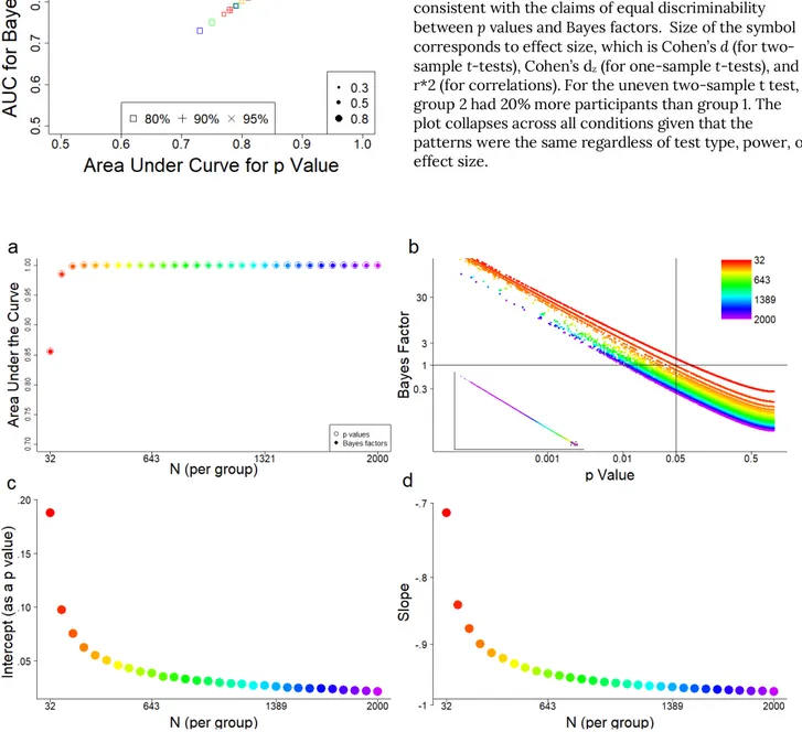
here, Bayes factors are not any better (or worse) than p values at discriminating real effects from null effects. In other words, Bayes factor incurs no advantage over p values at detecting a real effect versus a null effect for the current scenario. This is because Bayes factors are redundant with p values for a given sample size. Both p values and Bayes factors can be calculated from the t-statistic and the sample size, so it is expected that they would be related. In these simulations, there was a near-perfect linear relationship between the (log of the) Bayes factors and the (log of the) p values, as has been shown previously (Benjamin et al., 2017; Krueger & Heck, 2018; Wetzels et al., 2011). Equivalency in AUCs between Bayes factors and p values generalized to other scenarios as well including one-sample t-tests and correlations (see Figure 8).

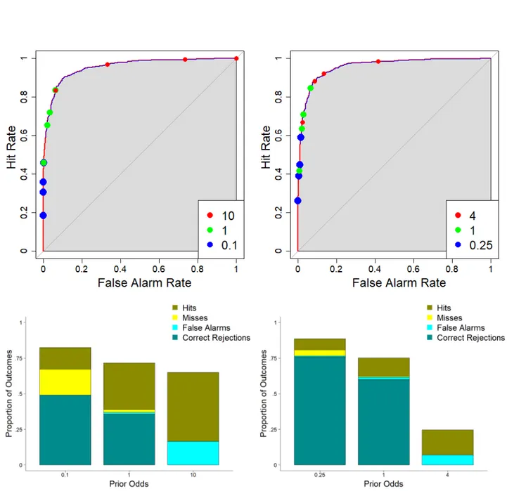
Although the discriminability between p values and Bayes factors was equivalent across a variety of situations, as revealed by equal AUCs (see Figures 2, 8, and 9), the exact relationship between them differed as a function of sample size. In Experiment 6, for 30 different sample sizes ranging from 32 to 2000 per group, 100 simulations of 20 studies were conducted (10 with a Cohen’s d modeled at .50 and 10 with a Cohen’s d modeled at 0). For each sample size, a linear regression was conducted to predict the log of the Bayes factor from the log of the p value. The results are shown in Figure 9. These simulations show near-complete redundancy between p values and Bayes factors. This redundancy also supports the conclusion that for the conditions simulated, p values and Bayes factors are equally adept at distinguishing real effects from null effects.

(10)

WITT

10

Figure 8. Simulations were run for 20 studies (repeated

100 times) for 3 effect sizes for 3 power levels (two-tailed at alpha = .05) for 4 types of statistical tests. AUCs for the Bayes factors are plotted as a function of AUCs for the p values. They are identical in every case, which is consistent with the claims of equal discriminability between p values and Bayes factors. Size of the symbol corresponds to effect size, which is Cohen’s d (for two-sample t-tests), Cohen’s dz (for one-sample t-tests), and

r*2 (for correlations). For the uneven two-sample t test, group 2 had 20% more participants than group 1. The plot collapses across all conditions given that the

patterns were the same regardless of test type, power, or effect size.

Figure 9. Outcomes from 100 simulations of 20 studies (half simulated as a null effect; half as a medium effect) for each

of 30 different sample sizes ranging from 32 to 2000. Color corresponds to sample size. Panel a shows the area under the curve (AUC) for p values and Bayes factors as a function of sample size. A bigger AUC indicates better discrimination between real and null effects. Panel b shows the relationship between p value and Bayes in the range for which p values are highest (the inset shows the relationship for the entire range, and the dotted box shows the area that has been expanded in the main figure). The legend corresponds to sample size. The black vertical line corresponds to a p value of .05, and the black horizontal line corresponds to a Bayes factor of 1. Panels c and d show the intercepts and slopes from linear regressions that predict the log of the Bayes factor from the log of the p values. The intercept is the p value that corresponds to a Bayes factor of 1, so it corresponds to the value of the p value along the horizontal line in panel b. The slope, plotted in panel d, corresponds to the steepness of the curves in panel b

(11)

Figure 10. Left column shows results from Experiment 7 (equal number of null and real effects) and right column shows

results from Experiment 8 (four times as many null as real effects). In the top row, hit rates are plotted as a function of false alarm rates and criterion for Experiment 7 (left panel) and Experiment 8 (right panel). Each point corresponds to a different decision criterion related to the posterior odds (BF > 1, 2, 3, and 10, not labeled but for each cluster of 4, the points go sequentially from top-right corner to bottom-left corner) as a function of the prior odds (see legend). The receiver operator characteristic (ROC) curves are plotted for three different sets of prior odds for each panel. The area under the curve (AUC) is shown in grey. The curves and AUCs are identical across all prior odds in each panel. In the bottom row, proportion of each outcome (calculated as the number of each outcome divided by the total number of studies) across prior odds is shown only for the decision criterion of Bayes factor > 3.

(12)

Despite equivalence in discriminability between

p values and Bayes factor, these simulations

illustrate a previously acknowledged discrepancy in the conclusions supported by the two types of criteria (Lindley, 1957). Specifically, in Figure 9b, all data points to the left of the black vertical line that are also below the black horizontal line would be classified as significant according to the criterion of p < .05 but according to a Bayes factor interpretation, the evidence would favor the null hypothesis over the alternative.

This illustrates why it is possible to get results for which the p value indicates a significant finding (i.e. evidence for the alternative hypothesis) but the Bayes factor shows evidence for the null hypothesis relative to the alternative. These conflicting outcomes occurred in studies for which sample size (or, more precisely, power) was high. These simulations help illustrate the point that for high-powered studies, a p value of .05 is more evidence for the null hypothesis than for the alternative hypothesis (Lakens, 2015). When power is high, researchers using p values to determine statistical significance should use a lower criterion

Including Priors

Whereas Bayes factors do not take into account the prior odds of an effect being real, the posterior odds do. Posterior odds can be calculated by multiplying the Bayes factor by the prior odds (see Equation 1). Posterior odds are the probability of the alternative hypothesis (M = H1) given the data (D) over the null hypothesis (M = H0) given the data (D). To evaluate the effect of prior odds on discriminability, two additional experiments were conducted. In Experiment 7, the same conditions as in Experiment 1 were simulated, but AUCs were calculated for posterior odds across three different prior odds: 0.1, 1, and 10.

Equation 1.

In Experiment 8, everything was the same as in Experiment 1 except there were four times as many studies with d = 0 (16 studies) than with d = .5 (4 studies). AUCs were calculated for posterior odds across three prior odds (.25, 1, 4). As shown in Figure 10, adding information about prior odds to the Bayes factor merely shifted the points along the ROC curve but did not alter discriminability regardless of the accuracy of the prior odds. In addition, changing the proportion of real effects did not have much impact on discriminability. In Experiment 8, the mean AUC was .95 (median = .97, SD = .07) for all sets of prior odds (as well as for p values), which was similar to the mean AUC of .96 (median = .98, SD = .04) for all sets of prior odds (and for p values) in Experiment 7. Except for Experiment 7, all of the simulations conducted involved simulating studies for which half had a true effect and half had a null effect. This assumes that effects are to be expected half of the time, which is an assumption that is unlikely to be true. The results from Experiment 7 show, however, that similar patterns are found even when the null hypothesis is likely to be true. Unreported simulations show similar patterns even when the alternative hypothesis is likely to be true. Thus, the results regarding discriminability (measured with AUCs) are independent of specific assumptions regarding the likelihood of the null hypothesis. Put another way, the discriminability of p values and Bayes factors are high in situations for which real effects are likely and in situations for which real effects are unlikely. Obviously, more p values and Bayes factors reach thresholds for significance when there are more significant effects, so “significant” effects are more for ‘safe’ studies than ‘risky’ studies (Krueger & Heck, 2018). Nevertheless, the diagnosticity of the p value (and of Bayes factor) is high regardless of the likelihood of finding a real effect.

(13)

Bayes Factor and Bias

As with p values, we can consider bias related to Bayes factors. As shown in Figure 3, the cut-offs that achieved maximize utility assuming equal weights given to false alarms and misses was Bayes factor > 1. This contrasts with the typical interpretation of Bayes factor (e.g., Table 2) for which Bayes factors between 1-3 are considered anecdotal evidence.

Unlike with p values, the threshold that should be used for Bayes factors did not vary as much with changes in sample size as did the alpha levels of the

p values (see Figure 10). Compare the red points to

the green points, which correspond to p < .10 and p < .005. For smaller sample sizes, the red points achieve better performance than the green points, but for larger sample sizes, the relationship flips and the green points achieve better performance. This repeats the point made earlier that at larger sample sizes, a lower alpha should be used. For Bayes factors, compare the light blue and purple points, which correspond to Bayes factor thresholds of 1 and 3. For smaller sample sizes, the light blue points achieved better performance, but for larger sample sizes, the purple points achieved better performance. However, unlike with p values, this reversal was not nearly as dramatic, and the decision criterion of Bayes factor > 1 performed better than or nearly as good as the other thresholds across all sample sizes. It is also worth noting that as sample size increases, all Bayes factor criteria improved, whereas p values plateaued at their alpha levels. Thus, another advantage of Bayes factors is that increasing the amount of evidence increases their ability to accurately detect an effect.

Signal detection analysis is a tool that scientists can use to evaluate relative trade-offs across various decision criteria. This is not to say that scientists should only use or always use decision criteria (as opposed to estimations of effect size, for example), but that when a criterion for statistical significance

is adopted, consideration should be made for both false alarms and misses. If the goal is to maximize optimal utility, given equal weight to hits and correct rejections (or, equivalently, equal tolerance for false alarms and misses), distance to perfection can be used to assess various criteria. In the case of a medium effect size

with 64 participants per group, the decision criteria of p < .10, p < .05, and BF > 1 led to better performance than the criteria of p < .005, BF > 3, and BF > 10. As sample size increased, the criteria of p < .005 and all tested Bayes factor thresholds led to better performance than p < .10.

Discriminability with Effect Size

As a final note, discriminability (as measured using AUCs) was as good or better when using effect size (in this case, Cohen’s d) than p values or Bayes factors (see Figure 14). Effect size improved discriminability because Cohen’s d is signed (i.e. differentiates -.5 from .5). When discriminability was assessed using absolute effect size, the AUCs matched those obtained with p values and Bayes factors. The measure of effect size does not have the feature of a specific decision criterion for statistical significance, so for researchers who want strict thresholds for significance, effect size is unlikely to be a useful tool. But for researchers who want to know the strength of the evidence or the magnitude of the effect, effect size would be useful.

(14)

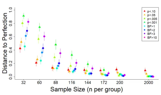
Figure 11. Distance to perfection was calculated as the Euclidean distance between each point on the ROC curve (see

Figure 2) and the top-left corner (which corresponds to 100% hit rate and 0% false alarm rate). Distance to perfection scores were calculated for each of 100 sets of 20 studies (half of which were modeled as a null effect and half of which were modeled with Cohen’s d = .5) for each sample size. The data are grouped by sample size, and color corresponds to the criterion for statistical significance. Errors bars correspond to 95% confidence intervals.

Figure 12. Area under the curve (AUC) for Cohen’s d as a

function of the AUCs for p values and Bayes factors (BF). Data are from Experiment 1. Each point corresponds to one set of 20 studies with half modeled with Cohen’s d = .5 and half modeled with Cohen’s d = 0. Dotted line is at unity.

Conclusion

An essential part of science is that it is replicable. But another essential part of science is to uncover new discoveries. Changing the standard criterion for statistical significance merely moves the standard along the ROC curve. Any change to this standard such as decreasing the required p value or using Bayes factors instead will not improve discriminability between real and null effects. Rather, a change to be more conservative will decrease false alarm rates at the expense of increasing miss rates. False alarm rates should not be considered in isolation without also considering miss rates. Rather, researchers should consider the relative importance for each in deciding the criterion to adopt. This aligns with other recommendations for researchers to justify their alphas (Lakens et al., 2018). In addition, given that true null results can be theoretically interesting and practically important, a conservative criterion can produce critically misleading interpretations by labeling real effects as if they were null effects.

(15)

Moving forward, the recommendation is to acknowledge the relationship between false alarms and misses, rather than implement standards based solely on false alarm rates.

Open Science Practices

This article earned the Open Materials badge for making the materials available. It has been verified that the analysis reproduced the results presented in the article. The entire editorial process, including the open reviews, are published in the online supplement.

References Begley, C. G., & Ellis, L. M. (2012). Drug

development: Raise standards for preclinical cancer research. Nature, 483(29 March), 531-533. doi: 10.1038/483531a

Benjamin, D. J., Berger, J. O., Johannesson, M., Nosek, B. A., Wagenmakers, E. J., Berk, R., . . . Johnson, V. E. (2017). Redefine statistical significance. Nature Human Behaviour. doi: 10.1038/s41562-017-0189-z

Camerer, C. F., Dreber, A., Forsell, E., Ho, T.-H., Huber, J., Johannesson, M., . . . Wu, H. (2016). Evaluating replicability of laboratory

experiments in economics. Science, 351(6280), 1433-1436.

Collaboration, O. S. (2015). Estimating the reproducibility of psychological science.

Science, 349(6251), aac4716. doi:

10.1126/science.aac4716

Dienes, Z. (2011). Bayesian versus orthodox

statistics: Which side are you on? Perspectives

on Psychological Science, 6, 274-290. doi:

10.1177/1745691611406920

Etz, A., & Vandekerckhove, J. (2016). A Bayesian perspective on the reproducibility project: Psychology. PLos One, 11(2), e0149794. doi: 10.1371/journal.pone.0149794

Fiedler, K., Kutzner, F., & Krueger, J. I. (2012). The Long Way From α-Error Control to Validity Proper: Problems With a Short-Sighted False-Positive Debate. Perspectives on Psychological

Science, 7(6), 661-669. doi:

10.1177/1745691612462587

Fraley, R. C., & Vazire, S. (2014). The N-Pact Factor: Evaluating the Quality of Empirical Journals with Respect to Sample Size and Statistical Power. PLOS ONE, 9(10), e109019. doi: 10.1371/journal.pone.0109019

Green, D. M., & Swets, J. A. (1966). Signal Detection

Theory and Psychophysics. New York: Wiley.

Ioannidis, J. P. A. (2005). Why most published research findings are false. PLoS Med, 2(8), e124. doi: 10.1371/journal.pmed.0020124

Jeffreys, H. (1961). Theory of Probability. Oxford, UK: Oxford University Press.

Kass, R. E., & Raftery, A. E. (1995). Bayes factors.

Journal of the American Statistical Association, 90(430), 773-795.

Krueger, J. I., & Heck, P. R. (2017). The Heuristic Value of p in Inductive Statistical Inference.

Frontiers in Psychology, 8(908). doi:

10.3389/fpsyg.2017.00908

Krueger, J. I., & Heck, P. R. (2018). Testing

significance testing. Collabra: Psychology, 4(1), 11. doi: 10.1525/collabra.108

Kruschke, J. K. (2013). Bayesian estimation

supersedes the t test. Journal of Experimental

Psychology: General, 142(2), 573-603. doi:

10.1037/a0029146

Lakens, D. (2014). Performing high-powered studies efficiently with sequential analyses. European

Journal of Social Psychology, 44, 701-710. doi:

10.1002/ejsp.2023

Lakens, D. (2015, March 20, 2015). How a p-value between 0.04-0.05 equals a p-value between 0.16-017. Retrieved from

http://daniellakens.blogspot.com/2015/03/h ow-p-value-between-004-005-equals-p.html Lakens, D. (2016, 1/14/16). Power analysis for

default Bayesian t-tests. Retrieved from http://daniellakens.blogspot.com/2016/01/p ower-analysis-for-default-bayesian-t.html Lakens, D., Adolfi, F. G., Albers, C. J., Anvari, F.,

Apps, M. A. J., Argamon, S. E., . . . Zwaan, R. A. (2018). Justify your alpha. Nature Human

(16)

WITT

16

Behaviour, 2(3), 168-171. doi:

10.1038/s41562-018-0311-x

Lee, M. D., & Wagenmakers, E. J. (2005). Bayesian statistical inference in psychology: Comment on Trafimow (2003). Psychological Review,

112(3), 662-668. doi:

10.1037/0033-295X.112.3.662

Lindley, D. V. (1957). A statistical paradox.

Biometrika, 44(1/2), 187-192.

Macmillan, N. A., & Creelman, C. D. (2008).

Detection Theory: A User's Guide (Second Edition). New York: Psychology Press.

McShane, B. B., Gal, D., Gelman, A., Robert, C., & Tackett, J. L. (2018). Abandon statistical significance. arXiv preprint. doi: arxiv.org/pdf/1709.07588

Morey, R. D. (2015, 5/31/18). On verbal categories for the interpretation of Bayes factors Retrieved from

http://bayesfactor.blogspot.com/2015/01/on -verbal-categories-for-interpretation.html Morey, R. D., Rouder, J. N., & Jamil, T. (2014).

BayesFactor: Computation of Bayes factors for common designs (Version 0.9.8), from

http://CRAN.R-project.org/package=BayesFactor Murayama, K., Pekrun, R., & Fiedler, K. (2014).

Research Practices That Can Prevent an Inflation of False-Positive Rates. Personality

and Social Psychology Review, 18(2), 107-118. doi:

10.1177/1088868313496330

Rouder, J. N., Speckman, P. L., Sun, D., Morey, R. D., & Iverson, G. (2009). Bayesian t-tests for accepting and rejecting the null hypothesis.

Psychonomic Bulletin & Review, 16, 225-237. doi:

10.3758/PBR.16.2.225

Salomon, E. (2015). P-Hacking True Effects. Retrieved from

http://www.erikasalomon.com/2015/06/p-hacking-true-effects/

Schönbrodt, F. D., & Wagenmakers, E.-J. (2018). Bayes factor design analysis: Planning for compelling evidence. Psychonomic Bulletin &

Review, 25(1), 128-142. doi:

10.3758/s13423-017-1230-y

Sedlmeier, P., & Gigerenzer, G. (1989). Do studies of statistical power have an effect on the power of studies? Psychological Bulletin, 105(2), 309-316. doi: 10.1037/0033-2909.105.2.309

Simmons, J. P., Nelson, L. D., & Simonsohn, U. (2011). False-positive psychology: Undisclosed

flexibility in data collection and analysis allows presenting anything as significant.

Psychological Science, 22(11), 1359-1366. doi:

10.1177/0956797611417632

Team, R. C. (2017). R: A language and environment for statistical computing. Retrieved from https://www.r-project.org

Trafimow, D., & Marks, M. (2015). Editorial. Basic

and Applied Social Psychology, 37(1), 1-2.

Wetzels, R., Matzke, D., Lee, M. D., Rouder, J. N., Iverson, G. J., & Wagenmakers, E.-J. (2011). Statistical evidence in experimental

psychology: An empirical comparison using 855 t tests. Perspectives on Psychological Science,