2016:23 Technical Note, Modelling of the thermal evolution of the KBS-3 repository at Forsmark and associated induced seismic activity

(1)

Technical Note

Modelling of the thermal evolution of

the KBS-3 repository at Forsmark and

associated induced seismic activity

Main Review Phase

2016:23

Authors: Jeoung Seok Yoon

Ove Stephansson Ki-Bok Min

(2)

(3)

SSM perspektiv

Bakgrund

Strålsäkerhetsmyndigheten (SSM) granskar Svensk

Kärnbränslehanter-ing AB:s (SKB) ansöknKärnbränslehanter-ingar enligt lagen (1984:3) om kärnteknisk

verk-samhet om uppförande, innehav och drift av ett slutförvar för använt

kärnbränsle och av en inkapslingsanläggning. Som en del i granskningen

ger SSM konsulter uppdrag för att inhämta information och göra

expert-bedömningar i avgränsade frågor. I SSM:s Technical Note-serie

rap-porteras resultaten från dessa konsultuppdrag.

Projektets syfte

Det övergripande syftet med projektet är att ta fram synpunkter på

SKB:s säkerhetsanalys SR-Site för den långsiktiga strålsäkerheten för det

planerade slutförvaret i Forsmark. Innehållet i denna rapport redovisar

resultaten från modellering av den termiska utvecklingen i slutförvaret

och den seismiska aktivitet som kan uppkomma i samband med värmen

som det utbrända kärnbränslet alstrar. I rapporten redovisas också

resul-taten från modellering av skjuvdeformationer hos sprickor som

förekom-mer i berget för slutförvaret till följd av att ett jordskalv bildas i någon av

de större deformationszonerna i slutförvarets omedelbara närhet under

den tid som värmen alstras av utbrända kärnbränslet.

Författarnas sammanfattning

Denna studie redovisar flera förlopp som kan påverka den fysiska

integ-riteten hos ett slutförvar av utbränt kärnbränsle i Forsmak. Två möjliga

skäl till detta är: i) den värme som det utbrända kärnbränsle i kapslarna

som avklingar med tiden alstrar och som värmer upp berget, och ii)

jord-skalv som bildas hos någon av de större deformationszoner som finns

i slutförvarets omedelbara närhet samtidigt som värme alstras av det

utbrända kärnbränslet.

Av speciell vikt för säkerheten är skjuvdeformationen hos existerande

sprickor i slutförvaret som kan uppkomma i samband med

värmelas-ten från utbrända bränslet eller skjuvdeformationen som effekt av ett

jordskalv som bildas hos någon av deformationszonerna i närheten av

slutförvaret eller en kombination av dessa bägge. I SKB:s säkerhetsanalys

SR-Site redovisas en största tillåten skjuvdeformation om 50 mm för en

bergspricka som förekommer i deponeringshålet för kapseln eller dess

omedelbara närhet.

Den termiska belastningen och simuleringen av jordskalv i denna

studie har utförts med den tvådimensionella beräkningskoden PFC2D

som baseras på diskreta elementmetoden DEM. Beräkningsmodellen

simulerar explicita deformationszoner och spricknät som finns i

Fors-marksområdet samt för de olika paneler som slutförvaret består av som

SKB redovisat. I modellerna simuleras värmelasten som punktkällor.

Tvådimensionella horisontal- och vertikalsektioner av slutförvaret har

simulerats i denna studie. Ett jordskalv som simuleras i beräkningarna

(4)

alstras genom en momentan frigörelse av den töjningsenergi som

bergspänning arna alstrat och som lagrats hos de många små sprickor

(smooth joints) som deformationszonen består av.

Från simuleringen av värmelastens respons hos sprickorna i slutförvaret

visar resultaten att skjuvdeformationerna ökar när temperaturen i

berg-massan ökar. Resultaten från PFC2D- simuleringen visar att för såväl en

momentan deponering av samtliga kapslar i slutförvaret och för det fall

deponeringen sker under en tidsperiod av ca 100 år så överskrids i intet

fall deformationsvillkoret 50 mm.

Från samtidig modelleringen av värmelasten och simuleringen av ett

jordskalv vid rådande spänningstillstånd i berget visar resultaten från

PFC2D-simuleringen av ett jordskalv med magnituden på upp till Mw4.7

på någon av deformationszonerna ZFMMWNW0809A (i

horisontalsek-tionen) respektive deformationszon ZFMA3 (i vertikalsekhorisontalsek-tionen) 100 år

efter deponeringen har avslutats leder till att ingen spricka i slutförvaret

överskrider gränsvärdet för skjuvdeformationen på 50 mm.

Från en tolkning av modelleringsresultaten där man tar i beaktande de

möjliga felkällorna hos beräkningskoden, drar författarna slutsatsen att

risken för kapselbrott till följd av värmelasten samt värmelasten i

kombi-nation med ett jordskalv vid dagens förhållanden är mycket osannolik.

Projektinformation

Kontaktperson på SSM: Flavio Lanaro

Diarienummer ramavtal: SSM2011-3631

Diarienummer avrop: SSM2013-3839

Aktivitetsnummer: 3030012-4077

(5)

SSM perspective

Background

The Swedish Radiation Safety Authority (SSM) reviews the Swedish

Nuclear Fuel Company’s (SKB) applications under the Act on Nuclear

Activities (SFS 1984:3) for the construction and operation of a

reposi-tory for spent nuclear fuel and for an encapsulation facility. As part of

the review, SSM commissions consultants to carry out work in order to

obtain information and provide expert opinion on specific issues. The

results from the consultants’ tasks are reported in SSM’s Technical Note

series.

Objectives of the project

The general objective of the project is to provide review comments on

SKB’s post-closure safety analysis, SR-Site, for the proposed repository

at Forsmark. In particular, this assignment concerns the development

of shear displacements of the repository target fractures induced by the

heat that is generated from the disposed canisters containing the spent

nuclear fuel. This assignment also concerns the shear displacements of

the repository target fractures induced by an earthquake at a nearby

deformation zone occurring while the repository is under heat loading.

Summary by the authors

This study addresses several events that could impair the physical

integrity of the repository of spent nuclear fuel at the Forsmark site. Two

sources of threat are: i) events due to thermal loading on the rock mass

by the heat from canisters with spent nuclear fuel, and ii) seismic events,

i.e. earthquakes, at the nearby deformation zones that occur during the

time when the repository is under heat loading.

The effect relevant to the repository safety is the shear displacement on

rock fracture induced either by the effect of thermal loading, or by an

earthquake at a nearby deformation zone, or by the combination of the

two. In SKB’s safety assessment SR-Site, a shear displacement of 50 mm

of a target fracture that crosses a canister position in the repository is

regarded as the upper limit of canister damage.

Thermal loading and earthquake simulations in this study are

con-ducted using PFC2D, a 2-D discrete element code (DEM). The PFC2D

models include a large number of explicitly modelled deformation zones,

target fractures and point-heat sources arranged into deposition panels

as reported by SKB. Horizontal and vertical cross-sections of the

reposi-tory are considered in this study.

Earthquake at a specific deformation zone is simulated by a sudden

release of the strain energy that was accumulated under the given

present-day stress conditions and stored in smaller fractures building up

the deformation zones.

From the modelling of heat induced fracture responses, it is observed

that the shear displacement of the repository target fractures increase

(6)

when the temperature in the rock mass increases. Taking into account of

the possible numerical artefacts of PFC2D and outliers in the results, in

both modelling cases where the canisters are disposed simultaneously

and sequentially, canister damage by the shear of the target fractures

due to heat loading is very unlikely.

From the modelling of heat and earthquake induced fracture responses

under present-day stress conditions at Forsmark, it is found that for an

earthquake with moment magnitude up to Mw4.7 at deformation zones

ZFMWNW0809A (horizontal section) and ZFMA3 (vertical section) that

occur 100 year after completion of simultaneous deposition, there are

no fractures experiencing shear displacements larger than the canister

damage threshold of 50 mm.

From the interpretation of the modelling results with full consideration

of the possible effects of the numerical artefacts in PFC2D, the Authors

draw a conclusion that a risk of canister damage due to the heat

load-ing or the combined loadload-ing of heat and the earthquake in present-day

conditions is very unlikely.

Project information

(7)

2016:23

Authors: Jeoung Seok Yoon 1)_{, Ove Stephansson}2)

1)_{Stephansson Rock Consultant, Berlin, Germany} 2)_{Seoul National University, Seoul, Republic of Korea}

Modelling of the thermal evolution of

the KBS-3 repository at Forsmark and

associated induced seismic activity

Main Review Phase

(8)

This report was commissioned by the Swedish Radiation Safety Authority

(SSM). The conclusions and viewpoints presented in the report are those

of the author(s) and do not necessarily coincide with those of SSM.

(9)

1. Introduction

The Swedish Radiation Safety Authority (SSM) reviews the Swedish Nuclear Fuel Company’s (SKB) applications under the Act on Nuclear Activities (SFS 1984:3) for the construction and operation of the KBS-3 repository for spent nuclear fuel and for an encapsulation facility. As part of the review, SSM commissions consultants to carry out work in order to obtain information and provide expert opinions on specific scientific and technical issues. The results from the consultants’ tasks are reported in SSM’s Technical Note series.

The general objective of the review is to provide comments on SKB’s post-closure safety analysis, SR-Site (SKB, 2011), for the proposed repository at Forsmark, Sweden. In particular, this assignment concerns the development of the shear displacement along repository fractures induced by the heat that is generated by the disposed canisters containing the spent nuclear fuel. This assignment also concerns the shear displacement of the repository fractures induced by an earthquake at a nearby deformation zone occurring while the repository is under heat loading from the disposed canisters.

This Technical Note is complementary to SSM Technical Note 2014:59 entitled “Relation between earthquake magnitude, fracture length and fracture shear displacement in the KBS-3 repository at Forsmark – Main Review Phase” (Yoon et al., 2014).

1.1. Background

Yoon et al. (2014) have conducted numerical modelling studies that analyse the shear displacement of the repository fractures (also called “target fractures”) induced by the heat generated from the disposed canisters containing the spent nuclear fuel and/or by a seismic loading generated by earthquakes occurring at nearby large deformation zones. The heat sources in the thermo-mechanical coupled analyses in Yoon et al. (2014) were modelled similarly to the methods used in a few other SSM reports (Backers and Stephansson, 2011; Ofoegbu and Smart, 2013; Backers et al. 2014), which used the output temperature of SKB’s 3DEC modelling results as an input to their modelling. Furthermore, the rock mass temperature in Yoon et al. (2014) was instantaneously increased from 11.2°C to 50°C. Such instantaneous increase of temperature over an area of a few square kilometres caused large thermal shocks to the repository rock mass, and consequently resulted in thermally induced seismic events of relatively large magnitude. The concern that Yoon et al. (2014) might have overestimated the fracture responses led to development of the present assignment where the shear displacement on rock fractures in the numerical model is verified against analytical solutions and results from other numerical codes.

Furthermore, thermo-mechanical coupled modelling of the KBS-3 repository is conducted by considering more realistic heat emission curves from the canisters and the effect of possible numerical artefacts in PFC2D discrete element modelling are studied.

(12)

1.2. Assigned topics

The following tasks are conducted in this study:

 Task A: Verification of the modelling method with PFC2D, in particular

reliability of the calculation of fracture shear displacements,

 Task B: Modelling of thermally induced shear displacements of the

repository target fractures, distribution of induced seismic events and their magnitudes in the horizontal and vertical sections of the repository,

 Task C: Modelling of earthquake induced shear displacements of the

repository target fractures, distribution of induced seismic events during operational and thermal phase of the repository.

Task A’s verification of the calculations of fracture shear displacement is covered in Chapter 2.

Task B’s analyses of target fracture responses due to thermal loading induced by the heat from the spent nuclear fuel for the horizontal and vertical sections of the repository are covered in Chapters 3, 4 and 5.

Task C’s analysis of target fracture responses induced by a tectonic earthquake at a nearby major deformation zone hits the repository during the operational and thermal phase of the repository due to the heat generated by the spent nuclear fuel for the horizontal and vertical sections of the repository is covered in Chapter 6. General considerations on the modelling results and their implications for the safety of the repository are covered in Chapter 7.

1.3. Description of the Appendices

This report contains five Appendices that contain the following:

 Appendix A lists SKB reports that were reviewed for this assignment,

 Appendix B presents close-up views of the parts of the model with fracture

intersections. The model is used for verification of the fracture shear displacements covered in Chapter 2.

 Appendix C lists the results of the modelling with FRACOD2D of fracture

shear displacements to be compared with the modelling results with PFC2D in Chapter 2.

 Appendix D discusses the results of the heat conduction modelling using

COMSOL.

(13)

2. Analysis of fracture shear

displacements with PFC2D

In this Chapter, we investigate the shear displacement of a fracture that consists of many smooth joints (Mas Ivars et al., 2011), a so called “PFC fracture”, and embedded in an elastic continuum volume. The objective of this investigation is to study if the shear displacement of a single PFC fracture shows the parabolic profile along its trace when subjected to shear stress.

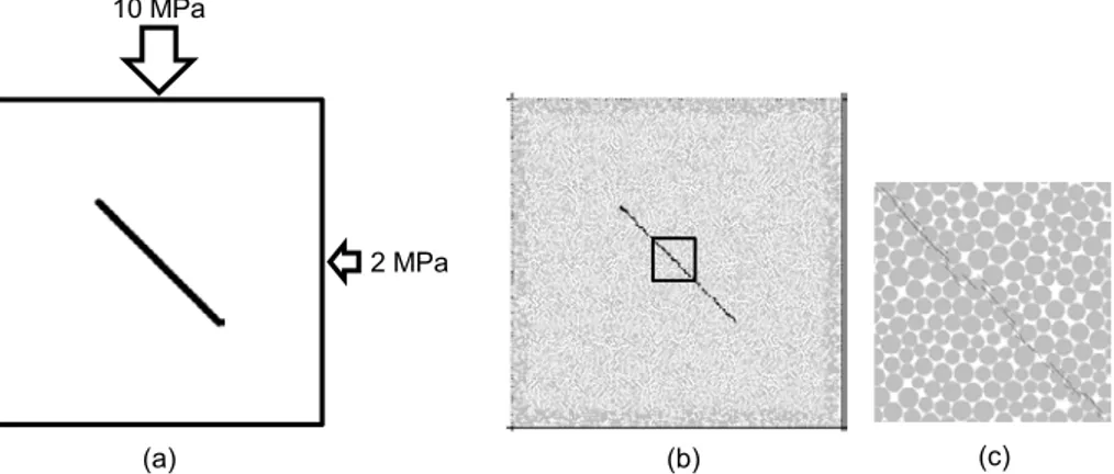
For the verification tests, we use a two-dimensional rectangular model with size of 2 km by 2 km as shown in Figure 1 that contains an inclined and isolated PFC fracture with 500 m half-length and subjected to an anisotropic stress field.

Figure 1. (a) Schematics of the verification test model containing an inclined and isolated fracture subjected to shear loading, (b) realization in PFC2D using smooth joints, and (c) enlarged view of the box area in (b) showing a detail of the PFC particles and smooth joints.

2.1. Comparison with an analytical solution

According to Pollard and Segall (1987), the shear displacement at an arbitrary position within a fracture can be calculated in 2D using the following equation:

√ Eq. (1)

where τr is the remote shear stress, τc is the shear stress on the fracture, v is the

Poisson’s ratio and G is the shear modulus of the rock, a is the fracture half length, and r is the distance of the occurrence point of the shear displacement from the fracture centre. In the example in Figure 2, ∆τ is 4 MPa and the friction angle and cohesion of the fracture are assumed to be zero.

Shear displacement of the smooth joints in the PFC2D model are plotted with respect to their distance from the fracture centre and compared in Figure 2 with the analytical solution of Equation (1). The Young’s modulus E and the Poisson’s ratio

v of the particle assembly block can be obtained by the uniaxial compression 10 MPa

2 MPa

(14)

simulation, and are chosen in range between 59 GPa to 70 GPa and in range between 0.23 to 0.28, respectively. These properties match well with those of the dominant rock type at Forsmark. The shear modulus G is calculated by the equation

G = E/2(1+v). The smooth joint friction coefficient μ is set to zero. The simulated

shear displacements of the smooth joints with PFC2D show a good match with the analytical solution.

Equation (2) is a 3D version of Equation (1) and gives the shear displacement at a distance r from the centre of a circular fracture of radius a:

√ Eq. (2)

Figure 2. Comparison between the shear displacement profile of a PFC fracture and the analytical solution by Pollard and Segall (1987) (Eq.1).

2.2. Effect of friction and length of the fractures

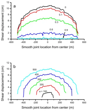
This test is intended to investigate how the friction coefficient of the smooth joints affects the shear displacement distribution of a PFC fracture. The bond strength of the smooth joints is set to zero so that the smooth joints of the PFC fracture can slide at the onset of applying shear stress. Five cases of smooth joint friction coefficients (0, 0.1, 0.3, 0.6 and 0.9) are tested and the results are shown in Figure 3a. The results show that the lower the friction of the smooth joints the larger the displacement of the fracture.

The second test investigates how dependent the fracture displacement is on the fracture length in the PFC2D model. In this test, the length of the fracture is varied (half length a = 100, 200, 300, 400 and 500 m) while the friction coefficient μ is set to 0.1. The results show that the larger the fracture the larger the shear displacement (Figure 3b). The results indicate that the proportionality between the fracture length and the fracture displacement is confirmed by the PFC2D modelling.

-600 -400 -200 0 200 400 600 0 2 4 6 8 10 12 PFC2D (a = 500 m,  = 0)

analytical (E=70 GPa; v=0.23)

Shear displacement

(cm)

(15)

Figure 3. Effect of (a) friction coefficients μ and (b) fracture length 2a on the shear displacements of the smooth joints of the PFC fractures.

2.3. Effect of intersecting fractures

This test is intended to investigate if the parabolic profile of shear displacement of a PFC fracture holds when multiple PFC fractures are intersecting each other. Three cases are tested: (i) one PFC fracture, (ii) two intersecting PFC fractures, and (iii) five intersecting PFC fractures (Figure 4). The applied principal stresses are the same as in the two previous tests. Figure 5 shows the shear displacement of smooth joints after normalization against the maximum shear displacement in each of the PFC fractures (in red: the largest displacement, green: the smallest displacement, see the colour scale on the left side of Figure 5a). Along the traces of the PFC fractures, we present the absolute shear displacements of the smooth joints in the right column of Figure 5. The figure shows that the parabolic profiles are broken when PFC fractures are intersected by other fractures also under shear. Especially, there is a sudden jump/drop of the displacement at the location of fracture intersection (Figure 5b). The displacement profiles become more complex when there are more fractures intersecting: this is evident when comparing the red curves in Figure 5b and Figure 5c. The intersection between Fracture #3 and #4 in Figure 5c shows one smooth joint with very high shear displacement compared to the others. The particle displacement field near that area of fracture intersection is shown in Figure 6, which indicates that the displacement is localized at one specific particle located at the corner of the two fractures (black arrow). Due to this localized displacement at the particle, the smooth joints attached to the particle undergo relatively large shear displacements compared to other neighbouring smooth joints, also addressed as “spikes” of the fracture shear displacement profiles. The smooth joints are coloured according to 10-based logarithm of the shear displacement.

-600 -400 -200 0 200 400 600 0 2 4 6 8 10 12 Shear dis plac ement (c m)

Smooth joint location from center (m)

-600 -400 -200 0 200 400 600 0 2 4 6 8 10 12 0.9 0.6 0.3 0.1 0 Shear dis plac ement (c m)

Smooth joint location from center (m)

a b a = 100 200 300 400 500

(16)

Appendix B provides close-up views on all seven fracture intersections.

Figure 4. PFC2D models containing (a) one PFC fracture, (b) two intersecting PFC fractures, and (c) five intersecting PFC fractures.

Figure 5. Distribution of shear displacement of the smooth joints of (a) one PFC fracture, (b) two intersecting PFC fractures, (c) five intersecting PFC fractures, and their absolute displacement distributions along the traces.

a b c -1000 -500 0 500 1000 -1000 -500 0 500 1000 0 10.00 20.00 30.00 40.00 50.00 60.00 70.00 80.00 90.00 100.0 -1000 -500 0 500 1000 -1000 -500 0 500 1000 2 1 -1000 -500 0 500 1000 -1000 -500 0 500 1000 5 4 3 2 1 a b c -600 -400 -200 0 200 400 600 0 5 10 15 20 25

Distance from center (m)

Shear dis plac ement (c m) -600 -400 -200 0 200 400 600 0 5 10 15 20 25

1 2 Shear dis plac ement (c m) -600 -400 -200 0 200 400 600 0 5 10 15 20 25 1 2 3 4 5 Shear dis plac ement (c m)

(17)

Figure 6. (Left) Close-up view of the intersection 6 between Fracture #3 and #4 in the PFC2D model (smooth joints in red and particle displacement with a black arrow). (Right) The smooth joints are coloured according to 10-based logarithm of the shear displacements.

2.4. Effect of fracture insertion order

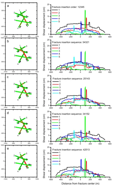
This test is intended to investigate the effect of the order of fracture insertion on the fracture shear displacement, i.e. whether the occurrence of spikes in the profile of the shear displacements is dependent on the order in which fractures are inserted. The five fractures shown in Figure 5c are inserted in the model in different orders: 12345, 54321, 25143, 34152 and 42513. Figure 7 shows the shear displacement profiles of the five intersecting PFC fractures that are placed in the model in different orders.

The results show that the occurrence of spikes and their locations along the fracture trace are dependent on the fracture insertion order, and thus on the particular position of some of the smooth joints.

2.5. Effect of particle size

The tests presented in Section 2.4 are repeated on a particle assembly packed with relatively small particles. The tests are intended to investigate the effect of particle size on the shear displacement profile of the fractures. The diameter range of the particle assembly in Section 2.4 is 7 to 22 m, whereas in this section it is chosen to be 5 to11 m for the smaller particle assembly in this section. Figure B-3 in Appendix B shows the shear displacement profiles of the five intersecting PFC fractures that are placed in the smaller particle assembly in different orders. The results show that, irrespective of the fracture insertion order, there are four distinct peaks or spikes of shear displacements at the intersection of Fracture #1 and #3 and at the intersection of Fracture #2 and #5. The particle displacement fields near the area of intersections for the case of fracture insertion order of 12345 are also shown in Appendix B. Compared to the results in Section 2.4, the use of smaller particle does not seem to have significant effect on reducing the peak displacement, but on the opposite, it seems to increase the peak. Shear displacement profiles of other fractures are more or less the same irrespective of the fracture insertion order.

-50 0 50 100 150 -300 -250 -200 -150 -100 x (m) y (m ) -4.000 -3.500 -3.000 -2.500 -2.000 -1.500 -1.000 -0.5000 0 log(Us)

(18)

Figure 7. Shear displacement profiles of five intersecting fractures placed in different orders, (a) 12345, (b) 54321, (c) 25143, (d) 34152 and (e) 42513 in a larger particle assembly.

a b c d e -1000 -500 0 500 1000 -1000 -500 0 500 1000 3 4 2 1 5 -1000 -500 0 500 1000 -1000 -500 0 500 1000 5 4 3 2 1 -1000 -500 0 500 1000 -1000 -500 0 500 1000 3 4 2 1 5 -1000 -500 0 500 1000 -1000 -500 0 500 1000 3 4 2 1 5 -1000 -500 0 500 1000 -1000 -500 0 500 1000 3 4 2 1 5 -600 -400 -200 0 200 400 600 0 5 10 15 20 25

Fracture insertion order: 12345 1 2 3 4 5 Shear dis plac ement (c m)

-600 -400 -200 0 200 400 600 0 5 10 15 20 25

Fracture insertion sequence: 54321 1 2 3 4 5 Shear dis plac ement (c m)

Distance from fracture center (m)

-600 -400 -200 0 200 400 600 0 5 10 15 20 25

(19)

2.6. Effect of “rattler” particles and stress

concentrations at the tips of the fractures

The PFC2D modelling results show that the shear displacement profile of an isolated fracture is in good agreement with the analytical solution. This demonstrates that modelling with PFC2D of shear displacement of a fracture represented by a collection of smooth joints is reliable.

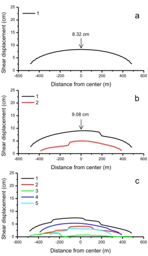
The displacement profile deviates from the parabolic shape when fractures are intersecting. The shear displacement profiles of five intersecting fractures shown in Figure 5 are modelled with FRACOD2D (Shen, 2014) and results are presented in Figure 8. In general, the parabolic shear displacement profile for an isolated fracture is interrupted at the intersection with other fractures. Also as seen in Figure 8a and 8b, the maximum displacement in the models is larger than for an isolated fracture of the same size.

Differently than for the PFC2D results, the results from FRACOD2D show smooth distributions of the displacement along the fractures independently of the

intersections. This is due to the fact that a fracture modelled in FRACOD2D is perfectly linear, whereas a fracture modelled in PFC2D consists of many discrete smooth joints. Nevertheless, for an isolated fracture case, the maximum shear displacement takes place at the centre of the fracture and the calculated magnitudes the same identical for the two models (8.32 cm as in Figure 8a).

For the case with two intersecting fractures, the FRACOD2D results also show a displacement jump at the intersection. However, the displacement profile of Fracture #1 does not show a spike of the displacement as in the PFC2D model in Figure 5b where it reaches about 12 cm.

For the case with five intersecting fractures, the difference between the two modelling results becomes more distinct. The PFC2D results show four distinct displacement spikes at the fracture intersections, whereas the FRACOD2D results show no displacement spikes but only several smaller jumps at the intersections. In summary, the displacement profiles of some of the PFC fractures are showing significantly large of the shear displacement values at the intersections. As there is no closed form solution for calculating shear displacements of intersecting fractures, efforts have been made to investigate if such peak displacements at the intersection areas are physically possible or are only local numerical errors or artefacts produced by PFC2D.

(20)

Figure 8. Shear displacement profiles of (a) single isolated fracture, (b) two intersecting fractures, and (c) five intersecting fractures modelled with FRACOD2D.

From a number of tests, it is found that irrespective of the particle size and the order of fracture insertion, there are always several spikes of the shear displacement at some of the fracture intersections. By the stress analysis in FRACOD2D (see Appendix C) and in PFC2D (see Appendix C, Figures C-10 and C-11), it is confirmed that stresses tend to concentrate at the fracture intersections where the spikes occur.

The stress analysis demonstrates that the spikes of shear displacement at the fracture intersection in PFC2D are due to excessive stress concentration on rigid particles as shown in Figure 6. Localized displacement of one particle leads to concentrated shear displacements of the smooth joints around the particle. This is the reason why significantly large shear displacement spikes occur at the fracture intersections. In reality, however, stress concentrations at the fracture tip or at the fracture

intersection may easily lead to local failure of the rock at that point. If the rock at the location of fracture intersection fails, a localized displacement as it was modelled in PFC2D, i.e. displacement spikes, may not be observed. The failure of the rock near the fracture intersection may dissipate some of the energy concentration. Therefore, in reality, fracture shear displacement at that location would be reduced. But at the same time, the left-over energy after the local failure could go into the neighbouring

-600 -400 -200 0 200 400 600 0 5 10 15 20 25 1 Shear dis plac ement (c m)

-600 -400 -200 0 200 400 600 0 5 10 15 20 25 1 2 3 4 5 Shear displacement (cm)

-600 -400 -200 0 200 400 600 0 5 10 15 20 25 1 2 Shear dis plac ement (c m)

a

b

c

8.32 cm

(21)

space and volume and slightly increase the shear displacement adjacent to the fracture intersection.

Later investigation on this issue has led to further findings namely, that the highly localized displacement on one particle in PFC2D as shown in Figure 6 is due to the fact that the particle detaches from the surrounding particles. For this reason, particles behaving this way are named “rattlers”. The rattler particle occurs due to stress concentration as shown in the stress analysis (see Appendix C) and depends on the fact that the particles in PFC2D are rigid and non-breakable. When high stress concentrations are developed at some smooth joint intersections, the bond strength between the particles can be overcome and the bonds may break. The particle might then lose all bonds with the neighbouring particles and become a rattler.

In order to mitigate the side effects of the rattler particles, the concentrated stress and the particle rigidity, we have developed a scheme by FISH programming in the PFC2D code. The developed scheme has two functions: first, to detect and eliminate the rattlers, therefore the smooth joints attached to the rattler particles are not taken into account in the calculation of the shear displacement of a fracture; second, to detect and soften the rigid particles that in reality would be damaged by fracturing. These “virtually damaged” particles are located where the level of concentrated stress is envisaged to be high enough to induce breakage of the material inside the particles. Detection of the virtually damaged particles is done using a Mohr-Coulomb failure criterion with parameters (tensile strength, cohesive strength and frictional angle) higher and different than those assigned to the particle smooth joints to mimic the failure of the rock inside the particle.

This scheme is applied to the PFC2D model with five intersecting fractures (Figure 4c) and the results are shown in Figure 9. The displacement profiles show that all the large spikes are eliminated compared to Figure 5c. However, there are still some points (indicated by red arrows in Figure 9) where the displacements are locally higher. We have investigated this issue by using a model with higher particle resolution and found that those higher displacements can be eliminated.

A consequence of introducing “virtual damage” of some particles is that the stress concentrations at the tips of fractures might break some particles closest to the tip. This in turn increases the stresses on their neighbouring particles and smooth joints, which can experience larger displacements than before the application of the “virtual damage”. This can be seen for example for the left tip of Fracture #1 when

comparing Figure 5c and Figure 9.

Figure 9. Distribution of shear displacement of the smooth joints of five intersecting PFC2D fractures after the spikes are eliminated by deleting the rattler particles and softening the virtually damaged particles.

-600 -400 -200 0 200 400 600 0 5 10 15 20 25 1 2 3 4 5 Shear dis plac ement (c m)

(22)

This confirms that the large spikes of the shear displacement at the fracture intersections modelled in PFC2D should be regarded as numerical artefacts due to rigid and non-breakable particles. Figure 9 shows that those numerical artefacts can be properly handled and the displacement spikes can be eliminated.

2.7. Selection of representative shear displacements of

fractures in PFC2D models

Considering that the elimination of the “rattler particles” and the “virtual damage” in relation to high stress concentrations at the tips of the fractures was not applied in the modelling presented in this report, it is then necessary to investigate how to properly calculate representative shear displacements of the fractures in the PFC2D models of the repository.

In Yoon et al. (2014), the mean value of the shear displacement of the smooth joints along a fracture in the PFC2D model was chosen as a representative shear

displacement of a PFC2D fracture and used for the safety assessment of the repository. In this case, it can be said that the displacement of a PFC fracture is overestimated as spike shear displacement values of the smooth joints at the intersections are taken into account in the calculation of the mean.

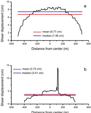
As an alternative choice to calculate a representative shear displacement of a PFC2D fracture, we suggest using the median value. By using the median value of shear displacement of the smooth joints that represent a PFC2D fracture, multiple large shear displacement values, numerical artefacts in the model, are overlooked. Moreover, in case of an isolated fracture under shear as shown in Figure 5a, choosing the median displacement instead of the mean displacement is more conservative due to the fact that for the kind of shear displacement distribution observed in the models, the median is usually larger than the mean value, as also shown in Figure 10a.

For the highest level of conservativeness of the safety assessment of the repository, one should use the maximum displacement as a representative displacement of a fracture. However, for choosing the maximum displacement, the correction scheme for “rattlers” and “virtual damage” introduced above should be applied first. In this report, we choose to use the median displacement since the correction scheme was developed after and not applied to the results presented in the following chapters. In case of an fracture as Fracture #2 in Figure 5c, choosing the median instead of the mean displacement is acceptable due to the fact that the median is not sensitive as the mean value to the large peak values in the model that come from the numerical artefact. Moreover, the difference between the mean and the median is less than 10%. Figure 10b shows the median and mean values of the shear displacement for a fracture intersected by other fractures under shear as Fracture #2.

(23)

Figure 10. Shear displacement profile of (a) an inclined isolated PFC2D fracture (Figure 5a) and (b) an intersected fracture (Fracture #2 in Figure 5c) under shear loading and mean and median values for the representative shear displacements.

2.8. The Consultants’ assessment

PFC2D can reproduce the parabolic distribution of shear displacement of an isolated fracture along its trace that match the analytical solution in Eq. (1). The parabolic distribution of shear displacement disappears when a fracture is intersected by other fractures. When fractures are intersecting, there are many jumps and drops of the shear displacement along their traces due to the intersections. This behaviour is verified by the modelling results by FRACOD2D, which is a numerical code based on different theory from PFC2D. However, as presented in the previous section, some spikes of the shear displacement plots in the PFC2D modelling cannot be explained by the behaviour of the fracture intersections. The reason for such spikes is investigated and it is found to be due to stress and displacement singularity due to the fact that particles are not allowed to break even under high stress concentrations (no “virtual damage”) and that some particles detach from the neighbouring particles (“rattler particles”). Material failure and detachment/fragmentation would probably occur in nature in the rock at such locations with complex fracture settings. This cannot be simulated with PFC2D. Such features are the key factors in generating large displacement spikes at fracture intersections, which can be regarded as a numerical artefact. Although, the Consultants suggest a possible solution that can properly eliminate the numerical artefacts, in this report the Consultants propose that the median displacement is used on the results of fracture displacements containing the spikes. The choice of the median value is expected to filter away the effect of the numerical artefacts arising at the intersections between fractures, and still provide enough conservative estimates of shear displacement, especially for the isolated fractures. -600 -400 -200 0 200 400 600 0 2 4 6 8 10 mean (6.77 mm) median (7.46 mm) Distance from center (m)

Shear dis plac ement (c m) -600 -400 -200 0 200 400 600 0 5 10 15 mean (3.73 mm) median (3.41 mm) Shear dis plac ement (mm)

a b mean (6.77 cm) median (7.46 cm) (c m ) mean (3.73 cm) median (3.41 cm)

(24)

(25)

3. The Forsmark repository model

3.1. Model generation and boundary conditions

The Forsmark repository model is constructed based on the integrated geological model by Stephens et al. (2015). The horizontal section model contains deformation zones and fracture domains at 460 m depth inside the proposed repository volume in the SKB’s Local Model Volume. The deformation zones marked in dark red shown in Figure 11a are steeply dipping or vertical and have a trace length at the surface longer than 3000 m. Zones marked in dark green are steeply dipping or vertical and have surface trace length less than 3000 m. Zones marked in light green are gently dipping.

The PFC2D horizontal section model is shown in Figure 11b and contains almost all the deformation zones in the integrated geological model by Stephens et al. (2015), except the light green gently dipping deformation zones ZFMA1, ZFMA2, ZFMB7, ZFMB8 and ZFMF1. Exclusion of these deformation zones is due firstly to the 2D nature of the PFC2D model and, secondly to the fact that the zones are cutting the repository depth far from the planned location of the deposition panels.

Fractures in the repository (“target fractures”) are embedded in the models and shown in red in Figure 11b. The repository fractures are stochastically generated in a 3D space within the SKB’s Local Model Volume, and then their traces at the depth of the repository (460 m) are determined. The traces of the fractures are extracted from the Discrete Fracture Network (DFN) realisations and embedded in the PFC2D model (see Appendix 2 in Yoon et al., 2014) after converting to a format readable in PFC2D. Black dots in the figure show the heat emitting particles in the PFC2D models that have assigned heat power equivalent to disposed spent fuel canisters. The maximum horizontal stress (black) and the minimum horizontal stress (red) are shown in Figure 11b by two sets of arrows indicating their orientation. The initial magnitude of the maximum and the minimum horizontal stresses is 40 MPa and 22 MPa, respectively. The model is compressed by controlling the velocity of the particles on the outer layer (light blue region) until the internal stresses match the nominal magnitude of the maximum and minimum horizontal stresses. After this, the movement of the particles on the outer layer is fixed throughout the modelling. The in situ stresses are total stresses and the effect of pore pressure was not taken into account.

(26)

Figure 11. (a) Integrated geological model by Stephens et al. (2015), and (b) PFC2D horizontal section model containing the deformation zones (green), the repository target fractures (red) and the heat emitting particles (black dots). ZFMWNW0809A is the deformation zones used for the earthquake modelling in this study. The arrows indicate the orientations of the maximum and the minimum horizontal stresses.

b

a

SH

Sh

(27)

Figure 12. (a) NW-SE cross-section through the candidate volume in the structural model (Figure 4-12 in SKB, 2011) showing rock domains and deformation zones, (b) vertical section of the PFC2D model containing deformation zones (green), fractures at the repository depth (red) and the particles representing deposition panels (black dots), (c) enlarged view of the repository area in (a), and (d) initial temperature field with depth.

The PFC2D model of the vertical section is generated based on the section of the integrated geological model on the NW-SE vertical plane through the candidate volume as shown in Figure 12a (SKB, 2011). The PFC2D vertical section model is shown in Figure 12b and contains the deformation zones (green), repository fractures (red) and the particles representing the deposition panels (black dots). As for the horizontal section model, the velocity of the particles on the outer layer (light blue region in Figure 12b) is controlled until the initial stress state at the depth of the repository reaches approximately 40 MPa and 12.5 MPa for the maximum

horizontal stress and for the vertical stress, respectively. The velocity of the particles on the outer layer is programmed to change in order to achieve stresses with a depth gradient of 0.078 MPa/m for the maximum horizontal stress and 0.026 MPa/m for the vertical stresses, respectively. The in situ stresses are total stresses and the effect of pore pressure was not taken into account.

After the stresses are applied, a temperature field is assigned with a depth gradient of 23°C/km, computed from the mean in situ temperatures at different depths at Forsmark (Sundberg et al., 2008). Convective heat boundary conditions are assigned to the top outer particle layer in order to simulate heat loss to the atmosphere by forced convection that maintain a temperature of 0°C at the top surface as in SKB’s

Panel A Panel B Panel C Panel D

A1 B5 N N W 0101 B4 B23 B6 A3 B1 A7 A4 A5 A6 WNW0123 B7 A2 A8 F1 866 b c a d Te m p ( oC)

(28)

modelling in Hökmark et al. (2010). As in the horizontal section model, the movement of the outer layer particles is fixed after the present-day initial stresses are applied. However, due to the forced convective heat loss condition assigned to the top layer of the model, where the particle temperature is forced to maintain 0°C by removing the heat, the thermal boundary condition leads to decrease in the size of the particles due to thermal contraction, and consequently has the effect of softening the top boundary.

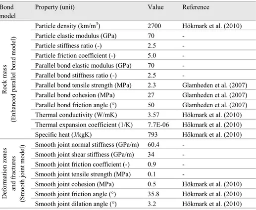
The parameters used for the Forsmark repository models in for the horizontal and vertical settings are listed in Table 1. For the rock mass, the enhanced parallel bond model (see definition by Itasca, 2012) was used, which allows to input the tensile strength, cohesion and friction angle to the particle contacts where deformations and failure potentially occur without need of heavy calibration campaigns of the bond parameters. For the deformation zones and the repository target fractures, we used the smooth joint model (Mas Ivars et al., 2011).

Table 1. Model parameters used for generation of the PFC2D Forsmark repository model.

Bond

model Property (unit) Value Reference

R ock ma ss (E nh an ced p ar al lel b on d m od el )

Particle density (km/m3₎ ₂₇₀₀ _{Hökmark et al. (2010)}

Particle elastic modulus (GPa) 70 - Particle stiffness ratio (-) 2.5 - Particle friction coefficient (-) 5.0 - Parallel bond elastic modulus (GPa) 70 - Parallel bond stiffness ratio (-) 2.5 -

Parallel bond tensile strength (MPa) 2.3 Glamheden et al. (2007) Parallel bond cohesion (MPa) 27 Glamheden et al. (2007) Parallel bond friction angle (°) 50 Glamheden et al. (2007) Thermal conductivity (W/mK) 3.57 Hökmark et al. (2010) Thermal expansion coefficient (1/K) 7.7E-06 Hökmark et al. (2010) Specific heat (J/kgK) 793 Hökmark et al. (2010)

De fo rm ati on z on es an d fra ctu re s (S m oot h joi nt m ode

l) Smooth joint normal stiffness (GPa/m) 60.4 -

Smooth joint shear stiffness (GPa/m) 34 - Smooth joint friction coefficient (-) 0.9 - Smooth joint tensile strength (MPa) 0.1 -

Smooth joint cohesion (MPa) 0.5 Hökmark et al. (2010) Smooth joint friction angle (°) 35.8 Hökmark et al. (2010) Smooth joint dilation angle (°) 3.2 Hökmark et al. (2010)

3.2. Heat loading

Due to the 2D nature of the horizontal section models, i.e. no heat dispersion in the out-of-plane direction, adjustment of the heat power output is necessary. It is confirmed by COMSOL modelling (see Appendix D) that using the full canister heat power shown in Figure 13 (black curve) assigned to the 1 m thick insulated panel plane results in extremely high temperatures. Therefore, an assumption is made that about 10% of the total heat energy coming from a full size canister (9034 GJ represented by the area under the black curve in Figure 13) and spreading in a 3D volume goes into the 1 m thick insulated panel. Lowering the curve is done by

(29)

results in a total heat energy of 1073 GJ (red curve in Figure 13) input in the model with 1 m thickness in the out-of-plane direction.

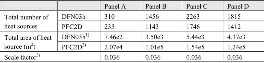
Another adjustment of the heat power curve is necessary due to the size of the particles in the PFC models. The total number of heat point sources equivalent to spent fuel canisters in the model is 5844, which is obtained by applying the Full Perimeter Intersection Criterion to the DFN03h fracture realization (Yoon et al., 2014). However, due to larger size of the particles in the PFC2D model compared to the size of the deposition holes in the repository, a scaling factor is introduced based on the particle size where the heat source is applied. Table 3 lists the scaling factors applied to the heat emitting particles in each panel of the repository. The scaling factors are applied to the modified heat power curve in Figure 13 (red curve) which is assigned to the heat emitting particles (black dots in Figure 11b).

For the PFC2D vertical section model, the original heat power curve (black curve in Figure 13) is applied to the particles that are grouped into individual panels (blue dots in Figure 12c). The following equation for the heat power is assigned to the grouped particles representing the panels, assuming line heat source similar to that of Probert and Claesson (1997):

∑ Eq. (2)

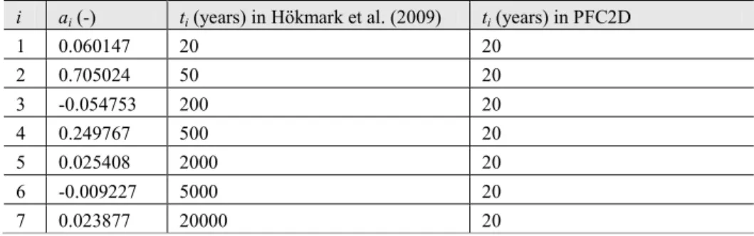
where px is the distance between deposition tunnels (40 m). Coefficients ai and ti

from Hökmark et al. (2009) are listed in Table 2.

Figures 14 and 15 show the heat power curves applied to the heat emitting particles for the simultaneous and sequential heating of the panels for the horizontal and the vertical section models, respectively. Different starting times of the curves for the cases of sequential heating are due to the fact that the time taken to complete the deposition of the canisters in each panel is taken into account. It is assumed that it takes about 3 days to place one canister in a deposition hole. Therefore, for example, the heat curve for the Panel A in the horizontal section model (black curve in Figure 14b) starts at 2.5 years, because it takes 2.54 years to place 310 canisters (310 canisters × 3 days/canister × 1 year / 365 days = 2.54 years). And the heat release from the canisters is designed to start after all 310 canisters have been placed at the deposition locations.

Table 2. Parameters used for the heat power curves in the PFC2D horizontal section model. i ai (-) ti (years) in Hökmark et al. (2009) ti (years) in PFC2D

1 0.060147 20 20 2 0.705024 50 20 3 -0.054753 200 20 4 0.249767 500 20 5 0.025408 2000 20 6 -0.009227 5000 20 7 0.023877 20000 20

(30)

Table 3. Scaling factors used for the heat power curves in the PFC2D horizontal section model.

Panel A Panel B Panel C Panel D Total number of

heat sources

DFN03h 310 1456 2263 1815 PFC2D 235 1143 1746 1412 Total area of heat

source (m2₎ DFN03h

1) _7.46e2 _3.50e3 _5.44e3 _4.37e3

PFC2D2) _2.07e4 _1.01e5 _1.54e5 _1.24e5

Scale factor3) _0.036 _0.036 _0.036 _0.036 1)_{Area of deposition hole is 2.40 m}2_.

2)_{Area of particle heat source in the PFC2D model is 86.5 m}2_.

3)_{Scale factor = total area of heat source in the repository layout with DFN03h / total area}

of heat source in the PFC2D model.

Figure 13. Power curve with modified ti parameters (red) and the original power curve of full

size canister (black) for the PFC2D modelling of the horizontal section.

1 10 100 1000 0 500 1000 1500 2000

full size canister (9034 GJ) modified curve (1073 GJ)

Powe

r (W

)

(31)

Figure 14. Power curves applied to the heat particles for (a) simultaneous heating and (b) sequential heating of the panels for the PFC2D horizontal section model.

1 10 100 1000 0 20 40 60 80 Powe r (W) Time (a) 1 10 100 1000 0 20 40 60 80 panel A particles panel B particles panel C particles panel D particles Powe r (W) Time (a)

a

b

(32)

Figure 15. Power curves applied to the heat particles for (a) simultaneous heating and (b) sequential heating of the panels in the PFC2D vertical section model.

Several particles are selected in the horizontal section model to monitor the temporal evolution of the temperature and the thermal stresses as shown in Figure 16a. Four particles, #1 to #4, are located at the centre of the panels and other four particles, #5 to #8, are located outside the panel areas. These monitoring particles (Figure 16b) are selected to compare the temperature evolution as a function of time simulated in the PFC2D model with SKB’s results from 3DEC models (Hökmark et al. 2010). However, the locations of particle #1 and #3 do not exactly match with the locations of Scanline C and Scanline A in SKB’s 3DEC model shown in Figure 16b due to unknown exact coordinates of the scanlines in SKB’s model.

1 10 100 1000 10000 0 10 20 30 40 50 Powe r (W ) Time (yrs) 1 10 100 1000 10000 0 10 20 30 40 50 Panel A particles Panel B particles Panel C particles Panel D particles Powe r (W ) Time (yrs)

a

b

(33)

Figure 16. Particles selected for monitoring the evolution of temperature and thermal stress (#1 - #4: at the panel area centres, #5 - #8: outside the panel areas) and the locations of the scanlines in SKB’s 3DEC model (Hökmark et al. 2010).

3.3. Earthquake loading

An earthquake at a specific deformation zone is simulated by releasing the stored strain energy under a given stress condition at the smooth joint contacts forming the activated deformation zone. In order to accumulate strain energy and store it along the trace of a deformation zone, the bond strength of the smooth joint contacts at the earthquake hosting deformation zone is multiplied by a factor of 1000. This allows deformation at the smooth joints contacts, but failure of the smooth joint is not allowed. Thereafter the model is compressed until the internal stresses reach the target present-day principal stresses (in Table 4, SH and Sh for the horizontal section model, and SH and Sv for the vertical section model). Here, we used the total stress and did not include 5 MPa pore fluid pressure at the depth of the repository. Deformation and failure of other smooth joints in the model are allowed during the whole calculation. Two deformation zones are selected for the earthquake modelling, one in the horizontal and one in the vertical section models. These are

ZFMWNW0809A and ZFMA3 as indicated red in Figure 17.

Table 4. Absolute stress components as the present-day initial stress fields for the PFC2D horizontal and the vertical section models.

Model Stress components (MPa) Remark and reference SH Sh Sv

Horizontal 40 22 - Most likely stress field (Martin, 2007)

Vertical 40 - 12.5 At the repository depth of 460 m, Reverse stress _{field (Fälth et al., 2010)}

-1500 -1000 -500 0 500 1000 1500 2000 -1500 -1000 -500 0 500 1000 1500 2000 Titel Y-Ac hs e Titel X-Achse 1 2 3 4 5 6 7 8 a _A b B C D

(34)

Figure 17. Deformation zones selected for the earthquake modelling (red) in the PFC2D (a) horizontal and (b) vertical section models.

The release of the accumulated strain energy in the earthquake hosting deformation zone is simulated by lowering the bond strength of the smooth joint contacts with a

multiplication factor 10-20_{for the tensile and cohesion strength of the smooth joints.}

In addition to this, friction and dilation angles of the smooth joints are lowered to 10% of their original values, i.e. from 35° to 3.5°. Such measure was taken to mimic a rupturing process and the strain energy release when the fracture asperities are lost due to the earthquake slip. Lowering of the joint normal and shear stiffness was not considered because of the minimal impact on the rupturing process. This is

suggested as further study as it is expected to have influence on the post-earthquake behaviour. Upon releasing the strain energy, a seismic wave is generated at the activated deformation zone and propagates through the model. Models are given a few seconds to respond to the seismic wave.

The seismic moment magnitudes M0/m of the simulated earthquakes correspond to

the seismic energy released at the earthquake hosting deformation zones with 1 m thickness in the out-of-plane direction. Therefore, the seismic moment refers to a 1 m thick slice of the real deformation zones. In order to take into account of the seismic energy from a full size deformation zone, it is assumed that real deformation zones have a width equal to their length, therefore the Rupture Area (RA) = length ×

width = length2_{. The ratio of 1:1 between the rupture length and the rupture width is}

-1800 -1200 -600 0 600 1200 1800 -1800 -1200 -600 0 600 1200 1800 y (m) x (m) ZFMWNW0809A

a

b

-4000 -3000 -2000 -1000 0 1000 2000 3000 4000 -2000 -1500 -1000 -500 0 ZFMA3 D C B A NW-SE (m) Dep th (m)

(35)

a conservative assumption but also reasonable as seen in Figure 18 from the rupture length vs. rupture width relation for tectonic earthquakes on natural faults from

different sources in the literature. The simulated seismic moment M0/m is then

multiplied by the length to take into account of the seismic moment resulting from

activation of the full size fault surface. The seismic moments (M0) that correspond to

the full size deformation zones are then converted to moment magnitudes (Mw) using

the equation by Hanks and Kanamori (1979):

⁄ Eq. (3)

Figure 18. Rupture length vs. rupture width relation of the natural tectonic earthquake faults (WC1994: Wells and Coppersmith, 1994); Data1 in M2005: 2D earthquake slip inversion models in Manighetti et al.,2005; Data2 in M2005: Teleseismic earthquake slip models in Manighetti et al., 2005). 0 20 40 60 80 100 0 20 40 60 80 100 6:1 3:1 1:1 WC1994 Data1 in M2005 Data2 in M2005 R up tu re w id th (k m ) Rupture length (km)

(36)

3.4. Modelling cases

Table 5 lists the modelling cases covered in this study. Descriptions of the key features of the models are provided at the bottom of the table.

Table 5. Modelling cases performed in this study.

Loading1)

Model type2) Heating3); Stress4); DFN5); DZEQ; tEQ6) Chapter

T (H) Sim Mls DFN03h 4

Seq Mls DFN03h 4

T (V) Sim Rsf DFN06v 5

Seq Rsf DFN06v 5

T+EQ (H) Sim Mls DFN03h ZFMWNW0809A 100 yrs 6 T+EQ (V) Sim Rsf DFN06v ZFMA3 100 yrs 6

1) _{Loading conditions}

 T: Thermal induced

 T+EQ: Thermal and earthquake induced

2) _{Model types}

 H: Horizontal section model (Figure 11b)  V: Vertical section model (Figure 12b)

3) _Heating

 Sim: All panels are heated simultaneously  Seq: Panels are heated in sequence, ABCD

4) _{Present-day initial stress fields}

 Mls: Most likely stress (SH vs. Sh in Table 4)  Rsf: Reverse stress field (SH vs. Sv in Table 4)

5) _{Discrete Fracture Network (DFN)}

 DFN03h: the most conservative realization for the horizontal model (Figure 11b)  DFN06v: the most conservative realization for the vertical model (Figure 12b)

(37)

4. Modelling of heat induced seismicity

and fracture shear – horizontal section

model

4.1. Temperature distribution

The distribution of rock temperature increase at several selected times resulting from simultaneous heating of the panels in the horizontal section model is shown in Figure 19. Panel A undergoes a maximum temperature increase at 50 years. The maximum temperature increase appears approximately 100 years after the start of the heating for Panels B, C and D. The temperature increase in Panel C lasts longer than in other panels as it contains the largest number of heat emitting particles (1746, see Table 3).

Figure 20 shows the temporal changes of the rock temperature increase monitored at several selected particles in the model as illustrated in Figure 16a. Particle #1 and Particle #4 show larger rates of temperature decay compared to that of Particle #2 and Particle #3. This is due to the fact that Panel A contains the smallest number of canisters and Panel D is distant from Panel C, which leads to less heat conduction from Panel C to D. Unlike the temperature increase monitored at the centre of the panel areas, Figure 20b shows a continuous increase of the rock temperature at the points at a distance of about 100 m outside the panel areas (Particle #6 and #7) until 1,000 years, after that a decrease of the rock temperature. The calculations were time consuming and it was decided to stop at 3,000 years when the curves in Figure 20 showed clear signs of temperature decrease after the peak temperature.

(38)

Figure 19. Distribution of the rock temperature increase at several selected times resulting from simultaneous heating of all panels in the PFC2D horizontal section model.

∆T (degC)

50 yrs 100 yrs

200 yrs 500 yrs

(39)

Figure 20. Temporal changes of the rock temperature increase monitored at several selected particles (Figure 16a, Particles #1 to #4: at the centre of panel areas, Particles #5 to #8: outside the panel areas) resulting from simultaneous heating of all panels in the PFC2D horizontal section model.

Distribution of rock temperature increase at several selected times from sequential heating of the panels is shown in Figure 21. Figure 22 shows the temporal changes of the rock temperature increase monitored at several selected particles in the PFC2D horizontal section model. The temperature increase in Panel A is the highest at 50 years. However, the peak of the temperature increase at the centre of Panels B, C and D appear approximately 100 years after start of the heating. Same as in the simultaneous heating, the model was run up to 3,000 years and Figure 22b shows that the temperature increases at the particles outside the panel areas (Particles #6 and #7) hit the peak temperature at 1,000 years and then decreases.

1 10 100 1000 0 10 20 30 40 50 Particle 1 Particle 2 Particle 3 Particle 4 Temp er ature inc reas e ( o C) Time (yrs) 1 10 100 1000 0 10 20 30 40 50 Particle 5 Particle 6 Particle 7 Particle 8 Temp er ature inc reas e ( o C) Time (yrs) a b

(40)

Figure 21. Distribution of the rock temperature increase at several selected times resulting from sequential heating of the panels in the PFC2D horizontal section model.

∆T (degC)

50 yrs 100 yrs

200 yrs 500 yrs

(41)

Figure 22. Temporal changes of rock temperature increase monitored at several selected points (Figure 15a, Particles #1 to #4: at the centre of panel areas, Particles #5 to #8: outside the panel areas) resulting from sequential heating of panels in the PFC2D horizontal section model.

4.2. Thermally induced stresses

Thermally induced stresses are monitored at the selected particles (Figure 16a). Figure 23 shows temporal changes of the stresses resulting from simultaneous

heating in the direction of the major (σ1) and minor (σ2) initial principal stresses.

The maximum change in σ1 is about 60 MPa and takes place at the centre of Panel D

(Figure 23a, Particle 4). The maximum change in σ2 at the panel centre is about

40 MPa and occurs in Panel B (Figure 23c, Particle 2). The largest change in σ1

outside the panels takes place at Particle #7 and is about 45 MPa, which is between

Panel C and D (Figure 23b). The changes in the σ2 outside the panels are below

20 MPa (Figure 23d).

The temporal evolution of the thermal stresses from the sequential heating (Figure 23) is similar to that resulting from the simultaneous heating and reach a peak between 50 and 200 years for the particles at the centre of the panels.

1 10 100 1000 0 10 20 30 40 50 Particle 1 Particle 2 Particle 3 Particle 4 Temp er ature inc reas e ( o C) Time (yrs) 1 10 100 1000 0 10 20 30 40 50 Particle 5 Particle 6 Particle 7 Particle 8 Temp er ature inc reas e ( o C) Time (yrs) a b

(42)

Figure 23. Temporal evolution of thermally induced major principal stress (σ1) (a) at the panel centres (Particles #1 to #4), (b) outside the panels (Particles #5 to #8), and minor principal stresses (σ2) (c) at the panel centres (Particles #1 to #4), (d) outside the panels (Particles #5 to #8), resulting from simultaneous heating of all panels in the PFC2D horizontal section model.

1 10 100 1000 0 10 20 30 40 50 60 70 Particle 1 Particle 2 Particle 3 Particle 4 Ther mal stres s, 1 (MP a) Time (yrs) 1 10 100 1000 0 10 20 30 40 50 60 70 Particle 5 Particle 6 Particle 7 Particle 8 Ther mal stres s, 1 (MP a) Time (yrs) 1 10 100 1000 0 10 20 30 40 50 60 70 Particle 1 Particle 2 Particle 3 Particle 4 Ther mal stres s, 2 (MP a) Time (yrs) 1 10 100 1000 0 10 20 30 40 50 60 70 Particle 5 Particle 6 Particle 7 Particle 8 Ther mal stres s, 2 (MP a) Time (yrs) a c b d

(43)

Figure 24. Temporal evolution of thermally induced major principal stress (σ1) (a) at the panel centres (Particles #1 to #4), (b) outside the panels (Particles #5 to #8), and minor principal stresses (σ2) (c) at the panel centres (Particles #1 to #4), (d) outside the panels (Particles #5 to #8), resulting from sequential heating of the panels in the PFC2D horizontal section model.

4.3. Induced seismicity

The heat emitted from the canisters results in thermally induced stress changes as shown in Figures 23 and 24 and consequently causes slip of the pre-existing fractures and failure of the rock mass. Figure 25 shows the distribution of thermally induced seismic events accumulated over (a) 100 years and (b) at 1,000 years after start of simultaneous heating of the repository panels. Figure 26 shows the results for the sequential heating.

1 10 100 1000 0 10 20 30 40 50 60 70 Particle 1 Particle 2 Particle 3 Particle 4 Ther mal stres s, 1 (MP a) Time (yrs) 1 10 100 1000 0 10 20 30 40 50 60 70 Particle 5 Particle 6 Particle 7 Particle 8 Ther mal stres s, 1 (MP a) Time (yrs) 1 10 100 1000 0 10 20 30 40 50 60 70 Particle 1 Particle 2 Particle 3 Particle 4 Ther mal stres s, 2 (MP a) Time (yrs) 1 10 100 1000 0 10 20 30 40 50 60 70 Particle 5 Particle 6 Particle 7 Particle 8 Ther mal stres s, 2 (MP a) Time (yrs) a b c d

(44)

Figures 25 and 26 contain information on the induced seismic event magnitudes.

Seismic moment M0/m due to the slip of the smooth joint is calculated using the

following equation:

Eq. (4)

where G is the shear modulus (30 GPa), A is the smooth joint area (m2_{, smooth joint}

length ×1 m thickness in the out-of-plane direction), and d is the shear displacement

(m). The moment magnitude Mw is then computed using Eq. (3).

The distributions of the seismic events that accumulated over 100 year after the start of heating (Figure 25a for the simultaneous and Figure 26a for the sequential

heating) demonstrate that the magnitudes of the seismicity is mostly below Mw1.1

and distributed within the footprint of the panels. However, the distribution of the seismic events evolves with time and tends to cluster at the area of high fracture density and at the areas where the fractures are intersecting one another and with the deformation zones.

Seismicity clusters tend to migrate away from the panel areas over time as shown in Figure 25b and Figure 26b for the simultaneous and sequential heating, respectively.

The magnitudes observed at 1,000 year are mostly below Mw2.2 for the

simultaneous and sequential heating.

The results should be interpreted with caution, because some of the large

displacements of the smooth joints at the intersections can be numerical artefacts as discussed in Section 2.6. If the stress concentrated at the intersections is high enough to induce failure of the rock mass in the neighbouring areas, this can lead not a single large seismic event but to multiple events distributed over an area with magnitudes lower than the single large event could have.

(45)

Figure 25. Distribution of the thermally induced seismic events accumulated over (a) 100 years and (b) 1,000 years after start of the simultaneous heating of all the panels in the PFC2D horizontal section model with DFN03h realization.

a

Mw Mw

b

-1800 -1200 -600 0 600 1200 1800 -1800 -1200 -600 0 600 1200 1800 y (m ) x (m) -0.1 0.4 0.6 0.9 1.1 -1800 -1200 -600 0 600 1200 1800 -1800 -1200 -600 0 600 1200 1800 y (m ) x (m) 1.0 1.5 1.7 2.0 2.2