98:28 Study of the Possibility of Localising a Channel Instability in Forsmark-1

Study of the Possibility of Localising a

Channel Instability in Forsmark-1

J. K-H. Karlsson and I. Pázsit

Department of Reactor Physics Chalmers University of Technology

Undersökning av möjligheten att lokalisera

en kanalinstabilitet i Forsmark-1

J. K-H. Karlsson och I. Pázsit

Chalmers Tekniska Högskola, Avd. för Reaktorfysik 412 96 Göteborg

Sammanfattning

Vid uppstart av Forsmark-1, efter revision 1996, uppträdde en speciell typ av insta-bilitet. Instabiliteten yttrade sig genom svängningar i neutronflödestätheten (LPRM-signa-lerna). Svängningarna hade störst amplitud i en liten region nära kanten av härden och minskade i amplitud med ökande avstånd. Detta beteende skiljer sig från andra typer av instabilitet som har uppträtt tidigare i kokvattenreaktorer. De andra typerna är de globala (ifas i hela härden) och regionala (motfas mellan två härdhalvor) svängningarna. En detalje-rad analys visade att orsaken troligen var en s.k. kanalinstabilitet (density wave oscillation), vilken är en rent termohydraulisk instabilitet. Vid revisionen 1997 kontrollerades ett trettio-tal patroner i det misstänkta området och en patron befanns då vara osätad. En osätad patron orsakar en förändring i enfastryckfallet för kanalen, vilket kan leda till en kanalinstabilitet.

Syftet med föreliggande undersökning är att rapportera om utveckling och tillämp-ning av en metod för att underdrift lokalisera positionen för störtillämp-ningen (den termohydrau-liska oscillationen), vilken sannolikt överensstämmer med positionen för den felaktiga patronen (störningskällan). Metoden består av två delar. Den första delen består i att visua-lisera svängningarna i neutronflödestätheten för att få en kvalitativ uppfattning om situatio-nen. Den visuella undersökningen ger information om vilken typ av svängning det rör sig om, typen av störningskälla och en grov uppfattning om dess position. Den visuella under-sökningen har dessutom potential för att kunna göras on-line och användas för stabilitets-övervakning av reaktoroperatören. Den andra delen av metoden består av en kvantitativ (algoritmisk) metod för att lokalisera störningskällan. Metoden bygger på en reaktorfysika-lisk modell både av störningskällan och av överföringsfunktionen mellan källan och de resulterande svängningarna i neutronflödestätheten. Modellen anpassas till mätdata från LPRM-signalerna, vilket ger störningskällans position. Metodens styrka ligger i dess rums-upplösning som i princip ligger på patronnivå, d.v.s. den är bättre än avståndet mellan två närliggande LPRM sonder. Algoritmen har testats med simulerade data, samt tillämpats på Forsmarks mätningar av störningen. I fallet med Forsmarks kanalinstabilitet fann metoden störningskällans position i närheten av den patron, vilken vid revisionen visade sig vara osä-tad. Syftet med studien var i huvudsak att utveckla och testa metoden. För tillämpning av metoden på ett mer effektivt sätt och med högre noggrannhet, så krävs ytterligare utveck-ling av framförallt realistiska överföringsfunktioner.

Study of the Possibility of Localising a

Channel Instability in Forsmark-1

J. K-H. Karlsson and I. Pázsit

Chalmers University of Technology, Dept. of Reactor Physics 412 96 Göteborg

Summary

A special type of instability occurred in the Swedish BWR Forsmark 1 in 1996. In contrast to the better known global or regional (out-of-phase) instabilities, the decay ratio appeared to be very high in one half of the core and quite low in the other half. A more detailed analysis showed that the most likely reason for the observed behaviour is a local perturbation of thermohydraulic character, e.g. a density wave oscillation (DWO), induced by the incorrect positioning of a fuel assembly (an “unseated” assembly). In such a case it is of large importance to determine the position of the unseated assembly already during operation such that it can be easily found during reloading.

The subject of this paper is to report on development and application of a method by which the position of such a local perturbation can be determined. The method can be separated into two parts that support and complement each other. First a visualisation technique was elaborated which displays the space-time behaviour of the neutron flux oscillations in the core (i.e. a movie of the LPRM signals). This visualisation expedites a very good qualitative comprehension of the situation and can be useful for the operators. It also gives an important basis for the application of the localisation algorithm. Second, a quantitative (algorithmic) localisation method, suited for this type of perturbation and based on reactor physical models of the perturbation and of the transfer function between the perturbation and the flux oscillations, was elaborated. This latter takes noise spectra from selected detectors as input and yields the perturbation position as output. The strength of the method lies in its potentially high spatial resolution, which is smaller than the typical distance between two adjacent LPRM detectors. The method was tested on simulated data, and then applied to the Forsmark measurements. The location of the disturbance, found by the algorithm, is in accordance with independent judgements for the case, and close to a position where an unseated assembly was found during refuelling. The purpose of this study was to develop and test the localisation method. To apply the method more effectively and with a high level of accuracy, it needs some further development in particular of the transfer function.

1. INTRODUCTION

The local instability event which is analysed in this report has been described in several reports previously (Refs. [1] and [2]). Hence it will not be described in detail here. It was discovered as a half-core instability phenomenon, and a large part of its analysis con-cerns the instability properties such as the decay ratio. However, the position of the instabil-ity is also of interest, because an inspection of the fuel assembly or assemblies in which the instability occurred may reveal the reason of its appearance. One hypothesis is that the instability arose due to an improper “seating” of the assembly. Without having a qualified guess about the approximate position of the instability, it is practically not possible to find a reason because there is no possibility to check every fuel assembly due to time constraints.

Attempts have been made also before this study in order to locate the instability position. One possibility is to make an intuitive guess based on the distribution of signal amplitudes. The only algorithmic method used so far was the noise contribution ratio or sig-nal transmission path asig-nalysis methods (Refs. [2] and [3]). In these methods a multivariate analysis of several LPRM signals is used and one of them is pointed out as the driving force for the other detector signals. The position of the perturbation is then assumed to lie either at the position of the LPRM or in its neighbourhood.

There exist however another method by which the location of the perturbation can be determined. One can utilize the fact that any localised perturbation induces a space-dependent neutron noise. The noise amplitude and phase decay with increasing distance from the source, thus the space dependence carries information on the position of the source. By modelling the noise source in some functional form, and calculating the reactor physical dynamic transfer function of the core, the induced neutron noise can be expressed via formulas, either analytical or numerical, in which the position of the perturbation is included as an argument. By the use of such relationships or formulas, a method of localisa-tion can be elaborated, by which the posilocalisa-tion of the perturbalocalisa-tion can be found from the measured neutron noise and the calculated transfer function of the system. Such a strategy was used in the past for the localisation of an excessively vibrating control rod in a VVER-type pressurized water reactor (Refs. [4] and [5]).

The advantage of such a method is that it uses reactor physics knowledge on the spatial attenuation of the neutron noise from a source. Due to this fact, the spatial resolution of the localisation procedure is high; it can in principle point out any position in the core, and not only the discrete detector positions. In practice, of course, the accuracy of the method can be low for various reasons that will be discussed later on. The important point at this stage is that there is no principal limitation involved in the spatial resolution of the method.

Even within the methodology outlined above, there are two different strategies that can be applied for the actual localisation procedure. As described shortly, one of them can be called a general method and the other a (source-) specific method. Both were originally planned to be tested in the present study. In the general method, nothing is assumed in advance about the type (space dependence) of the noise source. In this method, the com-plete space-dependence of the noise source in the core is reconstructed. The spatial structure

of the reconstructed noise source will reveal if the noise source (perturbation) was evenly distributed or localised, and in the latter case, where (in which core position(s)). This strat-egy can only be applied if a large number of detector signals at different points is available. In the specific method, a concrete assumption is made on the functional form of the pertur-bation. In other words, this method requires some independent information on the perturba-tion. Assuming that the perturbation is localised at one (unknown) point is an example for such an assumption. If such an information is available, and a correct noise source model is used, this method can be very effective with a relatively limited number of detectors. This is why in practice, hitherto only this latter method was used (in the case of locating a vibrating absorber mentioned above), while the general method was only tested in conceptual studies so far (Ref. [6]).

It turned out in the beginning of the study that the number of detectors available in the Forsmark measurements was not sufficient to make the general method applicable. In addition, the few tests performed even with this limited number of detectors made it clear that application of this method leads to prohibitively long computer running times, due to the involved calculations that need to be performed. Thus, in this study the general method was dropped and only the specific method was elaborated, tested and applied.

This work will be described and developed in more detail in a future journal publi-cation. Further, the methods developed in the course of this investigation have been col-lected in a number of computer codes, which have been written as scripts for use with MATLAB. These scripts are at the free disposal of the Swedish Nuclear Power Inspector-ate. Other interested parties can obtain these scripts from the Dept. of Reactor Physics, Chalmers University of Technology.

2. INVESTIGATION OF THE NOISE SOURCE

Basically, there are two different types of localised perturbations. One of them is the so-called “reactor oscillator” (Ref. [7]) which is conceptually equal to a localised absorber of variable strength. This perturbation has been investigated extensively in the past, but not with the purpose of localisation. The second type is represented by the lateral vibrations of an absorber rod. This noise source has been also the matter of thorough inter-est in the past. However, because of its practical relevance, also the possibility of localising a vibrating control rod from the induced neutron noise has been investigated and applied (Ref. [4]). It has to be added immediately that the spatial structure of the neutron noise induced by a vibrating absorber and an absorber of variable strength is rather different. This is manifested in the fact that the corresponding noise expressions, on which the localisation procedure is based, are also quite different. Hence, the localisation procedure, elaborated and used for the vibrating rod problem, cannot be applied to the localisation of a channel type instability; rather, a new algorithm need to be elaborated. This was made and will be reported in this study.

Intuitively, it is expected that a channel instability is equivalent to a reactor oscilla-tor, i.e. an absorber of variable strength. However, before this assumption is actually used, one must assure that this is indeed the case. This is only possible by an investigation of the spatial structure of the noise, i.e. the LPRM detector signals. One way of doing this is to

consider the spatial distribution of the oscillation amplitudes and the phase relationships between the detectors and around the oscillation frequency. In this study however a more effective and informative way was introduced and used for this purpose. This method uses a visual inspection of the joint space-time behaviour of the noise in the core directly in the time domain. An animation or motion picture of the space- and time-dependent neutron noise was constructed. In Fig. 1, one cycle of the instability oscillation is shown in sequence from this movie.

An analysis of a few minutes of the display yields the following conclusions on the perturbation:

• the spatial peaks in the noise field are all generated by an absorber of variable strength rather than by a perturbation corresponding to lateral vibrations. (This latter could be the case for instance if two adjacent channels oscillated in opposite phase);

• there is one primary spatial peak (i.e. localised perturbation) and one secondary peak of smaller amplitude than the primary. Further, there are also perturbations at other posi-tions that appear and vanish in a non-stationary way;

• the oscillations are not stationary in time, not even for the two principal peaks. However, for these latter, one may assume approximate stationarity such that spectral analysis methods can be applied;

• the individual localised perturbations are quite well separated in space.

Based on the above, it was assumed that the perturbation consists of a single oscil-lation of the variable strength absorber type. The spatial separation between any two pertur-bations appearing concurrently was large enough (larger than the attenuation length of the noise, see later) such that two different perturbations that occur simultaneously can be local-ised separately, by using a suitably selected set of detectors.

3. THE LOCALISATION METHOD

3.1 The noise source model and the localisation algorithm

As is usual with noise calculations, it is convenient to express the noise in the fre-quency domain as a convolution of the transfer function (Green’s function) of the unper-turbed system, and the noise source (Ref. [8]):

(1)

Here, is the transfer function, discussed later, and is the noise source,

or perturbation, that induces the noise. It consists of the fluctuations of the macroscopic cross sections which appear in the time-dependent diffusion equations.

A noise source of variable strength at a fixed position can be represented

func-tionally as (2) δφ(r,ω) =

∫

2 3 4 5 6 7 1 2 3 4 5 6 7 y Time = 220.64 s x 2 3 4 5 6 7 1 2 3 4 5 6 7 y Time = 220.88 s x 2 3 4 5 6 7 1 2 3 4 5 6 7 y Time = 221.12 s x 2 3 4 5 6 7 1 2 3 4 5 6 7 y Time = 221.36 s x 1 2 3 4 5 6 7 1 2 3 4 5 6 7 −5 0 5 y Time = 221.84 s x 1 2 3 4 5 6 7 1 2 3 4 5 6 7 −5 0 5 y Time = 221.6 s x 1 2 3 4 5 6 7 1 2 3 4 5 6 7 −5 0 5 y Time = 222.08 s x 1 2 3 4 5 6 7 1 2 3 4 5 6 7 −5 0 5 y Time = 222.32 s x

Fig. 1. The figure shows the amplitude of the flux in the x-y plane for a single cycle. a) b) c) d) e) f) g) h)

In reality, the noise source is not a -function, rather it has a finite volume. This fact how-ever can be accounted for, as will be discussed later on. Applying (2) in (1), the noise, as

measured by a detector at position , is given as

(3)

In this expression, is known from measurement, and can be

calcu-lated as a function of its arguments. However, and are noise source properties, and

they are not known in a practical case. Since the main interest lies in the determination of

the source position (localisation), we will use the notation as the argument for the position

of the source in the algorithm. Thus, we have succeeded in the localisation procedure when

we obtain .

To this order we consider an expression for the ratio of two detector signals, which will be given as

(4)

In this expression, the source strength is eliminated. The l.h.s. is known from

meas-urement, and the unknown perturbation position can in principle be obtained as the value

(more precisely, one of the values) which, when substituted into (4), satisfies the equation. Using only one pair of detectors, in general there will be a whole line on the 2-D plane, in

which the search for is made, each point of which satisfies (4). Such a line was called a

“localisation curve” in Ref. [4]. One needs at least one more detector to obtain one or two more localisation curves, such that the intersection of such lines gives the true perturbation position. This is a kind of triangulation, and was used in the localisation of a vibrating con-trol rod.

In the present work we have however elaborated a new method which is more powerful than the one based on the localisation curves. The method can moreover utilize very effectively the fact that in the present case we have access to more than the theoretical minimum requirement of three detectors, and that thus there is a certain redundancy in the measurement. It is also more algorithmic than the method of using the localisation curves because it avoids the subjective step of finding a multiple intersection point of many curves and yields the perturbation position as an explicit result.

The method is formulated as follows. Having access to detectors, one can select

pairs and corresponding ratios of the type (4). Then, for the pair and , one

defines the quantity

(5)

Clearly, theoretically is zero in an ideal case if . This would be the case if no

background noise, no measurement error existed etc. In practice however all these exist,

thus in general (5) will deviate from zero for all values. It can however be expected that

δ r_i δφ(r_i,ω) = γ ω( )G r( _i, ,r_p ω) δφ(r_i,ω) G r( _i, ,r_p ω) γ ω( ) r_p r r = r_p δφ(r_i,ω) δφ(r_j,ω) --- G r( i, ,r ω) G r( _j, ,r ω) ---= γ ω( ) r r n n n( –1)⁄2 r_i r_j δ_ij( )r δφ(ri,ω) δφ(r_j,ω) --- G r( i, ,r ω) G r( _j, ,r ω) ---– ≡ δ_ij( )r r = r_p r

the deviation from zero will be minimum for the true rod position. Thus, we define the opti-mization function as

(6)

Then, the source position can be derived as

(7) In practice, the above needs to be developed a little further. Namely, it is not the Fourier-transformed detector signals that are used, rather their auto- and cross-spectra. Thus the above needs to be re-formulated in terms of spectral quantities. This is straightforward, and the following relationships can be used to construct a function whose minimum yields the position of the perturbation:

(8)

(9)

where, in general, is complex. The optimization function in this case becomes

(10)

The position of the perturbation is then given as before by

(11) The localisation method, as described above, can be extended to localize several concurrent noise sources. However, the complexity of the method increases somewhat and the amount of computational effort needed increases significantly. However, as long as the noise sources are not over-lapping each other substantially, the multiple source method does not necessarily improve the localisation but it does still increase the complexity. Because of the above reasons, we have only applied and tested the single source method.

3.2 Calculation of the transfer function

In this study only simple reactor models were considered, in which the transfer function can be calculated analytically. In particular, we have used one-group diffusion the-ory, one group of delayed neutrons and a bare, homogeneous cylindrical reactor in

2-dimen-sional geometry. This model is essentially the same as the one used in the study and

application of the method of localising a vibrating control rod (Ref. [4]).

f r( ) δ_ij2( )r i j,

∑

∑

∑

As described in the earlier reports Refs. [8] and [6], the transfer function can be obtained from the following equation:

(12) where

(13)

and is the zero reactor transfer function. In earlier works, for diagnostic purposes,

(12) was solved by using the so-called power reactor approximation, which means assum-ing

(14)

This is equivalent with the assumption of lying at the plateau frequency region

where

, (15)

and also assuming $ (which holds to a good approximation in power reactors). In

this approximation, the transfer function can be given in the compact form

(16)

This transfer function was one of the two used and tested in this study. The other transfer function used is obtained by solving (12) without approximation. This is given as (Ref. [8])

(17)

This transfer function is much more realistic and advanced than the one given by (16). It is complex, and therefore it describes also phase delay effects. The advantage of the simpler form (16) is that it is computationally much simpler, which may be a significant advantage since the transfer function has to be evaluated a very large number of times during the local-isation procedure. By comparing CPU times for a locallocal-isation procedure using the above two transfer functions, some extrapolation to the expected CPU times when using even more complicated (heterogeneous) transfer functions can be made.

With the model developed in this section, in particular with a point-like source, the

noise will be proportional to the Green’s function. This latter diverges at , as is seen

G ∆ (r r, ,_p ω)+B2( )ω G r r( , ,_p ω) = δ(r–r_p) B2( )ω B₀2 1 1 ρ_∞G₀( )ω ---–     = G₀( )ω B2( )ω = 0 ω λ ω β Λ« « ⁄ G₀( )ω 1 β ---≈ ρ_∞ = 1 G r( , , ,α r_p α_p) 1 2π --- R 2 r2r2_p⁄R2–2rr_pcos(α α– _p) + r2+r2_p–2rr_pcos(α α– _p) ---      ln = G r r( , ,_p ω) 1 4 --- Y[ ₀(B r–r_p)– = 2–δ_{n 0,} ( )Y_n(BR)J_n(Br_p) J_n(BR) ---J_n( )Br cos(n(α α– _p)) n=0 ∞

∑

from (16) and (17). This is not a serious problem during the localisation procedure as long

as only a discrete set of values is used in the minimisation procedure such that never

coincides with any of the . This is what was also done in the

present study.

In reality the divergence does not exist since the noise source is not a -function,

but has a finite volume, i.e. is distributed over a certain area. In the case of channel instabil-ity it is more realistic to assume a noise source that is constant over the area of a fuel assem-bly in which the instability occurs. In that case, instead of (3), the neutron noise will be given as

(18)

Here, the transfer function is the same as before, whereas the integration is carried out over

the area of the assembly which contains now as its centre. It is easy to confirm that (18)

does not diverge for any values of .

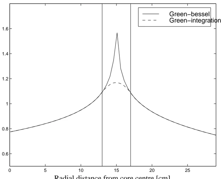
Although the divergence problem can be avoided even with point-like sources, it is important to investigate the spatial behaviour of the noise given by (18) as compared to that given by (3). This is because the underlying principle of the localisation is the space dependence of the neutron noise. If (18) would predict a significantly different space

dependence as a function of than (3), then the former should be used in the

algo-rithm instead. This question was investigated numerically, and it was found that except the very vicinity of the noise source, the neutron noise by (3) and (18) has a nearly identical dependence on the distance from the source (Fig. 2).

The conclusion is that as long as the closest detector in a measurement lies outside the fuel channel where the instability (perturbation point) is present, the simpler formula (3) can be used in the localisation. This is always fulfilled in a BWR, since the detectors are sit-uated in between the fuel channels. This is a very large advantage since again, the noise for-mulas need to be evaluated a very large number of times and application of (18) instead of (3) would increase the CPU time of the localisation with several orders of magnitude.

4. TEST OF THE ALGORITHM WITH SIMULATED DATA

To get some hands-on experience with the algorithm, and to get some estimate of its performance, it was first tested in simulation tests. These tests were conceptually similar to those performed in the study of the algorithm for the localisation of a vibrating control

rod. The starting point is the selection of the position of the source, , and a few detector

positions . To simplify the simulations, we have selected the minimum

possible number of detectors, which is three. Then the induced noise at these detector posi-tions is calculated by (3), after which the calculated noise values were used in the localisa-tion algorithm (5) and (7). The minimisalocalisa-tion procedure was performed in the whole 2-D plane, yielding an absolute minimum. Since the perturbation position is known in advance in these tests, the correctness of the result, and thus the performance of the algorithm, can

r r r_i, i = 1 2 3...n, , δ δφ(r_i,ω) γ ω( ) G r( _i, ,r′ ω)dr′ F

∫

be judged. The significance of the test is motivated among others also by the fact that the expressions in (7) and (11), respectively, may have several minima, and there is no prior proof of the hypothesis that the perturbation position yields the absolute minimum. Espe-cially in the case of “disturbed” or “not clean” detector signals, such a proof may not exist at all since the deviations between the assumption of the model and reality are not known in exact quantitative terms. Thus the only way of finding the answers to such questions is to perform numerical simulations with both “clean” and “contaminated” signals (the contami-nation is also simulated). Another goal of the test is to check the sensitivity of the algorithm to disturbing effects such as background noise, statistical measurement error etc. Even if the existence of these does not lead to the occurrence of a global minimum at a position com-pletely different from that of the true perturbation position, it will lead to deteriorated accu-racy of the method. The simulation of the perturbed signals is achieved by adding a random number of a few percent to each calculated detector signal before performing the localisa-tion step (7).

Tests were made by using both transfer functions of Section 3.2, expressions (16) and (17), mainly to see difference between the two regarding computational effort, i.e. required CPU time. Regarding performance, we only report on the results with the more advanced transfer function (17). A layout of the selected source position and detector posi-tions is seen in Fig. 3. The absolute value and phase of the induced neutron noise are shown in Fig. 4 over the whole cross-section of the core, i.e. not only in the three detector positions (which are indicated in Fig. 3) that will be used in the localisation algorithm. It is seen how the amplitude of the noise decreases and the phase delay increases with increasing distance

0 5 10 15 20 25 0.6 0.8 1 1.2 1.4 1.6 Green−bessel Green−integration

Fig. 2. A comparison of the results obtained close to the perturbation

position if a -function model of the source is used (solid line) or a source

with a finite volume (dashed line).

δ

from the source. From the quantitative results an attenuation length, i.e. a distance within which most of the noise amplitude change takes place, can be extracted. This attenuation length is about half of the radius of the core. The space-dependence also agrees qualitatively with the one seen in Fig. 1. The magnitude of the attenuation length is also in agreement with the fact that the oscillations are felt in about one half of the core.

Expression (7) whose absolute minimum is to give the source position, is shown in Fig. 5. It is seen that it has a relatively simple structure, with only one minimum which is very well discernible, and it also coincides with the source position. This is reassuring,

although the smoothness of the function depends partly on the use of a homogeneous

23 46 69 92 115 30 210 60 240 90 270 120 300 150 330 180 0

Fig. 3. The localised source position is marked by ‘X’. The detectors

used in the localisation are indicated by ‘●’ and the actual source posi-tion by ‘O’. In Fig. 3b the localisaposi-tion algorithm was disturbed by the addition of extraneous random noise to the detector signals.

a) 23 46 69 92 115 30 210 60 240 90 270 120 300 150 330 180 0 b) X X f r( )

−100 −50 0 50 100 −100 −50 0 50 100 0 0.1 0.2 0.3 0.4 0.5 x Calculated noise y Magnitude (abs) −100 −50 0 50 100 −100 −50 0 50 100 −5 −4 −3 −2 −1 0 x Calculated noise y Phase [degrees]

Fig. 4. The spatial distribution of the calculated noise amplitude and its phase

Calculated noise amplitude

reactor model. In an inhomogeneous reactor model it may not be as simple; this question will be investigated in the future.

The results of the algorithm for one case are shown in a different way in Fig. 3a, where a direct estimation on the precision can be visually made. The figure shows the results of the algorithm both for the case when pure (unperturbed) signals were used in the localisation step, and the case when perturbed signals were used (Fig. 3b). In the latter case a random number with a variance of 5% of the mean value of each signal was added to all three detector signals. It is seen that in the latter case the precision of the algorithm deterio-rates, as expected. For perturbations of this magnitude, the deterioration is not large.

5. APPLICATION OF THE METHOD TO FORSMARK DATA

In the measurements, power spectra are used rather than frequency transformed raw signals. Accordingly, in this analysis, the form (8)-(11) of the localisation algorithm was used. The layout of the core, with all detectors available in the measurement, is shown in Fig. 6. The number of detectors is much larger than the required minimum of 3 detectors, which was used in the simulation tests. Actually, it was not practical to use all detectors at a time in a localisation run, only a limited set. There are two reasons why a limited set of detectors is more efficient than using all of them. First, as both the measurement “movie” (Fig. 1) and the simulated results (Fig. 4) show, the amplitude of the noise diminishes rela-tively fast away from the source, with a relaxation length smaller than the core radius. Since the background noise (i.e. noise from sources other than the instability) can be expected to

−100 −50 0 50 100 −100 −50 0 50 100 −2 −1 0 1 x Minimization surface (real part, log10−scale)

y

be a smooth function of core position, e.g. follow the space dependence of the static flux, the relative weight of the useful noise is low in the signal of detectors that are far away from the source. Thus, the localisation is more accurate if only detectors from the same half or quadrant of the core are used where the source position is situated. The second reason for why using detectors around the suspected source position is effective is that the present algorithm is based on the assumption of one single source being active at a time. The meas-urement movie, on the other hand, makes it likely that at least one or two noise sources are acting, even if not stationarily, only in a sporadic manner. Fortunately, these potential sources are all separated from each other by a distance comparable with or larger than the noise attenuation length. By selecting groups of detectors around each potential source, the effect of other sources is minimised and the various source positions can be determined sep-arately by applying the single-source algorithm individually. It is this strategy that has been used in the present work.

Selecting a group of detectors is of course a somewhat subjective moment. Since the result of the localisation depends on the detectors used in the localisation algorithm, the selection of a set of detectors introduces an element of arbitrariness into the procedure. This kind of influencing the outcome of the results is justified by the fact that the conditions in a practical case do not exactly correspond to the idealised conditions assumed in the algo-rithm. The selection of a “most suitable” set of detectors is made in order to minimize the consequences of this deviation between practice and theory, and is performed by using reac-tor physics expertise.

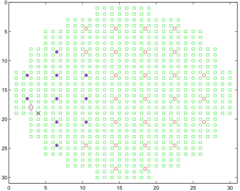
We have tried to locate two noise sources, primarily the principal one close to LPRM 10, and a secondary one close to LPRM 7. Again, in the localisation both transfer functions were used, but results will be shown here with the complex transfer function only. The results of the first case, concerning the primary source, are shown in Fig. 6. The figure also shows the detectors that were selected in this localisation procedure. The result of the localisation is also shown in Fig. 7, where it is seen that the identified position is neighbour-ing to a position (18,3) where an unseated fuel assembly was found after revision 1997.

Varying the number and position of the detectors used in the procedure will natu-rally affect the result of localisation. This was also investigated by choosing various detec-tor sets. As long as detecdetec-tors are taken mostly from the west half of the core, the variation of the result is quite moderate. Choosing detectors from the other half of the core will lead to significantly different results. This is in accordance with the previous reasoning on the selection of the most suitable set of detectors above. At any rate, the result shown in Figs. 6 and 7 is the one that appears to be most plausible.

Results of the localisation of the secondary source, including the position of the detectors used is shown in Fig. 8. This position too corresponds quite well to the local oscil-lations seen in the movie. Hence it is also demonstrated that the two noise sources could be identified separately by the use of suitably selected detector sets, and by applying the single source localisation algorithm.

51.7975 103.595 155.3925 207.19 30 210 60 240 90 270 120 300 150 330 180 0

Fig. 6. The position of the source (X) as obtained by the

localisa-tion method using the detectors (●).

X 51.7975 103.595 155.3925 207.19 30 210 60 240 90 270 120 300 150 330 180 0

Fig. 8. The position of the secondary source as obtained by the

indicated detectors (●) in the localisation method.

6. CONCLUSIONS AND FUTURE WORK

The main purpose of this study was to test the applicability of the localisation tech-nique in a practical case, using the Forsmark measurements. Such an algorithm has not been used and tested before. The study, both in simulations and with measured data, showed that the algorithm works satisfactorily. It was demonstrated that the resolution of the method is higher than the distance between the detectors in the core. It was also seen that two or three sources can be localised individually if they are separated sufficiently well in space, with applying the single source localisation algorithm by using suitable selected sets of detectors. One weakness of the method in its present form is the very simple core model used in the calculation of the transfer function. Besides of using one-group theory, the most important restriction is the use of a homogeneous bare reactor model. Core inhomogenei-ties, reflector, and most important, control rod patterns cannot be taken into account in the present model. The most important task in the further development of the method is to extend it to two energy groups, include a reflector, and take into account the inhomogene-ous core structure. This will require fully numeric methods, and perhaps parallel computing techniques due to the large complexity of the calculational task.

0 5 10 15 20 25 30 0 5 10 15 20 25 30

Fig. 7. The position of the source as obtained by the localisation method and

the position of the unseated fuel element is indicated by a cross and a diamond character, respectively.

ACKNOWLEDGEMENTS

The authors are greatly indebted to Pär Lansåker and Thomas Smed, who invited us to study the problem of localisation of a channel instability. They also supported this work with the transfer of measurement data, information on the core state and valuable sug-gestions for improving the analysis.

This work was financially supported by a grant from the Swedish Nuclear Power Inspectorate (SKI), Grant No. 14.5 971559-97233.

REFERENCES

[1] Lansåker P. (1997), Forsmark internal report FT-Rapport 97/485 (In Swedish) [2] Oguma R. (1997), Swedish Nuclear Power Inspectorate (SKI) Report 97:42 [3] Söderlund M. (1997), Forsmark internal report FT-Rapport 97/295 (In Swedish) [4] Pázsit I. and Glöckler O. (1984), Nucl. Sci. Engng. Vol. 88, pp. 77-87

[5] Pázsit I. and Glöckler O. (1988), Nucl. Sci. Engng. Vol. 99, pp. 313-328 [6] Glöckler O. and Pázsit I. (1987), Ann. nucl. Energy Vol. 14, pp. 63-75

[7] Bell G. I. and Glasstone S. (1970), Nuclear Reactor Theory, Van Nostrand Reinhold Company, New York

[8] Pázsit I and Garis N. S. (1995), Swedish Nuclear Power Inspectorate (SKI) Report 95:14 (In Swedish)