02:28 Evaluation of the SCANAIR Computer Code

Research

Evaluation of the SCANAIR Computer Code

Lars Olof Jernkvist

Ali Massih

November 2001

ISSN 1104–1374 ISRN SKI-R-02/28-SE

The overall goals for SKI rearch are: • to give a basis for SKI:s supervision

• to maintain and develop the competence and research capacity within areas which are important to reactor safety

• to contribute directly to the Swedish safety work.

This project has mainly contributed to the strategic goal of giving a basis for SKI:s supervision by means of an independent evaluation of the computer code SCANAIR with respect to its applicability for licensing purposes. The project has also contributed to the goal of maintaining and developing the competence and research capacity within Sweden.

SCANAIR was developed by IRSN and was obtained through SKI:s participation in the OECD/NEA CABRI Water Loop Project.

The results from the limited study of SCANAIR has mainly been positive, the report especially emphasizes the unique pellet material model. The report however indicates that some of the models used should be improved; clad material model and heat transfer models clad – water. The conclusion is that SCANAIR is an adequate computer code for predicting thermal-mechanical behavior of a fuel rod during a postulated RIA although the code would benefit from further calibration to experimental data.

Project information:

Project manager: Ingrid Töcksberg, Department of Reactor Technology, SKI Project number: 14.6-010185/01088

Research

Evaluation of the SCANAIR Computer Code

Lars Olof Jernkvist

Ali Massih

Quantum Technologies AB

Uppsala Science Park

SE-751 83 Uppsala

Sweden

November 2001

SKI Project Number 01088

This report concerns a study which has been conducted for the Swedish Nuclear Power Inspectorate (SKI). The conclusions and viewpoints presented in the report are those of the author/authors and do not necessarily coincide with those of the SKI.

List of contents

2.1.1 Fuel, clad and shroud thermal conductance ... 4

2.1.2 Pellet-clad gap ... 4 2.1.3 Coolant channel ... 5 2.1.4 Numerical method ... 5 2.2 Structural analysis ... 6 2.2.1 Governing equations... 6 2.2.2 Deformation phenomena ... 8 2.2.3 Numerical method ... 12

2.3 Fission gas behavior ... 13

2.3.1 Intra-granular gas bubbles ... 13

2.3.2 Inter-granular gas bubbles ... 14

2.3.3 Flow of gas through pores ... 15

2.3.4 Numerical method ... 16

3 SCANAIR interface: input and output data... 19

3.1 Input data to SCANAIR ... 19

3.2 Output data from SCANAIR ... 21

4 Code implementation and documentation ... 23

4.1 Code implementation... 23

4.2 Code documentation ... 24

5 Computations... 25

5.1 REP4 test case ... 25

5.2 Comparison of SCANAIR with STRUCTUS ... 30

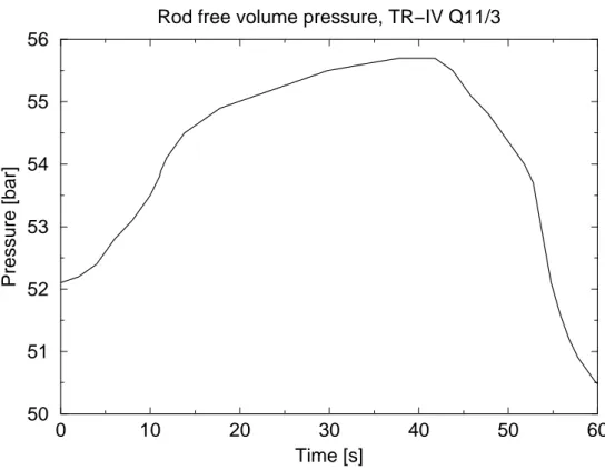
5.3 TRANS-RAMP IV test case... 34

5.4 REP Na-2 test case ... 40

6 Concluding remarks... 43

Appendix A: REP4 test case... 47 Appendix B: TRANSRAMP-IV test case ... 55

Summary

The SCANAIR computer code, version 3.2, has been evaluated from the standpoint of its capability to analyze, simulate and predict nuclear fuel behavior during severe power transients. SCANAIR calculates the thermal and mechanical behavior of a pressurized water reactor (PWR) fuel rod during a postulated reactivity initiated accident (RIA), and our evaluation indicates that SCANAIR is a state of the art computational tool for this purpose.

Our evaluation starts by reviewing the basic theoretical models in SCANAIR, namely the governing equations for heat transfer, the mechanical response of fuel and clad, and the fission gas release behavior. The numerical methods used to solve the governing equations are briefly reviewed, and the range of applicability of the models and their limitations are discussed and illustrated with examples.

Next, the main features of the SCANAIR user interface are delineated. The code requires an extensive amount of input data, in order to define burnup-dependent initial conditions to the simulated RIA. These data must be provided in a special format by a thermal-mechanical fuel rod analysis code. The user also has to supply the transient power history under RIA as input, which requires a code for neutronics calculation.

The programming structure and documentation of the code are also addressed in our evaluation. SCANAIR is programmed in 77, and makes use of several general Fortran-77 libraries for handling input/output, data storage and graphical presentation of computed results. The documentation of SCANAIR and its helping libraries is generally of good quality. A drawback with SCANAIR in its present form, is that the code and its pre- and post-processors are tied to computers running the Unix or Linux operating systems.

As part of our evaluation, we have performed a large number of computations with SCANAIR, some of which are documented in this report. The computations presented here include a hypothetical RIA in a high-burnup fuel rod. This test case is used to check the validity of SCANAIR installation in a new computer environment, but also to examine the output response of the code to an RIA-type load. Moreover, we have used independent computational methods to verify and compare some of the SCANAIR results for this reference case. The outcome is encouraging.

In addition, we have attempted to simulate with SCANAIR a ramp test performed at the Studsvik R2 reactor, and a rod in the Studsvik TRANSRAMP-IV project was selected for this purpose. Although SCANAIR is not designed to simulate “moderate” transients like the one considered here, we have found the results on fission gas release and clad plastic strain in fair agreement with measured data.

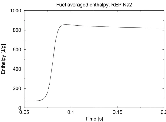
Finally, we have performed computations on an existent RIA test made on a pre-irradiated rod in the CABRI reactor, to wit the REP-Na2 rod in the REP-Na test series. Rod Na2 was subjected to a fast RIA-type pulse with a pulse-width of 0.9 ms and a peak linear power density of about 40 MW/m. Also for this test case, SCANAIR exhibited good performance with reasonable execution times on personal computers with the Linux operating system.

We have not subjected SCANAIR to extensive testing and benchmarking against experimental data, nor to a wide-range of parametric studies to locate possible faults of the code in analyses of highly irradiated fuel rods under RIA. However, our evaluation and testing indicate that the models used for pellet and clad (visco)plastic deformation and axial mixing of released fission products should be improved. Nevertheless, our limited study with SCANAIR has been positive. Although it would benefit from further calibration to experimental data, we believe that SCANAIR is an adequate computer code for predicting thermal-mechanical behavior of a fuel rod during a postulated RIA.

Sammanfattning

Datorprogrammet SCANAIR, version 3.2, har utvärderats med utgångspunkt från programmets förmåga att analysera, simulera och prediktera beteendet hos kärnbränsle under kraftiga effekttransienter. SCANAIR beräknar det termiska och mekaniska beteendet hos en kärn-bränslestav i en tryckvattenreaktor (PWR) under en postulerad reaktivitetstransient (RIA), och vår utvärdering visar att SCANAIR är ett framstående beräkningsverktyg för detta ändamål. Vår utvärdering börjar med en genomgång av de grundläggande teoretiska modellerna i SCANAIR, nämligen de styrande ekvationerna för värmetransport, mekaniskt beteende hos bränslekuts och kapsling, samt frigörelse av gasformiga fissionsprodukter. De numeriska metoder som används för att lösa dessa ekvationer berörs, och modellernas tillämplighet och begränsningar diskuteras och belyses med exempel.

De viktigaste dragen hos SCANAIRS användargränssnitt beskrives härnäst. Programmet behöver en stor mängd indata, som används för att definiera det utbränningsberoende begynnelsetillståndet till den simulerade reaktivitetstransienten. Dessa indata måste överföras i ett speciellt format från ett beräkningsprogram för termomekanisk bränslestavanalys. Användaren måste dessutom föreskriva effekthistorien under RIA, vilket förutsätter ett program för reaktorfysikberäkningar.

Även programkodens struktur och dokumentation belyses i vår utvärdering. SCANAIR är programmerat i Fortran-77, och använder ett flertal generella bibliotek skrivna i detta språk för att hantera in/utdata, datalagring och grafisk presentation av resultat. Dokumentationen av SCANAIR och dess bibliotek är i stort av god kvalitet. En nackdel är att SCANAIR och dess pre- och post-processorer i nuvarande form är bundna till datorer med operativsystemet Unix eller Linux.

Ett stort antal beräkningar med SCANAIR har utförts som en del av vår utvärdering, och resultat från några av dessa beräkningar presenteras i rapporten. Till dessa hör en beräkning av en hypotetisk RIA i en högutbränd bränslestav. Detta testfall används för att verifiera installeringen av SCANAIR i en ny datormiljö, men även för att studera programmets respons med avseende på ett RIA-liknande belastningsfall. Vi har dessutom använt oberoende beräkningsmetoder för att verifiera SCANAIRS beräkningsresultat för detta referensfall. Resultaten är positiva.

Vi har även försökt använda SCANAIR för att simulera ett ramptest utfört i R2-rektorn i Studsvik, och en bränslestav från Studsvikprojektet TRANSRAMP-IV valdes för denna simulering. Trots att SCANAIR egentligen ej är avsett för simulering av ”milda” transienter som denna, så har vi funnit att beräknad fissionsgasfrigörelse och plastisk kapslingstöjning stämmer relativt väl med mätdata.

Slutligen har vi genomfört beräkningar av ett befintligt RIA-prov, vilket utförts på en bestrålad bränslestav i CABRI-reaktorn, nämligen stav REP-Na2 i provserien REP-Na. Denna stav utsattes för en RIA-liknande effektpuls med en pulsvidd om 0.9 ms och en maximal längdvärmebelastning om 40 MW/m. SCANAIR fungerade väl även för detta fall, och gav rimliga exekveringstider på Linuxbaserade persondatorer.

Vi har i detta arbete ej genomfört någon omfattande provning eller verifiering av SCANAIR, ej heller någon heltäckande parameterstudie för att lokalisera eventuella svagheter vid analyser av högutbrända bränslestavar under RIA. Vår utvärdering och provning visar dock att modellerna för kutsens och kapslingens (visko)plastiska deformation samt modellen för axiell blandning av frigjorda fissionsprodukter bör förbättras. Detta oaktat, så har vår begränsade utvärdering av SCANAIR givit positiva resultat. Även om programmet skulle gagnas av ytterligare kalibrering gentemot experimentella data, så anser vi att SCANAIR är ett fullgott beräkningsprogram för att prediktera bränslestavens termomekaniska beteende under postulerade reaktivitetstransienter.

1 Introduction

The purpose of this report is to document an evaluation made of the computer program SCANAIR. The SCANAIR code is designed to simulate the thermal-mechanical behavior of a pressurized water reactor (PWR) fuel rod during a reactivity insertion accident (RIA). A reactivity insertion accident in fission-reactors is characterized by a rapid reactivity increase in the nuclear fuel, caused by breakdown of the reactor control system, which in turn leads to a fast power excursion up to extremely high power levels. In light water reactors (LWRs), the peak power level during RIA will be governed by the reactivity of the ejected control rod (rod worth), the Doppler coefficient, fuel power peaking factor and fraction of delayed neutrons.

The SCANAIR code is developed by the Institut de Protection et de Sûreté Nucléaire (IPSN) in collaboration with Electricité de France (EDF) within the frames of the CABRI-REP-Na program. SCANAIR consists of three basic modules, responsible for calculation of thermal dynamics, structural mechanics and fission gas behavior. The code is one-dimensional in makeup, i.e. it solves all fundamental equations for heat transfer, deformations and fission gas release with respect to the fuel rod radial direction, but takes into account each axial segment of the rod separately.

The computational flow between the three modules in SCANAIR is schematically illustrated in figure 1. The computations involve the following exchange of data between the three modules:

Thermal Dynamics Fission Gas Behavior Structural Mechanics Tem pera ture Gap gas com posi tion T em pe ra tu re G ap w idt h

Fuel hydrostatic stress

Gas pressure and fuel gaseous swelling

Thermal Dynamics ! Structural Mechanics: •

Fuel and clad temperatures are transferred from the Thermal Dynamics module to the Structural Mechanics module for calculation of thermal expansion and

temperature dependent mechanical properties of the material. • Thermal Dynamics ! Fission Gas Behavior:

Temperature data are transferred to the Fission Gas Behavior module for calcu-lation of gas diffusion coefficients, gas bubble swelling, etc.

• Structural Mechanics ! Thermal Dynamics:

The pellet-clad gap width data are transferred from the Structural Mechanics to the Thermal Dynamics module.

• Structural Mechanics ! Fission Gas Behavior

The fuel hydrostatic stress is needed in calculations of fuel fission gas swelling. • Fission Gas Behavior ! Structural Mechanics:

Fuel gaseous swelling and rod internal pressure data are transferred from the Fission Gas Behavior to the Structural Mechanics module.

• Fission Gas Behavior ! Thermal Dynamics:

Fission gas release reduces the gap thermal conductance, thus increasing fuel temperature. Gas composition data are therefore transferred to the Thermal Dynamics module.

It should be noted, that the SCANAIR code does not include a neutronic module for generating the loads (power excursion) imparted to the fuel during an RIA. Neither does it comprise steady-state models for calculation of the fuel behavior prior to the accident. These data must therefore be supplied by other external codes, and need to be inputted to SCANAIR in special formats.

According to Federici et al. (2000a), the SCANAIR code has been benchmarked against measured data obtained from the CABRI test reactor program, Papin et al. (1996) and Frizonnet et al. (1997), as well as data from NSRR, Fuketa et al. (1997). Individual models in SCANAIR have also been compared and verified with several separate effect studies, Lemoine and Balourdet (1997). For example, clad mechanical properties have been verified within the PROMETRA program, Balourdet et al. (1999). The clad-to-coolant heat transfer calculations during fast power excursions have been verified within the PATRICIA program and the transient fission gas release within the RIA-SILENE program. Moreover, the numerics of the code have been validated either against analytical solutions or against a more detailed finite element code, CASTEM, Constantinescu et al. (1998)

The organization of this report is as follows: In chapter 2, we briefly review the SCANAIR models, namely the basic equations used and assumptions made in thermal analysis, structural analysis and fission gas behavior. Chapter 3 presents an overview of the SCANAIR interface, i.e., the input and output of the code. In chapter 4, we provide some remarks on the programming aspects of SCANAIR. The results of our computations with SCANAIR are finally presented in chapter 5. In that chapter, we present the computations made on a test case used for verification of the installation and compilation of the code in our system. This case is a hypothetical RIA-like transient, postulated to occur on a high burnup PWR fuel rod. This test case has also been analyzed by use of the STRUCTUS code, for the purpose of independent model verification. In addition, the SCANAIR code has been used to simulate a ramp test made on a PWR rod (TRANSRAMP-IV) at Studsvik, and a realistic RIA simulation test performed in the CABRI test reactor. The outcome of these computations is also presented in chapter 5.

2 SCANAIR models

The SCANAIR code is designed to simulate fuel thermal-mechanical behavior during a postulated RIA. As in many steady-state fuel behavior codes, the modeling comprises three main components, Lemare and Latché (1995):

1. Thermal analysis for calculation of fuel and clad temperatures, including calcu-lation of heat transfer across the pellet-clad gap and from the clad to the coolant. 2. Structural analysis for computation of deformations and stresses.

3. Calculation of fuel fission gas release.

All the SCANAIR models are designed to treat the conditions that prevail during an RIA, i.e. applications to other reactor transients are unwarranted.

2.1 Thermal analysis

In the thermal analysis, the fuel rod and coolant channel geometry where heat transfer takes place is schematically shown in figure 2. Heat transfer takes place in the fuel, the clad tube, the fuel pellet-clad gap, the coolant and the shroud (in case of experiment simulations). Only radial heat transfer is modeled. In SCANAIR, three types of heat transfer are considered: i) heat conduction through solids, i.e. in fuel, clad and shroud, ii) gas gap conductance, iii) heat transfer into and along the coolant channel.

fuel clad coolant channel shroud

conduction

conduction + radiative heat transfer + solid-solid contact conductance

convection conduction

2.1.1 Fuel, clad and shroud thermal conductance

In the fuel, clad and shroud, the time-dependent heat transfer equation is considered in integral form:

(

∫

)

∫

∫

the heat flux. Cylindrical symmetry is assumed and the heat flux φ, which is considered only in the radial direction, is expressed as

    ∂ ∂ − = = r T er λ φ φ φv v . (2.2)

Here, is the radial unit vector, λ is the thermal conductivity of the solid, T is the temperature, and ∂/∂r denotes the partial derivative with respect to the radial coordinate. er

v

The thermal boundary condition imposed on the fuel system is that the heat flux is zero at the center of the fuel, i.e. φ =0 at r=0. At the boundaries (fuel-to-gap, gap-to-clad and so on) the Newton’s law of cooling is assumed, which is expressed as

) (T T₀ H − =

φ . (2.3)

That is, the heat flux out from the surface is proportional to the temperature difference between the surface and the surrounding medium. Here, T is the surface temperature, T0

is the bulk temperature of the surrounding medium and H is a parameter called the surface conductance or the surface heat transfer coefficient.

2.1.2 Pellet-clad gap

Heat transfer across the pellet-clad gap is achieved through 1. Conduction heat transfer through the interstitial gas, 2. Convection heat transfer through the interstitial gas,

3. Solid-to-solid conduction heat transfer through pellet-clad contact points,

4. Solid-to-solid radiation heat transfer between non-contacting parts of the surface.

Hence, the radial heat flux across the gap from pellet to clad is expressed by

(

)

gap T T

H −

=

φ , (2.4)

where Tpellet and Tclad are the pellet outer surface and clad inside surface temperatures,

respectively, and the gap heat transfer coefficient is given by

r s cv cd gap H H H H H = + + + . (2.5)

Here, are the heat transfer coefficients for conduction and convection, respectively, H

cv cd H

H ,

s is the solid-to-solid (pellet-clad) contact heat transfer coefficient, and

The term Hs depends mainly on the contact pressure and the hardness of the clad tube

material. In SCANAIR, the term is neglected, i.e. heat transfer due to free convection in the gas gap is not taken into account.

cv

H

Comment:

The governing equation used and solved for gas conduction is a steady-state heat transfer equation. Moreover, the gas mixing is considered to be instantaneous. Accordingly, the released fission gas during the transient is assumed to mix instantaneously with the gas residing in fuel rod plena. This approximation is questionable, since there is a considerable delay time for complete mixing of released gases in the fuel rod free volume, Haste (1988). Hence, the assumption of instantaneous mixing yields a higher value of the calculated gap heat flux, than if the fission products were only partially mixed. The authors of SCANAIR have recognized this weakness, and the current model is considered for improvement, Federici et al. (2000b).

2.1.3 Coolant channel

The coolant channel thermal-hydraulic model is a one-dimensional enthalpy raise model. The governing equations for thermal-hydraulic calculations are thus the conservation of mass and the conservation of energy in the axial (z) flow direction. These equations are formulated in integral form. Conservation of momentum is not considered, and the coolant pressure is therefore modeled as uniform along the rod. In the coolant channel model, the coolant is considered to be a homogenous single-phase fluid. However, boiling heat transfer in forced convection water flow (PWR conditions) and in stagnant water (NSRR1 conditions) can be modeled. The choice between the conditions is done automatically according to the coolant flow rate.

The thermal-hydraulic models for PWR conditions comprise correlations for forced convection, nucleate boiling, critical heat flux, minimum stable film temperature, transition boiling and film boiling. The models applied for NSRR conditions include correlations for natural convection, nucleate boiling, critical flux, transition boiling and film boiling. Sodium is also modeled as a possible coolant liquid in SCANAIR, primarily for simulation of CABRI-REP-Na experiments or for fast breeder reactors.

2.1.4 Numerical method

For the fuel rod, the radial heat conduction equation in integral form is discretized in space by use of the finite volume method. The mesh consists of cylindrical rings, and thermodynamic quantities are calculated in the middle of each ring or at each node, i.e. at the boundaries of the rings. In the time domain, the time discretization is made by an implicit method to ensure “unconditional” stability of the solutions.

For the coolant channel, the abovementioned conservation equations, as in the solution of the radial heat conduction equation, are discretized in finite volumes. The primary unknowns are the coolant temperatures and the exit mass flow rates at each axial segment. A Newton-Raphson method is employed to solve the set of discretized algebraic equations for temperatures of the fuel rod and the coolant channel.

1

2.2 Structural analysis

The main objective of the structural mechanics module of SCANAIR is to calculate fuel and clad deformations. A basic assumption is that the fuel rod geometry is axi-symmetric, i.e., the fuel column and the clad tube have the same symmetry axis.

The radial and axial displacements are denoted by u and w, respectively. These displacements are assumed to satisfy the following conditions:

0 = ∂ ∂ z u (2.6) and 0 = ∂ ∂ r w . (2.7) The above conditions, which imply that shear strains can be neglected, are vindicated

only if the fuel column and clad tube are sufficiently long; typically, the ratio of the cylinder length to the cylinder radius should be greater than or equal to two, i.e. l/r ≥ 2. Hence, in cylindrical coordinates, based on the preceding assumptions, the strains are reduced to three components, and can be written in the form of a column matrix:

                ∂ ∂ ∂ ∂ =           = z w r u r u z r ε ε ε θ ε , (2.8)

where εr, εθ and εz are the strain components in the radial, hoop, and axial direction,

respectively.

2.2.1 Governing equations

The equilibrium relations in radial and axial directions are expressed in axisymmetric cylindrical coordinates. The radial equilibrium equation for stresses is expressed as:

0 = − + ∂ ∂ r r r r σ σθ σ , (2.9) whereσrandσ_θ are the radial and the hoop components of the normal stress,

respectively. The boundary conditions imposed on this equation are that σ_r =−P_f , where Pf is the coolant fluid pressure, at the clad outer surface. At the clad inner surface

and at the pellet surface, σ_r =−P_i, where Pi is the rod internal pressure. However, this

boundary condition is only applied for an open pellet-clad gap, i.e. in absence of pellet-clad mechanical interaction (PCMI). In case of PCMI, fuel and pellet-clad is considered as a single solid cylinder, consisting of fuel and clad, and no boundary condition is applied on this interface.

Comment:

We note that equation (2.9) is a steady-state equation, meaning that inertia effects (acceleration of matter) are not taken into account. The general time-dependent equation of motion for material deformation, corresponding to equation (2.9) is:

r r t u σr σr σθ ρ + − ∂ ∂ = ∂ ∂ 2 2 , (2.10)

where ρ is the material density and ∂2u ∂t2 is the acceleration in the radial direction. In SCANAIR, this term is ignored without any justification.

The axial equilibrium equation is obtained by writing the equilibrium condition for matter inside a global control volume, depicted in figure 3. Two situations are foreseen: 1. No PCMI:

The axial forces acting on the volume are due solely to the coolant fluid and rod internal pressures, figure 3a. In case of fuel pellets without a central hole, we have the relations:

for the fuel pellet, (2.11)

i fo R z rdr R P fo 2 0 2π π σ =−

∫

for the clad tube. (2.12) ) ( 2 _ci2 _{i co}2 _f R z rdr R P R P co ci − =

∫

Here, σzis the axial stress, is the fuel outer radius, is the clad outer radius, is

the clad inner radius, and P

fo

R Rco Rci

f is the coolant pressure.

P_f

P_i

clad fuel

2. PCMI:

In SCANAIR, axial forces due to PCMI may either be neglected (perfect pellet-clad slip), or considered by a simple model. In the latter case, fuel and clad are assumed to be perfectly stuck, i.e. no relative axial motion between fuel and clad is allowed in those axial segments where the fuel and clad are in contact; confer figure 3b. In this case, the equilibrium conditions in equations (2.11-2.12) are applied only on the domain above the contacting segments.

P_f

P_i

clad fuel

Figure 3b: Axial force balance in case of PCMI.

In addition to the axial force balance, an axial boundary condition is applied at the bottom end of the fuel rod, where there are no fuel and clad axial displacements, i.e. w=0 at z = 0.

2.2.2 Deformation phenomena

The SCANAIR code accounts for thermo-elastic-plastic deformation of fuel and clad. For the fuel, the code also considers contributions from fission product gaseous swelling and cracking. Below is a brief description of these models.

2.2.2.1 Fuel deformation

The total fuel strain is assumed to be the sum of thermal expansion, elastic strain, plastic strain, fission product gaseous swelling and deformation due to fuel cracking, so called pellet relocation.

Thermal expansion:

The method for calculation of thermal expansion in SCANAIR is not described. However, the material coefficient of thermal expansion is given for both solid and liquid phases of the fuel and is correlated to the fuel stoichiometry (the ratio of the concentration of oxygen atoms to that of the uranium atoms).

Comment:

For a non-uniformly heated cylinder of radius R with an axially symmetric temperature distribution, the radial displacement of the cylinder surface is approximately given by (Landau and Lifshitz, 1970)

∫

where α is the coefficient of thermal expansion and ν is Poisson’s ratio. If we let the cylinder be the fuel pellet column, we may estimate the surface velocity of the fuel during a step-like power pulse by taking the time derivative of usurf in eq. (2.13) and

relate it to the applied power and heat capacity of the fuel. If a volumetric heat source, q(r), is applied at time t=0, the radial temperature distribution is approximately given by

) ( ) ( ) , ( t H r q t t r T C_p = ∂ ∂ ρ , (2.14)

where Cp is the fuel heat capacity and H(t) is the Heaviside step function. In eq. (2.14),

heat conduction in the fuel is neglected, and the approximation is therefore valid only for t << 1. Combining the time derivative of eq. (2.13) with eq. (2.14), we get

∫

Equation (2.15) implies that the fuel surface velocity depends linearly on the magnitude of the power pulse q(r). Meaning that, the greater is the RIA pulse, the larger is the pellet surface velocity.

Gaseous swelling:

Fuel expansion due to the expansion of gaseous fission products in the fuel can give considerable contributions to the fuel deformation, especially for highly irradiated fuel, during an RIA. SCANAIR accounts for the variation of fuel volume due to fission product gases residing in intergranular and intragranular gas bubbles and also in the fuel original pores. The volume occupied by bubbles depends strongly on the hydrostatic stress, σ_{h (}σ_r σ_θ σ_z)/3 in the fuel material. At equilibrium, the gas bubble pressure depends on the surface tension term and the hydrostatic stress through

+ + =

h

R

P= 2γ −σ , where γ is the surface tension of the solid and R is the bubble radius. Fuel swelling (the relative increase in volume ∆V V) due to fission gases in porosity is calculated by an equation of state in the form

      + =       ∆ h p pore kT b c V V σ ρ . (2.16)

Here, ρ is the fuel density, cp the number of gas atom in pores per unit of fuel mass, b is

the van der Waal gas coefficient for xenon, k the Boltzmann constant, and T is the absolute temperature.

Elastic deformation:

The elastic deformation of the fuel is calculated using Hooke’s generalized law in an isotropic form that relates the principal stresses to principal elastic strains through Young’s modulus and Poisson’s ratio. These parameters are correlated to temperature and porosity of the material.

Fuel cracking:

Cracking of the fuel due to a sharp temperature gradient and non-uniform thermal expansion during power variations contributes to fuel displacements. In SCANAIR, cracks are supposed to occur in planes normal to the principal stresses σθandσz. Only

radial and axial cracks are thus modeled, and circumferential cracks are not considered. A cracked region in the fuel is assumed not to resist tensile stresses. The strain due to cracking is thereby defined as the additional inelastic strain that must be introduced to relax a possible tensile stress to zero.

Comment:

SCANAIR does not generate cracks during the power transient. It assumes that either the fuel is already cracked, whereupon no tensile stresses can exist, or it is uncracked and assumed to have an elasto-plastic behavior. To this end, it should be noticed that the fuel gaseous swelling can be strongly affected by what assumption is made about the cracks, Latché et al. (1995). If the fuel is assumed cracked, σθandσzare always zero or

negative, and the hydrostatic stress σh in eq. (2.16) will have a different value than if the

fuel were assumed as uncracked.

Fuel plasticity:

SCANAIR only considers instantaneous fuel plasticity, whereas deformation due to creep or viscoplastic deformation is neglected. Plastic strains are calculated using the Prantl-Reuss flow rule, which relates the plastic strain increment to the stress derivative of the yield function; see section 2.2.3. Plastic deformation takes place when the von Mises equivalent stress equals the flow stress, σ0, of the material. The flow stress of

UO2 is supposed to be a function of temperature only, i.e., no strain hardening is

considered. In SCANAIR, the flow stress of UO2 for temperatures below T=1730°C is

given by (Lamare and Latché, 1995)

460 4 . 133 0 = +T σ [MPa], (2.17)

whereas it is assumed to be zero for temperatures above 1730°C.

Comment:

Relation (2.17) for flow stress is quite unrealistic for temperatures below 1300°C. For example, the compressive flow stress of UO2 at room temperature is 960 MPa,

(Glasstone and Sesonske, 1981), which is well above the predicted value of the correlation used in SCANAIR. Actually, for T <≈ 1300°C, un-irradiated UO2 is a brittle

material, with no capacity for time-independent plastic deformation. Under tensile stress, it obeys Hooke’s law of elasticity until a critical stress value, at which the material is torn apart by brittle fracture.

This stress is called the fracture stress, see e.g. chapter 11 in Olander (1976). The fuel cracking model in SCANAIR in part considers the brittle fracture, but as mentioned above, this model treats only “pre-cracked” fuel and is not able to model generation of new cracks under the transient.

At temperatures well above 1300°C, creep is a significant deformation mechanism in UO2 fuel. Creep is not considered in SCANAIR, but the authors of the code state that

the effect of fuel creep can be studied by letting the softening temperature in the flow rule (1730°C) be a tuning parameter, Lamare and Latché, (1995). Decreasing the softening temperature is thereby equivalent to increasing the effects of creep.

Moreover, the SCANAIR formulation assumes that there is no volume change during plastic deformation of the fuel. Strictly speaking, UO2 is a porous solid and it undergoes

a volume change during plastic deformation. For this reason, the plastic behavior of UO2 is not particularly well described by the von Mises yield criterion and the

Prandtl-Reuss flow rule.

2.2.2.2 Clad deformation

It is assumed that the total clad strain is the sum of strains from thermal expansion, elastic- and plastic deformation. The clad materials considered are Zircaloy, Zr-1%Nb and stainless steel.

Thermal expansion:

Thermal expansion for the clad is calculated using a correlation between the clad volumetric expansion and temperature. The correlation used for Zircaloy is the one documented in the MATPRO handbook (1979), and it caters for both α− and β− phases of the Zircaloy material.

Comment:

Although the correlation for Zircaloy thermal expansion is taken from MATPRO, the correlation is not applied in its original form; SCANAIR treats the thermal expansion in

α-phase Zircaloy as isotropic, which is a simplification. Moreover, SCANAIR lacks true modeling of the α-to-β phase transition kinetics; the phase transition is assumed to be instantaneous.

Elasto-plastic deformation:

For elasto-plastic deformations, the Zircaloy clad is assumed to be an isotropic material with no texture. For elastic deformation, an isotropic form of Hooke’s law is used, with a simple correlation between Young’s modulus and temperature. The clad plasticity model in SCANAIR is the isotropic von Mises plasticity with an isotropic strain-hardening rule, Pontoizeau (1998). The flow stress correlation for Zircaloy is only a function of temperature, and is derived from testing of irradiated stress relief anneal Zircaloy-4, commonly used as PWR fuel clad materials.

Comment:

The models used for clad plastic deformation in SCANAIR are isotropic and independent. While the assumption of isotropy is acceptable, the assumption of time-independence is somewhat questionable, since visco-plastic effects are pronounced in Zircaloy materials, e.g. Delobelle et al. (1996).

2.2.3 Numerical method

The fuel rod is divided into a number of axial segments. Each axial segment is treated separately, i.e. the mechanical equilibrium equations and material/geometrical non-linear relations are solved axial segment by axial segment. The non-non-linear phenomena in the system consist of evolution of plastic flow and changes in the configuration of the fuel, i.e. the closure and opening of fuel pellet cracks, the gap, and/or the pellet central hole. The core of the structural mechanics module is a solver, which computes the mechanical behavior (displacements, strains and stresses) of an axial segment for a given configuration with a set of inelastic strains. Changes in configuration and evo-lution of plastic strains are treated by iteration. Figure 4 is an overview of this solver. The equilibrium equations in the radial direction of the fuel and the clad are discretized by a finite element method. The primary unknowns are the incremental displacements of each node during the considered time step. The increment of plastic strain for fuel and clad under the time step is calculated from the following two conditions:      ∂ ∂ = = σ ε eq p o eq d d ω σ σ σ , (2.18)

where dεpis the plastic strain increment, σeqis the von Mises effective stress, σ0 is the

material flow stress, and dω is a scalar to be determined. This problem is solved by a relaxation method (also called the return method), meaning that the solutions of the equilibrium equations provide von Mises effective stress levels, which in some mesh points may be larger than the flow stress. In this situation, an increment of plastic strain is postulated, such that it shall return the value of σ_eq to σ₀.

For a given configuration, find plastic strains

Change of configuration?

Configuration and plastic strains converged?

No Yes

No

Yes

2.3 Fission gas behavior

The fission gas module in SCANAIR includes models for behavior of fission product gases in the fuel and in the free volume of the fuel rod, i.e. the gap, plena, and the pellet central hole, if any. The ceramic fuel UO2, where the fission products are generated, has

a granular structure. Each grain is surrounded by other grains or by (as-fabricated) cavities, called pores. Some of these pores may be open, i.e. they are connected to the free volume. In that case, they function as conduits, through which gas can flow to fuel surfaces.

The fission process generates fission product gases as atoms in the fuel crystal structure. The SCANAIR models do not account for gas atoms in the fuel, i.e. all the fission product gases are assumed to be collected into inter- and intra-granular bubbles. Hence, the diffusive migration of gas atoms in the fuel is not modeled. Nor is the migration of granular bubbles to the pores. However, the transport of intra-granular bubbles into the grain boundaries and hence the formation of inter-intra-granular bubbles, is modeled. Also the release of inter-granular bubble gas into the pores, through which it can be conveyed to the free volume, is catered for. Figure 5 is a cartoon of the fuel microstructure, as envisioned in the SCANAIR fission gas module. In this section, we highlight some of the basic equations used in SCANAIR for modeling the aforementioned phenomena, and then close the section with some concluding remarks.

Figure 5: Fuel grains containing inter- and intra-granular gas bubbles and pores, schematically drawn. The grain size of UO2 fuel is around 12 µm.

2.3.1 Intra-granular gas bubbles

Three phenomena are modeled for describing the intra-granular gas bubbles. These are: The migration of gas bubbles through the grain due to the presence of temperature gradients, and the trapping of gas bubbles in grain boundaries.

• •

• Bubble coalescence during migration. Growth of gas bubbles caused by rapid diffusion of lattice vacancies into the gas bubbles, due to hydrostatic pressure exerted by the bubble to its solid surrounding.

The kinetic relation used for the migration of intra-granular gas bubbles to the grain boundaries is given by:

ig r ig c F dt dc − = (2.19)

where cig is the gas concentration contained in intra-granular bubbles, , with

v

a v Fr = m/

m being the gas bubble velocity, a the grain radius, and d/dt denotes time derivative.

The bubble velocity is proportional to the magnitude of the temperature gradient. For bubble coalescence, SCANAIR uses Wood and Matthews’s model (1979), which is based on the theory of coagulation of colloids, formulated by Smoluchowski at the beginning of the last century, see e.g. Chandrasekhar (1943). It considers the following relation for kinetics of intra-granular bubble concentration cib, expressed as:

2 ) ( _{th br ib} ib r ib c K K c F dt dc + − − = (2.20)

where K_th =4π r_ib2v_mρ, K_br =8πD_br_ibρ, with rib being the gas bubble radius, Db the

bubble diffusion coefficient, and ρ the fuel density. The first term describes the rate of destruction (release) of gas bubbles, and the last term describes the coalescence by bubble migration (velocity dispersion and random diffusion).

The growth of intra-granular gas bubbles is calculated by means of the time variation of the total volume (per unit fuel mass) occupied by gas atoms in the intra-granular bubbles, Nib, which may be written in the form:

ib s r ib N F F dt dN ) ( − − = (2.21)

where Fs is the swelling rate due to flux of vacancies from the fuel matrix into the

intra-granular gas bubbles, which is proportional to the pressure difference between the hydrostatic stress within the fuel and the gas bubble pressure. Also, note that

, where V

ib ib ib c V

N = ib is the intra-granular bubble volume. The shape of intra-granular

gas bubbles is taken to be spherical.

2.3.2 Inter-granular gas bubbles

The inter-granular gas bubbles are supposed to be located on the faces of the grain boundaries, but not in the corners of the grain. They are assumed to be lenticular in shape with radius reb and dihedral angle ψ, as schematically drawn in figure 6.

Furthermore, the coalescence of these bubbles is neglected. As for the intra-granular bubbles, the inter-granular bubbles are assumed to be over-pressurized with respect to the hydrostatic pressure of the fuel. Thus, growth of these bubbles is caused by flow of vacancies and the intra-granular gas bubbles into them.

2 reb ψ

Figure 6: A lenticular shaped inter-granular gas bubble. Typically, reb = 100-200 Å.

The evolution of inter-granular gas concentration ceg is described by

ig r eg c F dt dc = . (2.22)

The growth of inter-granular bubble radii is expressed by

2 ) ( + − = _eb eb ib b r p eb _r c N K F K dt dr , (2.23)

where Kp is a parameter proportional to the bubble overpressure and bubble velocity, ceb

is the concentration (per unit mass) of inter-granular bubbles, and Kb includes

geometrical factors. Equation (2.23) is attributable to Matthews and Wood (1980). The inter-granular gas can get released to the nearby pores on two conditions:

• Grain boundary gas saturation, when the grain boundary coverage reaches a certain value.

• Grain boundary rupture, when the stress due to the bubble over-pressure exceeds the material fracture strength.

When one of these criteria is met, all the inter-granular gas is immediately released into the pores and the volume of the inter-granular gas bubble is assumed to shrink to zero. From this time onward, it is assumed that there are no inter-granular gas bubbles, and that the intra-granular gas bubbles migrate directly to the grain boundary porosities.

2.3.3 Flow of gas through pores

In SCANAIR, it is assumed that the porosities and free volumes are already filled with gas at the initial state of the transient. In the porosities, the gas consists primarily of fission products. During a transient, the gas flows due to the pressure gradient in the pores. This gradient is introduced partly by the temperature gradient, but also by the burst of gas release from the gas bubbles. SCANAIR calculates only the radial flow of gas through the porosities.

The flow of gases in the porosities is given by the following integral equation for the mass balance in a volume Ω:

∫

∫

∫

where cp is the concentration of gas atoms in pores (per unit mass), ρ is the fuel density,

v is the speed of the gas, ∂Ω is the area enclosing the volume Ω, and c is the rate of concentration of gas that is released from the grain boundaries to the pores. The velocity of fission gases in the pores is calculated from Darcy’s law,

p e→

p P

vr=−Κ∇ , (2.25)

where Pp is the pore gas pressure and K denotes the fuel permeability. Hence, the

velocity of gas in the pores is proportional to the pressure gradient in the pores.

2.3.4 Numerical method

Three sets of kinetic equations are solved numerically for the transport of fission product gases in SCANAIR:

• Solution of intra-granular equations • Solution of inter-granular equations

• Solution of gas flow equations in the pores

The intra-granular equations (2.19)-(2.21) are solved for each annular region of the discretized fuel separately, since these equations are space independent. The discreti-zation in time is made by a Cranck-Nicholson scheme. The ensuing non-linear equations are solved by a Newton-Raphson method.

For the inter-granular equations, as for the intra- ones, equations (2.22)-(2.23) are solved for each annular region of the fuel separately. The time-discretized form of (2.22) is solved by a backward-Euler finite difference scheme. The ensuing non-linear equations are solved by a Newton-Raphson method.

The equations for gas flow in the pores are solved by the same token as that for the heat transfer equation in the fuel. The transport equation is solved only in radial direction. The discretization is carried out by a finite volume method on equation (2.24). The volume Ω is thereby that of a specific annular region of the fuel. The scalar variables are defined at the middle of the annular region and vectorial variables at each node, i.e. at the boundaries of the annulus. The resulting set of discretized algebraic equations is solved by a Newton-Raphson scheme.

Comment:

In SCANAIR, fission product gas release occurs only through migration of gas bubbles. The intra-granular gas bubbles are transported to the inter-granular bubbles due to the presence of temperature gradients, and then, upon saturation of the inter-granular bubbles, the gas is released from these bubbles to the pores. Subsequently, the gas flows through the pores to the fuel rod free volume. The gas bubbles are not transported directly to the inter-granular porosities. The reason for ignoring this process is not given in the SCANAIR documentation.

Moreover, the diffusion of gas atoms within the grain is not considered in SCANAIR. Ignoring this phenomenon limits the code to analyses of only severe transients, such as an RIA, for which the duration of the transient is usually well below 1 s. Therefore, the time processes involved consist of the time that it takes for the intra-granular gas to enter the inter-granular bubbles, the filling rate of these bubbles, and finally the flow rate of gas through channels of porosity.

Let us estimate the travel time for the intra-granular bubbles to reach the inter-granular bubbles. It can be calculated from the temperature gradient induced release rate, given by Fr = vm/a, where vm is the bubble migration velocity and a is the grain

radius. Using the expression for vm, as derived by Olander (1976) and also used in

SCANAIR, we may estimate the time it takes for the bubble to travel from the grain center to the grain boundary. The expression for vm is

r T r kT Q D v ib s m ∂ ∂ Ω =3 ₂ 1/3 , (2.26)

where Ds is the atomic surface diffusion, Q the heat of transport, Ω the volume of

crystal lattice, k the Boltzmann constant, T the temperature, and rib the intra-granular

bubble radius. Assuming a constant temperature gradient of ∂T/∂r= 400 K/mm during the transient, a grain radius of a=5 µm, rib = 20 Å, and using numerical values for the

other parameters as given in the book of Olander, (1976), we have calculated the bubble migration velocity and the travel time as a function of temperature, figures 7a-b. It can be seen that at T= 2200 K, the travel time is about 1 s.

Let us for the sake of comparison calculate the travel time for gas atom diffusion migration. Suppose we select the gas atom diffusion coefficient, which was used by Sontheimer et al. (1985) to evaluate transient fission gas release experiments (ramp type transients with hold time at ramp terminal levels of hours), namely the relation

) 330000 exp( 10 2 . 4 6 RT D= × − − [m2/s] , (2.27)

where R=8.314 J/mol⋅K and T is the absolute temperature. Using random walk theory, the mean square displacement can be calculated according to:

t

r2 =λ2Γ , (2.28)

where λ is here the distance for each jump and Γ denotes the jump frequency. Invoking Einstein’s formula for Brownian motion

Γ

= 2

6 1_λ

D , (2.29)

we can express equation (2.28) as

t D

r2 =6 . (2.30)

Putting r2 =a, the travel time for gas atom can be estimated via

D a t 6 2 = . (2.31)

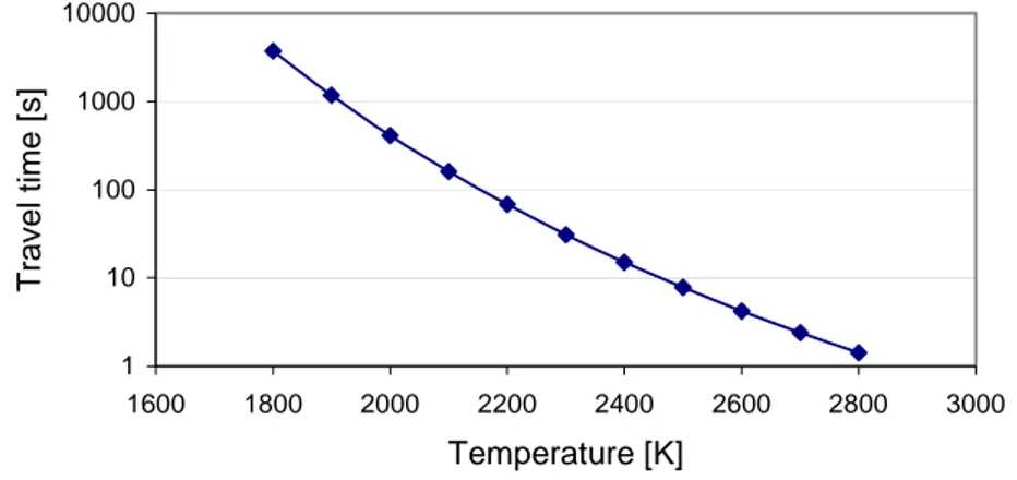
We have plotted the gas atom diffusion travel time versus temperature by substituting relation (2.27) for D in equation (2.31), figure 8. The results can be compared with figure 7b. As can be seen, at T=2200 K, t= 68 s compared to 1 s for the intra-granular bubble travel time. Thus, neglecting the gas atom diffusion during severe transients such as RIA is permissible. However, SCANAIR cannot be used to evaluate fission gas release during mild transients, such as ramp experiments that have been performed in the STUDSVIK and the RISØ reactors.

(a) 1.00E-08 1.00E-07 1.00E-06 1.00E-05 1.00E-04 1.00E-03 1600 1800 2000 2200 2400 2600 2800 3000 Temperature [K] Velocity [m/s] (b) 0.01 0.10 1.00 10.00 100.00 1600 1800 2000 2200 2400 2600 2800 3000 Temperature [K] Travel time [s]

Figure 7: Migration velocity and travel time of an intra-granular bubble in UO2 grain

as a function of temperature at a constant temperature gradient of ∂T/∂r= 400 K/mm during the transient. Grain radius of a=5 µm and bubble radius rib = 20 Å are assumed.

1 10 100 1000 10000 1600 1800 2000 2200 2400 2600 2800 3000 Temperature [K] Travel time [s]

3 SCANAIR interface: input and output data

SCANAIR is intended for modeling the thermal-mechanical fuel behavior under RIA, and does not comprise steady-state models for calculation of the fuel behavior prior to the transient. The base irradiation must therefore first be modeled by use of a steady-state fuel performance code, and the predicted fuel rod conditions transferred to the SCANAIR input deck, where they constitute initial conditions to the RIA. At present, the SCANAIR code has two pre-processor tools (TOSCAN and METEOSCAN) for convenient creation of SCANAIR input from output of the fuel rod analyses codes TOSURA and METEOR, respectively. The output from SCANAIR consists of

• A summary output file with primary fuel parameters in text format

• Binary warning messages on numerical problems and events encountered under calculation

• Several binary data files used for creation of graphs or alphanumeric tables

Post-processing tools are available for handling the binary output files, e.g. for plotting selected fuel rod parameters with respect to time or spatial position. In this section, we briefly review the input/output capabilities of the code. The full description of these capabilities and the input details are provided in the SCANAIR reference manual, Lamare (2001).

3.1 Input data to SCANAIR

The initial conditions for RIA analysis, i.e. the state of the fuel rod prior to an RIA, must be supplied from output of a general fuel rod thermal-mechanical code. At present, the SCANAIR code is designed to read such data from the codes TOSURA or METEOR via the interface programs TOSCAN and METEOSCAN. Through these interfaces, some data are read for the hot state of the fuel and others for the cold state. For the hot state, SCANAIR reads:

• End-of-life radial and axial fuel temperature profile • Radial and axial power profile

For the cold state, the following parameters are read • Fuel and clad radii and axial positions

• Radial distribution of plutonium concentration, burnup, stoichiometry, gas concentration, porosity and density of the fuel

• Gap gas components and concentrations

A calculation with SCANAIR is preferably initiated from cold state, since starting from a non-zero power may lead to differences between the hot state initial conditions calculated by SCANAIR and those from the pre-irradiation code (Lamare, 2001).

The input deck to SCANAIR is organized in blocks or structures, in which keywords are used for entering input parameters. The input syntax is clear and logical, and the syntactical correctness of all input data is checked by the SIGAL tool (Jacq, 1998). The default unit system for physical parameters is SI, but the pre-processor tool SIGAL handles most units. When departing from SI-units, the unit must be specified after the value entered in the input file. For example, 4.mm, will translate to 0.004 m. The list of main input structures in SCANAIR is shown in Table 3.1 below.

Table 3.1: Important input data structures to SCANAIR

Structure Task

TIME MANAGEMENT _{Time stepping and output instructions}

POWER _{Power history during transient}

FUEL _{Irradiated fuel material characterization}

CLAD _{Irradiated clad material characterization}

GAP _{Fuel-clad gap characterization}

MESHING AND GEOMETRY _{Meshing instructions for fuel and clad}

PHYSICAL PROPERTIES _{Material physical property data for fuel/clad}

FLUID _{Coolant properties}

WALL _{Thermal calculation of the shroud wall of the core}

BY-PASS _{Thermal outer boundary condition}

An important block in Table 3.1 is the STRUCTURE POWER, in which the power history during the transient and the power distribution profiles are defined. The axial and radial power profiles are assumed to be constant during the transient, and the relative power distribution is defined within the STRUCTURE POWER input block. The local power in a certain position is obtained by multiplying the relative power distribution with the total rod power at a given point in time. The total rod power as a function of time can be defined either as a simple time history table with power listed versus time, or in terms of the injected energy at a specific point in time. In the latter case, the radial average injected energy Einj [J/g] in the peak power axial segment at

time ts [s] is specified, together with a dimension-free time history f(t). The fuel rod

total power at time t is then defined through

) ( )

(t P f t

p = _T , (3.1)

where PT is calculated internally by SCANAIR through

∫

Here, mfuel is the fuel total mass, calculated from the input fuel density and volume, and

Z is the axial peaking factor. It should be noticed, that the power pulse shape f(t) is expected as input to SCANAIR, and must be based either on experimental data or calculations with an neutronics code.

3.2 Output data from SCANAIR

The output files created by SCANAIR are divided into 3 types

• A summary listing file with primary fuel parameters in text format

• Binary warning messages on numerical problems and events encountered under calculation

• Several binary data files used for creation of graphs or alphanumeric tables An event is defined as a transition from one state to another, e.g. closure of the pellet-clad gap in an axial segment. In the summary output, many detailed fuel and pellet-clad physical data are listed as a function of time and spatial position. Some data of particular interest for fuel and clad are stated in Table 3.2.

Table 3.2: Some quantities listed in SCANAIR summary output file listing.txt

Fuel Clad Radial temperature distribution Radial temperature distribution

Radial distribution of principal stresses Radial distribution of principal stresses Radial distribution of effective stress Radial distribution of effective stress Radial distribution of principal plastic

strains

Radial distribution of principal plastic strains

Radial distribution of principal elastic strains

Radial distribution of principal elastic strains

Radial distribution of thermal strains Radial distribution of thermal strains Plastic strain energy density 1 Plastic strain energy density 1

Enthalpy Swelling strain

Cracking strain

Fission gas concentration in fuel Gas bubble concentration

Gas bubble radii

Swelling of gas bubbles and pores Gas saturation of inter-granular bubbles

The summary output also includes the following quantities of interest, listed as functions of time. These quantities are either given for each axial segment of the rod or as rod averaged values:

• Average injected energy [J/g] • Average deposited energy [J/g] • Average enthalpy [J/g]

• Pellet clad contact pressure [Pa] • Free volume pressure [Pa] • Free volume gas composition • Rod average fission gas release

1

Plastic strain energy density is defined as: wpl =

∫

Various post-processing tools are available for handling the binary output files. As an example, for plotting selected fuel rod parameters with respect to time or spatial position, the SIGAL tool TIC is used. Although TIC seems to be an efficient graphic tool of general character, at Quantum Technologies, we have appended the general graphic tool X-manager to SCANAIR, since we have found it to be friendlier and more flexible to use.

4 Code implementation and documentation

4.1 Code implementation

The SCANAIR code is written in Fortran-77. The code makes extensive use of the utility program SIGAL, which is also written in Fortran-77, Jacq (1998). SIGAL is used for allocation, storage and handling of data structures, and also for pre- and post processing of data. The computational flow in SCANAIR is presented in figure 9.

Thermal computation Gas computation Mechanical computation Gas-mechanical update Output data Read input data Thermal-mechanical update Loop ov er time s tep s

The SCANAIR programming style in Fortran-77 is consistent and has good quality. It follows a set of programming rules regarding legibility, maintenance and portability. The code subroutines contain adequate amount of comments, which facilitate both maintenance and extension, Lamare and Latché (1995).

A drawback with SCANAIR in its present form, is that the code is tied to computers running POSIX-like operating systems, such as UNIX or Linux. The reason for this confinement is that the code and its pre- and post-processors are executed and controlled by use of shell scripts, written in the UNIX C-shell scripting language. At present, SCANAIR can thus not be run under the Microsoft Windows operating system.

4.2 Code documentation

The documentation related to SCANAIR is in general of good quality. At present, there are basically 3 documents describing the code and its use:

1. An original theory manual and model description, which was released together with version 2.2 of SCANAIR (Lamare and Latché, 1995).

2. A reference manual, accompanying version 2.3 of the code (Lamare, 1998). This document shortly describes modifications to the code introduced in version 2.3, and also provides a user’s manual with a description of input and output.

3. A reference manual, accompanying version 3.2 of the code (Lamare, 2001). This document shortly describes bug fixes and modifications to the code introduced in version 3.2, and also provides a completely revised user’s manual. The theory manual and model description to the present version of SCANAIR (3.2) is thus scattered over three different reports, which is inconvenient. A comprehensive document, describing the current state of the code, is therefore desirable.

The current user’s manual (Lamare, 2001) is well written, and together with examples of SCANAIR input files provided by IPSN, the code is comparatively easy to use. Documentation on verification and validation of the code is unfortunately weak; to our knowledge, there are no reports describing testing, verification and validation of the SCANAIR code, although some results of such work have been presented at international meetings and conferences, e.g. by Papin et al. (1997).

In addition to the documentation related directly to SCANAIR, there are also several documents describing the pre- and post-processors TOSCAN, METEOSCAN, and TIC. This is also true for the utility program SIGAL (Jacq, 1998).

5 Computations

Version 3.2 of the SCANAIR code was successfully installed in a Personal Computer (PC) environment, utilizing versions 7.0 and 7.1 of the Red Hat Linux operating system. A number of computations with SCANAIR were performed for the purpose of evaluation, verification and validation, and the results are presented in this chapter and relating appendices.

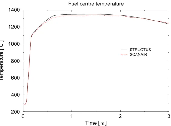
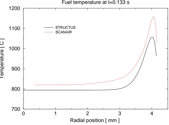
The verification computation is an RIA simulation test case, named REP4, which was provided to us by the developers of SCANAIR at IPSN/SEMAR in the Centre d’Etudes de Cadarache, France. The case was studied in detail and the results are documented in section 5.1 and appendix A. The rather extensive documentation of this case serves primarily for recognizing the capability of the code and its response, but it also serves as a well-documented reference case, which can be used to verify future code versions. Some of the SCANAIR results on the REP4 test case have also been compared with those obtained from calculations with the STRUCTUS code. The comparison, the results of which are presented in section 5.2, was made in order to independently verify the thermal-mechanical solution methods applied in SCANAIR.

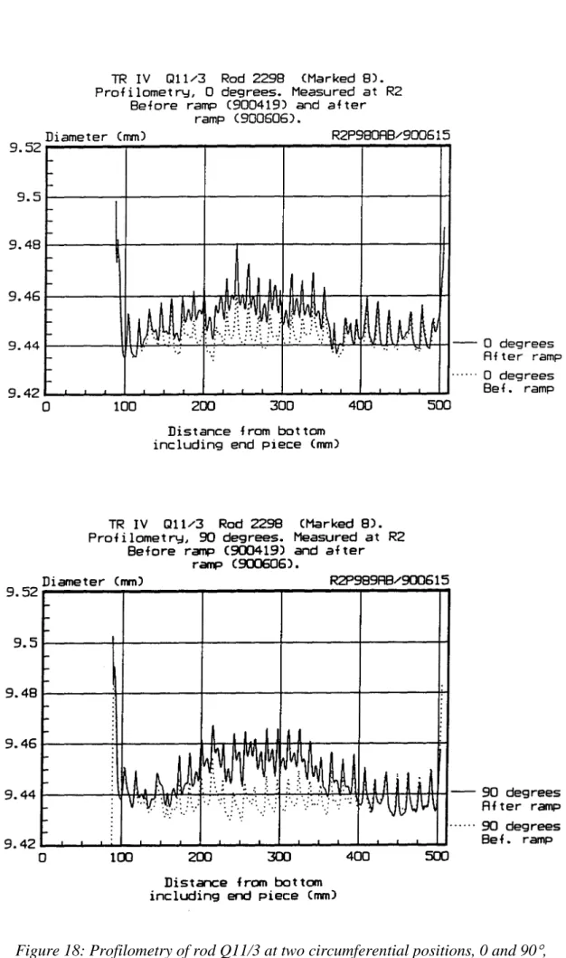
Next, SCANAIR was used to simulate a ramp test performed at Studsvik, namely, a test rod from the TRANS-RAMP IV project. Although SCANAIR is not designed to simulate such ramp experiments, we have applied it anyway, in order to get a realization of the limitation of the SCANAIR applicability. Results from this analysis are compared with experimental test data in section 5.3 and appendix B. Finally, a few SCANAIR results obtained from simulation of the test rod REP-Na2 are presented in section 5.4. The rod belongs to one of the RIA tests series, REP-Na, made in the French CABRI test reactor.

5.1 REP4 test case

The test case REP4 is a hypothetical transient case, used primarily for verification of SCANAIR installation and compilation. For us, it also functions as a reference test case, to which future versions of the code can be compared. Documentation of this test case is therefore important for the quality assurance of the code. Rod REP4 originates from a 17×17-array PWR rod, which has been pre-irradiated for 4 years. The segment of the rod that is subjected to a transient simulation had an average burnup of 7.44 atom%, corresponding to an exposure of about 69.5 MWd/kgU. The main data characterizing fuel rod dimensions and conditions prior to ramp are presented in Appendix A.

The pre-irradiation calculation was performed by IPSN, using the code TOSURA. In the pre-irradiation calculation, the rod was discretized by dividing it into three axial segments for both fuel and clad, 20 radial rings for the fuel, and six radial rings for the clad tube. The outermost ring of the tube represented the oxide layer. In the subsequent analysis with SCANAIR, each axial segment of the rod used in the pre-irradiation calculation was split into 4 segments. That is, the SCANAIR computation was performed for 12 axial segments. In addition, the fuel radial mesh in SCANAIR was extended to 28 rings, with a refinement in the fuel rim region.

0 0.1 0.2 0.3 0.4 0.5 0.6 0.7 0.8 0.9 1 Time [s] 0 10000 20000 30000

Linear power density [W/cm]

Peak linear power density, REP4

(a) 0.00 0.20 0.40 0.60 0.80 1.00 1.20 1.40 1 2 3 4 5 6 7 8 9 10 11 12 Axial segment Relative power bottom (b)

Figure 10: Transient power history for the test case REP4, (a) axial peak linear power density versus time, (b) axial power distribution, kept constant during the transient.

0 2 4 6 8 Time [s] 10 0 100 200 300 400 Deposited energy [J/g]

Averaged deposited energy, REP4

(a) 0 2 4 6 8 Time [s] 10 0 100 200 300 400 Enthalpy [J/g]

Fuel averaged enthalpy, REP4

(b)

Figure 11: Fuel rod axial peak radial average input energy quantities versus time during the transient, (a) deposited energy (absorbed heat), (b) enthalpy.

The transient power history that the fuel rod is subjected to is presented in figure 10a. The figure shows the peak linear power density, which corresponds to axial segment 7 from rod bottom; the constant axial power profile used throughout the transient is shown in figure 10b. The corresponding plots for the axial peak (i.e. segment 7) radial average deposited energy and enthalpy versus time are shown in figures 11a and 11b, respectively. In this transient simulation, the coolant is liquid sodium with inlet tempe-rature 281°C, inlet mass flow rate 0.308 kg/s, and a uniform pressure of 0.46 MPa.

Results:

The clad outer surface temperature and rod free volume pressure, calculated versus time by SCANAIR, are plotted in figures 12 and 13, respectively. Other output data of interest; relative power, plutonium concentration, burnup, fuel temperature, fuel swelling, as a function of fuel radius, are presented in appendix A. Also the calculated hoop plastic strain, hoop stress, and plastic strain energy density across clad are shown in appendix A.

Discussion:

The clad surface temperature, figure 12, reaches its peak value (352°C) at about 0.5 s from the start of the transient. Note that the linear power density reaches its peak at around 0.15 s, figure 10a. From figures 13a and 13b, we notice a substantial raise in rod internal pressure from 5.7 bar to 110 bar in a period of about 0.2 s, due to a rapid release of fission product gases. The fission gas content in the fuel porosity prior to the transient controls the gas release during the transient in SCANAIR. In input, the pore pressure (calculated by a steady-state fuel modeling code) is specified, and the van der Waals gas equation of state is then used in SCANAIR to calculate the associated fission gas content. The input pore pressure for the test case was 11.71 MPa.

0 2 4 6 8 Time [s] 10 280 300 320 340 360 Temperature [C]

Clad outer surface temperature, REP4

Figure12: Axial peak clad surface temperature versus time during the transient as calculated by SCANAIR.

0 2 4 6 8 Time [s] 10 0 50 100 150 Pressure [bar]

Rod free volume pressure, REP4

(a) 0.0 0.2 0.4 0.6 0.8 1.0 Time [s] 0 50 100 150 Pressure [bar]

Rod free volume pressure, REP4

(b)

Figure13: Rod internal pressure versus time during the transient, as calculated by SCANAIR at different time scales, 1 s and 10 s.