Real-time rendering of large terrains using algorithms for continuous level of detail

Real-time rendering of large terrains using

algorithms for continuous level of detail

(

HS-IDA-EA-02-103

)

Michael Andersson (a98mican@ida.his.se)

University of Skövde, Box 408 S-54128 Skövde, SWEDEN

Final Year Project in Computer Science, spring 2002. Supervisor: Mikael Thieme

[Real-time rendering of large terrains using algorithms for continuous level of detail]

Submitted by Michael Andersson to Högskolan Skövde as a dissertation for the

degree of B.Sc., in the Department of Computer Science.

[date]

I certify that all material in this dissertation, which is not my own work has been

identified and that no material is included for which a degree has previously been

conferred on me.

Real-time rendering of large terrains using algorithms for continuous level of

detail

Michael Andersson (a98mican@ida.his.se)

Summary

Three-dimensional computer graphics enjoys a wide range of applications of which games and movies are only few examples. By incorporating three-dimensional computer graphics in to a simulator the simulator is able to provide the operator with visual feedback during a simulation. Simulators come in many different flavors where flight and radar simulators are two types in which three-dimensional rendering of large terrains constitutes a central component.

Ericsson Microwave Systems (EMW) in Skövde is searching for an algorithm that (a) can handle terrain data that is larger than physical memory and (b) has an adjustable error metric that can be used to reduce terrain detail level if an increase in load on other critical parts of the system is observed. The aim of this paper is to identify and evaluate existing algorithms for terrain rendering in order to find those that meet EMW: s requirements. The objectives are to (i) perform a literature survey over existing algorithms, (ii) implement these algorithms and (iii) develop a test environment in which these algorithms can be evaluated form a performance perspective.

The literature survey revealed that the algorithm developed by Lindstrom and Pascucci (2001) is the only algorithm of those examined that succeeded to fulfill the requirements without modifications or extra software. This algorithm uses memory-mapped files to be able to handle terrain data larger that physical memory and focuses on how terrain data should be laid out on disk in order to minimize the number of page faults. Testing of this algorithm on specified test architecture show that the error metric used could be adjusted to effectively control the terrains level of detail leading to a substantial increase in performance. The results also reveal the need for both view frustum culling as well a level of detail algorithm to achieve fast display rates of large terrains. Further the results also show the importance of how terrain data is laid out on disk especially when physical memory is limited.

Table of contents

1

Introduction ... 1

2

Background ... 5

2.1 The three-dimensional graphics pipeline ...5

2.2 View frustum culling ...9

2.3 Level

of

detail...9

2.4 Algorithms...11

2.4.1 Real-time, continuous level of detail rendering of height fields ... 11

2.4.2 Real-time optimally adapting meshes ... 15

2.4.3 Real-Time generation of continuous levels of detail for height fields ... 18

2.4.4 A fast algorithm for large scale terrain walkthrough ... 20

2.4.5 Visualization of large terrains made easy... 21

3

Problem ... 25

3.1 Problem

definition ...25

3.2 Delimitation...25

3.3 Expected

result ...25

4

Method... 26

4.1 Test

architecture ...26

4.2 Test

cases ...26

5

Implementation ... 28

5.1 Algorithm

selection ...28

5.2 Memory

mapped

files ...28

5.3 Additional test cases ...29

5.3.1 File layout ... 29

5.3.2 Adjustable error metric ... 29

5.3.3 Terrain revisited... 29

5.3.4 Physical memory revisited ... 29

6

Results and analysis ... 30

7

Discussion ... 34

8

Conclusion ... 35

10

References... 37

11

Appendix A... 38

12

Appendix B... 39

1

Introduction

Three-dimensional graphics is something that most of us come in contact with in our

everyday life. Probably the most well know field of application for three-dimensional

graphics is in computer games where it is used to give the player a feel of depth and

realism. Back in 1991 Wolfenstein 3D (id Software, 1991) was released, a game with

great significance to the game industry. This was one of the fastest three-dimensional

games ever created for the personal computer and it marked the start of a new era in

the field of game development. A screenshot taken from this game is illustrated in

Figure 1.

Figure 1: Screenshot taken from Wolfenstein 3D.

Since then the computer game industry has flourished. The advances made in the area

of computer graphics hardware have given the programmer the ability to concentrate

on the development of even more stunning effects. More and more advanced games

are released every day incorporating network game play capabilities, advanced

physics and effects such as reflections and shadows to increase realism. An example

of such a game is Quake 3 (id Software, 1999) illustrated below in Figure 2.

Figure 2: Screenshot taken from Quake3.

Three-dimensional graphics also play an important role in applications used by

architects, engineers, artists, and others to create high quality images or accurate and

detailed technical illustrations. These are commonly referred to as Computer Aided

Design (CAD) applications and an example of such an application is illustrated in

Figure 3: Illustration of a model created with Design CAD 3D Max (Upperspace Coorp, 2001)

Those areas described so far are not its only range of applications. Three-dimensional

graphics also play an important role in different kinds of military simulators such as

radar and flight simulators (see Figure 4). In both these types of simulators

three-dimensional graphics is used to visualize the environment in which the simulation

takes place. One way to represent the environment is by using sampled terrain data,

which in conjunction with three-dimensional graphics can be used to render an image

of surroundings.

Figure 4: Screenshot from the Terra3D terrain engine (Wortham, 2002).

The three-dimensional terrain data used by these simulators can be represented in

several different ways. One common way is to use a rectangular grid of vertices

(elevation points) often referred to as a height field. An example of such a grid is

illustrated in Figure 5.

Figure 5: Terrain grid consisting of 9x9 vertices.

Simply illustrating the terrain in this way will not yield a satisfactory result. Some

geometric primitive is needed to connect the vertices constituting the terrain in order

to produce a continuous model. One common way to do this is by using triangles

since many graphics Application Programming Interfaces (API) and hardware

architectures are optimized for this geometric primitive (Möller & Haines 1999). An

example of how the vertices in the terrain grid in Figure 5 can be connected using

triangles is illustrated in Figure 6.

Figure 6: Illustration of a terrain grid where the elevation point has been connected using triangles.

The next step is to fill each triangle with colors based on the triangles orientation as

well as the orientation of the light sources. This gives the terrain a three-dimensional

effect and thereby resulting in a more realistic appearance. An example of how this

may look is illustrated in Figure 7.

Figure 7: Illustration of the model from Figure 6 with filled triangles.

Even though graphics hardware has come a long way, simply rendering all triangles in

a large terrain will bring even the latest hardware to its knees. An approximation of

the terrain is therefore needed to reduce the number of triangles used in the terrain

without compromising visual quality (Röttger, et al. 1998). These approximation

algorithms are refereed to as level of detail (LOD) algorithms. Such algorithms

perform on-the-fly approximation of the terrain where regions closer to the viewer as

well as regions with higher roughness is approximated using more triangles compared

to regions that are farther away or more flat. An example of how this may look is

illustrated in Figure 8.

Figure 8: Example of a terrain with decreased detail. The viewer is presumed to be located at the lower right corner.

Ericsson Microwave Systems (EMW) in Skövde develops simulators that with high

accuracy can reproduce radar functionality. EMW is looking for a terrain rendering

algorithms that meets the following requirements:

1.

The algorithm should be able to handle terrain data that is larger than main

memory of a single personal computer.

2.

The algorithm should be able to adjust the level of detail of the terrain if the load

on other relatively more critical parts of the system exceeds some threshold.

The aim of this paper is to identify and evaluate existing algorithms that conform to

EMW: s requirements. The objectives derived form this aim is to (i) perform a

litterateur survey over existing algorithms, (ii) implement the algorithms that meets

EMW: s requirements and (iii) develop a test environment in which these algorithms

can be evaluated from a performance perspective.

2

Background

This section begins with a description of the three-dimensional graphics pipeline of

which knowledge is important in order to understand the concepts related to

three-dimensional computer graphics as well as terrain rendering. This is followed by a

description of view-frustum culling in Section 2.2, a technique used to further

enhance performance by preventing non-visible geometry from being sent through the

pipeline. In Section 2.3 the concept behind level of detail algorithms will be

discussed. Such algorithms exploit the fact that parts of the terrain that are further

away from the viewer and/or more flat can be approximated using fewer triangles,

without compromising visual quality, compared to those regions that are closer and/or

more rough. Last, in Section 2.4 different continuous level of detail algorithms for

terrain rendering will be described in detail.

2.1

The three-dimensional graphics pipeline

The purpose of the three-dimensional graphics pipeline is to; given a virtual camera,

three-dimensional object, light sources, lighting models, textures and more render a

two-dimensional image (Möller & Haines 1999). Knowledge of the three-dimensional

graphics pipeline is fundamental in order to be able to understand the concepts of

three-dimensional terrain rendering. The purpose of this section is therefore to discuss

the pipeline and explain its different stages.

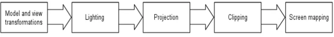
The pipeline, illustrated in Figure 9, is divided into three conceptual stages referred to

as the application, geometry and rasterizer stage (Möller & Haines 1999).

Figure 9: Illustration of the different stages of the graphics pipeline. Adapted from Möller and Haines (1999).

In the application stage, the developer has the ability to affect the performance of the

application. The reason for this is that this stage is always implemented in software,

which the developer is able to change. One purpose of this stage is to decrease the

amount of triangles to be rendered through different optimization techniques such as

view frustum culling (see Section 2.2). This stage is also the stage where processes

like collision detection, input devices handling etc. is implemented.

The second stage in the pipeline is the geometry stage, which is divided into the

functional steps illustrated in Figure 10.

Figure 10: Illustration of the different functional stages within the geometry stage. Adapted from Möller and Haines (1999).

The modeling and rendering of a cube will be used to explain these different stages.

First, the cube is created in its own local coordinate system also known as model

space as illustrated in Figure 11.

Figure 11: An illustration of the cube located in model space. The viewer is presumed to be looking down the negative y-axis. Adapted from Möller and Haines (1999).

The cube is associated with a set of model transformations, which affects the cube

position and orientation as illustrated in Figure 12, i.e. places the cube at the

appropriate position and orientation in the virtual world.

Figure 12: Illustration of the cube position, orientation and shape after the model transformations (a) rotation, (b) scaling, (c) translation, (d) all together. Adapted from Möller and Haines (1999).

In three-dimensional computer graphics the viewer’s position and view direction is

often described using a camera analogy. The camera is associated with the field of

view (FOV) as well as the near and far clipping planes. These properties define the

view volume, which is illustrated in Figure 13.

Figure 13: Illustration of the orientation, and the near and far clipping planes associated with the camera. Adapted from Möller and Haines (1999).

The goal is to render only those models that are within or intersect the camera’s view

volume. Therefore, in order to facilitate projection and clipping, a view

transformation is applied to the camera as well as the cube as illustrated in Figure 14.

Figure 14: The position and orientation of the camera and cube after view

transformation. The cameras view direction is now aligned with the negative z-axis. Adapted from Möller and Haines (1999).

After the view transformations the camera and the cube is said to reside in camera or

eye space in which projection and clipping operations are made simpler and faster

(Möller & Haines 1999).

The second functional step is the lighting step. The cube will not have a realistic feel

unless one or more light sources are added and therefore equations that approximate

real world lights are used to compute the color at each vertex of the cube. This

computation is performed using the properties and locations of the light sources as

well as the position, normal and material properties of the vertex. Later on when the

cube is to be rendered to the screen the colors at each vertex are interpolated over the

cubes surfaces, a technique know as the Gouraud shading (Möller & Haines, 1999).

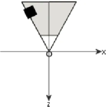
The next step is the projection step. In terrain rendering the most common type of

projection is called perspective projection in which the view volume is shaped like a

so-called frustum, a truncated pyramid with rectangular base. An illustration of the

frustum used in perspective projection is given in Figure 15.

Figure 15: Illustration of the view frustum used in perspective projection. As the figure illustrates the view frustum is shaped like a pyramid with its top cut off.

An important characteristic of this type of projection is that the cube will become

smaller as the distance between it and the camera increases. This result is exploited by

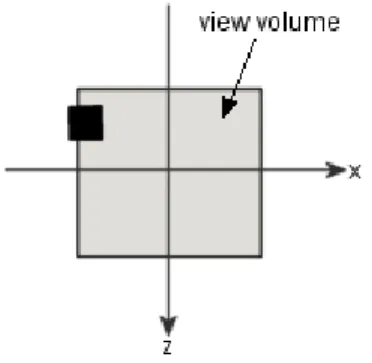
level of detail algorithms explained in Section 2.3. During projection the view volume

is translated and scaled into a unit cube with the dimensions x =

±

1, y =

±

1, z =

±

1

as illustrated in Figure 16. The reason for this is that clipping can be performed more

efficiently since vertices only have to be compared to the boundaries of the unit cube

(Möller & Haines, 1999).

Figure 16: The view volume shape and the cube position after projection. Adapted from Möller and Haines (1999).

The forth-functional step is the clipping step. Clipping is performed in order to reduce

the number of primitives being rendered to only those that is completely or partially

inside the view volume. Primitives that are completely inside the view volumes are

send to the next step directly whereas primitives that intersect the view volume needs

to be clipped before they are passed on. Clipping involves reducing the size of the

rendered cube to the one inside the view volume.

Figure 17: Illustration of the cube after the clipping stage. The size of the rendered cube is reduced to the one inside the view volume. Adapted from Möller and Haines (1999).

After the cube has passed through clipping it enters the fifth and final step referred to

as the screen-mapping step. Here the x and y coordinates of the points that the cube

consists of is transformed from their current unit cube format into screen coordinates.

The z-coordinate is not affected by this transformation.

The third stage in the three-dimensional graphics pipeline is the rasterizer stage. The

process performed in this stage known as rasterization or scan conversion involves

conversion of the cube and its colors into pixels on the screen. The rasterizer stage is

also the stage where texturing is performed. Texturing essentially means to glue an

image onto an object, which further leads to an enhancement of visual appearance.

2.2

View frustum culling

Rendering performance can be improved by applying view-frustum culling of

bounding volumes during the application stage of the pipeline (Assarsson & Möller

2000). This way non-visible geometry can be discarded early in the process leading to

a reduced number of primitives sent through the rendering pipeline. Instead of testing

every object against the view-frustum a bounding volume is used to group a set of

object together inside an enclosing volume, as illustrated in Figure 18. A simple

intersection test between the bounding volume and the view-frustum can be used to

determine whether the objects inside the volume are visible or not.

Figure 18: Illustration of two triangles contained within an oriented bounding box.

According to Möller and Haines (1999) the most common types of bounding volumes

is spheres, axis aligned bounding boxes (AABB’s) and oriented bounding boxes

(OBB’s).

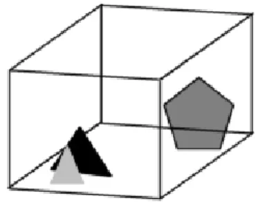
Organizing the bounding volumes in a hierarchy, for example a tree, leads to another

beneficial fact. If the bounding volume of a parent node is not visible then its children

cannot be visible since these are completely contained within the parent. This leads to

an even faster reduction of non-visible geometry as well as an increase of

performance since less bounding volumes has to be tested for intersection with the

view frustum. An example of a hierarchy of bounding volumes is illustrated in Figure

19.

Figure 19: Illustration of how the original volume that contains two triangles and a pentagon is organized into a hierarchy of bounding volumes. If the parent isn’t visible then neither is the children.

2.3

Level of detail

Even though large parts of the terrain and other object in the virtual world can be

discarded through hierarchical view-frustum culling brute force rendering of the

remaining parts of the terrain will still not result in interactive frame rates. Lindstrom

and Pascucci (2001) argue that it is essential to perform on-the-fly simplification of a

high-resolution mesh in order to accommodate fast display rates. This simplification

process is commonly refereed to level of detail (LOD). LOD exploits the fact that

when the distance from a model to the viewpoint increases the model can be

approximated with a simpler version, without compromising visual quality. The

reason that visual quality is not compromised is because of the main characteristic of

perspective projection, explained in Section 2.1, which states that an object will be

smaller as it gets further way from the viewpoint thus covering a less area of pixels.

The simplest type of LOD is discrete LOD (DLOD) (Möller & Haines 1999), which

uses different models of the same object where each model is an approximation of the

original object using fewer primitives. Switching between detail levels is done when

the distance from the viewpoint to the object is greater or equal to that levels

associated threshold value. Using this type of LOD a switch during rendering often

produces a noticeable and not visually appealing “popping effect” when the level of

detail suddenly is decreased (Ederly 2001). An example of the work of a DLOD

algorithm is illustrated in Figure 20.

Figure 20: Illustration of three different discrete levels of detail. As the viewer moves further away form or closer to the terrain a switch between these levels of detail is conducted.

When working with terrain rendering DLOD can be applied to small parts of the

terrain, know as blocks instead of the entire terrain. An example of a terrain rendered

with block DLOD is illustrated in Figure 8.

Another type of LOD is continuous LOD (CLOD), which is based on dynamic

triangulation of the model where a small amount of triangles are changed at a time

(Röttger, et al. 1998; Ederly 2001). The advantage of using CLOD instead of DLOD

is that, since CLOD only removes a small number of triangles, the popping effect

becomes less noticeable. The reduced level of detail produced by a CLOD algorithm

is illustrated below in Figure 21.

Figure 21: Illustration of the work performed by a continuous level of detail algorithm. As the viewer moves further away from lower right corner of the terrain the detail level is slowly reduced.

A problem that often occurs when using the block DLOD and CLOD methods in

terrain rendering is the occurrence of cracks between adjacent terrain blocks with

different levels of detail. These cracks causes’ unwanted holes resulting in a

non-continuous terrain as illustrated in Figure 22.

Figure 22: Illustration of cracks between adjacent terrain blocks with different levels of detail. Adapted from Youbing (2001).

The solution to this problem is algorithm specific since it depends on how the

algorithm performs terrain triangulation. Some of the existing algorithms for terrain

rendering and how they solve this problem among other things will be discussed in

the next section.

2.4

Algorithms

This section describes five different continuous level of detail algorithms for terrain

rendering. The purpose of this section is not to serve as a verification of the

correctness of these algorithms but as a summary of their central components.

2.4.1

Real-time, continuous level of detail rendering of height fields

The algorithm for terrain rendering presented by Lindstrom et al. (1996) is based on

simplification instead of refinement, which is the approach taken by the other

algorithms described in this paper. The terrain is divided into blocks with the fixed

dimensions 2n+1 surrounded by an axis-aligned bounding block used for view

frustum culling as well as discrete level of detail (see Section 2.3) computations.

These blocks are subjects for a fine-grained as well as a course-grained simplification

step. In the fine-grained simplification step recursive simplification of the terrain is

performed by merging triangles pairs al, ar into al

⊕ar if the right conditions are meet

as illustrated in Figure 23.

Figure 23: Illustration of the merging process of the triangles al and ar. After merging the two original triangles al and ar are reduced to a single triangle al⊕ar.

The merging condition states that two triangles should be merged if and only if the

length of the delta segment

δ when projected onto the projection plane is smaller than

the threshold

τ. Here projection aims at the process of mapping a point p= (px, py, pz)

onto a plane z = -d, d > 0 resulting in a new point q= (qx, qy, -d) (Möller and Haines,

1999) as illustrated in Figure 24.

Figure 24: Illustration of projection of p onto the plane z = -d. The viewer is presumed to be looking down the x-axis. Adapted from Möller and Haines (1999)

The similar triangles can be used to derive the y component of q as follows in

equation ( 1 ):

p

p

d

q

p

d

p

q

−

=

⇔

−

=

( 1 )

The

x component of q can be derived in a similar manner. Equation ( 1 ) is actually

the basis for perspective projection and as explained in Section 2.1, perspective

projection has the characteristic that an object becomes smaller as the view moves

away from it and thus it covers a smaller region of the screen. The same goes for the

projected delta segment, which is illustrated in Figure 25.

The length of the delta segment in screen space, illustrated in Figure 25, can be

computed by using equation ( 2 ):

2 2 2 2 2

)

(

)

(

)

(

)

(

)

(

v

e

v

e

v

e

v

e

v

e

d

−

+

−

+

−

−

+

−

=

λδ

δ

(

2

)

In the equation above e is the viewpoint, d is the distance form the viewpoint to the

projection plane and

λ is the number of pixels per world coordinate unit in the screen

space coordinate system. By rearranging equation ( 2 ) the computational expensive

square root can now be eliminated and the simplification condition can be rewritten as

follows:

)

)

(

)

(

)

((

)

)

(

)

((

e

−

v

+

e

−

v

≤

K

e

−

v

+

e

−

v

+

e

−

v

δ

In the inequality above K=

τ

/(d

λ

) and hence adjusting the error threshold

τ

will result

in an increased/decreased level of detail.

Simply evaluating this fine-grained simplification condition for all vertices within a

certain block each frame will be too computational expensive. Therefore a

course-grained simplification step is introduced in which a discrete level of detail is selected

(see Section 2.3). By using maximum delta value,

δ

_{max, computed from the lowest}

level vertices for each block and the axis-aligned bounding box one can for a given

viewpoint determine whether any of these vertices have delta values large enough to

exceed

τ. If

δ

_{l denotes the lowest delta value that when projected can exceed τ and}

δ

_h

denotes the largest delta value that may project smaller than

τ, vertices with delta

values that fall between these two extremes defining the so called uncertainty interval

Iu, will have to be evaluated using equation ( 2 ). A vertex can be discarded from the

resulting mesh if its delta value is less than

δ

_{l. Conversely a vertex cannot be removed}

if its delta value is larger than

δ

_h.

To compute

δ

_{l the maximum value of the following function must be found:}

2 2 2 2 2 2 2

₍

₎

₍

₎

₍

₎

)

(

)

(

)

,

(

v

e

v

e

v

e

v

e

v

e

h

r

r

h

r

f

−

+

−

+

−

−

+

−

=

+

=

This function is constrained by

r

+

h

≥

d

and

v

∈ where B is the set of points

B

contained with in the bounding box. The two vectors describing this bounding box are

)

(

)

(

b

b

b

b

b

b

b

b

=

=

Let rmin be the smallest value distance from

[

e

e

]

to the rectangular region of the

bounding box defined by

[

b

b

]

⎪⎭

⎪

⎬

⎫

⎪⎩

⎪

⎨

⎧

>

<

=

otherwise

x

x

x

if

x

x

x

if

x

x

x

x

clamp

min min max min

,

,

)

(

By setting

|

)

,

,

(

|

e

clamp

b

e

b

h

h

=

=

−

the maximum value fmax of f(r, h) is found at r=h. If no vertex v exists under the

given constraint that satisfies r=h then r is increased/decreased until

v

∈ . In other

B

words

r

=

clamp

(

r

,

h

,

r

)

.

In contrast to maximizing the function f(r, h) in order to find

δ

_{l the same function has}

to be minimized to find

δ

_{h. By setting}

|}

|

|,

max{|

max

e

b

e

b

h

h

=

=

−

−

fmin can be found either when r=rmin or r=rmax, whichever yields a smaller f(r, h).

The bounds on Iu can now be found using equations ( 3 ) and ( 4 ):

max

f

d

λ

τ

δ =

( 3 )

⎪

⎪

⎩

⎪

⎪

⎨

⎧

∞

>

>

=

=

otherwise

f

and

if

f

d

if

0

0

0

0

τ

λ

τ

τ

δ

( 4 )

By recursively comparing whether

δmax<δl the current block is substituted by a lower

resolution level of detail block. If on the other hand

δmax>δl it may be that a higher

resolution block is needed.

Simply applying the fine-grained and course-grained steps described above will result

unwanted cracks (see Section 2.3) occurring between blocks as well as inside them.

The reason for this is that there exists dependencies between vertices that aren’t

fulfilled and therefore cracks are introduced. An illustration of the vertex

dependencies is given in Figure 26.

Figure 26: Illustration of the vertex dependencies. An arrow from A to B indicates that B depends on A. Adapted from Lindstrom et al. (1996)

The merging of a triangle pair is only possible if the triangle pair appears on the same

level in the triangle subdivision. The process of merging triangles can be viewed as

the removal of the common base vertex as illustrated below in Figure 27.

Figure 27: Illustration of the merging process by base vertex removal. After merging the original four triangles are reduced to two triangles.

The mapping of vertices to triangle pairs results in a vertex tree where each node,

except for the root and leaves as well as the vertices on the edges of the block, has

two parents and four decedents. If any of the decedents of a vertex v is included in the

rendered mesh, so is v. In other words v is said to be enabled. To solve the occurrence

of cracks between adjacent blocks vertices may be labeled as locked. The result of

this is that vertices on the boundaries of the higher resolution block may have to be

permanently disabled during simplification.

As with all block-based algorithms extra software can be used to support terrains

larger than main memory. This is done by paging blocks in and out of memory when

needed/not needed by the algorithm. Lindstrom et al. (1996) describes no such

mechanism.

2.4.2

Real-time optimally adapting meshes

The Real-time optimally adapting meshes (ROAM) presented by Duchaineau et al.

(1997) is an algorithm that since its publication in 1997 has been widely used in

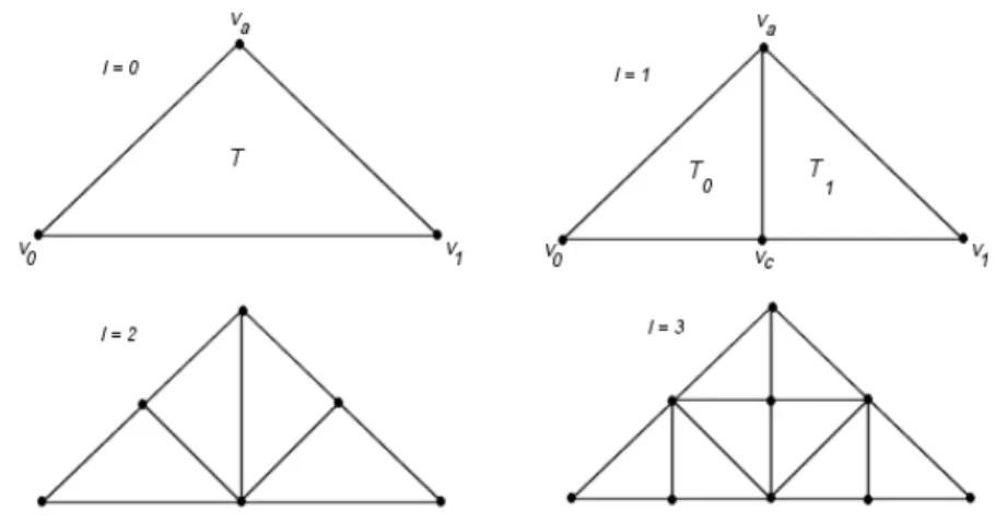
games (Youbing et al. 2001). In this algorithm the triangle bintree structure

constitutes the central component of which the first few levels are illustrated in Figure

28.

Figure 28: Illustration of the levels 0-3 of a triangle bintree. Adapted from Duchaineau et al. (1997)

In Figure 28 T denotes the root triangle which is a right-isosceles triangle at the

coarsest level of subdivision. A right isosceles triangle is a triangle where two of the

interior angles are equivalent and the third equals 90o. In order to produce the

next-finest level of the bintree the root triangle T is split into two smaller child triangles

(T0, T1) separated by the edge stretching form the root triangle’s apex va to the center

vc of its base edge (v0, v1). To produce the rest of the triangle bintree this process is

repeated recursively until the finest level of detail is reached.

Changing of a bintree triangulation can be performed using two different operations,

split and merge. The consequence of using these operations is illustrated in Figure 29.

Figure 29: Illustration of the result produced by the split and merge operations respectively. Adapted from Duchaineau et al. (1997).

As illustrated above the split operation replaces a triangle T with its children (T0, T1),

and TB with (TB0, TB1). Figure 29 also illustrates the relationship between the

triangles in the neighborhood of T where TB is the base neighbor of T and TL and TR

are the left- and right neighbors respectively. Another important fact about triangle

bintrees that also is show in Figure 29 is that the neighbors are either from the same

bintree level l as T, or from the next finer level l+1 for the left and right neighbors, or

from the next courser level l-1 for the base neighbor. If the triangles T and TB are

from the same bintree level they are said to form a diamond.

If cracks are to be prevented from occurring between neighboring triangles a triangle

T cannot be split directly if its base neighbor TB is from a courser level. Therefore the

base neighbor TB must be forced to split before T. As illustrated in Figure 30 the

forced split of the base neighbor TB may trigger forced splitting of other triangles.

Figure 30: Illustration of the concept of forced splitting. The splitting of the triangle T triggers a series of forced splits starting at TB and ending with a split of the two largest triangles. Adapted from Duchaineau et al. (1997).

To drive the split and merge operations the algorithm utilizes two priority queues, one

for each operation. The content of these queues are the triangles, ordered by priority

that needs to be split or merged respectively. The advantage of using a second priority

queue for mergable diamonds is that it enables the algorithm to exploit

frame-to-frame coherence by allowing the algorithm to start from a previously optimal

triangulation.

In order to make the algorithm work properly the priorities must be monotonic which

means that a child’s priority cannot be large that its parents. To compute the queue

priorities a bound per triangle must be used. An example of such a bound is a wedgie

(illustrated in Figure 31), defined as the volume of world space containing points (x,

y, z) such that (x, y)

∈ T and |z-zT(x, y)| ≤ eT for some wedgie thickness eT.

Figure 31: Illustration of a pair of triangles and the bounding wedgie in which they are contained.

The nested wedgie thickness can now be computed in a bottom-up fashion as follows:

⎩

⎨

⎧

−

+

=

otherwise

|

)

(

)

(

|

)

,

max(

level

finest

at the

0

v

z

v

z

e

e

e

Using the wedgie thickness the screen space error that also is the triangles priority can

be computed using equation ( 5 ):

|

,

|

)

(

c

r

b

q

c

r

b

q

c

r

a

p

c

r

a

p

v

dist

−

−

−

+

+

−

−

−

+

+

=

( 5 )

In equation ( 5 ) above (p, q, r) are the camera space coordinates of the vertex v and

(a, b, c) is the camera space vector corresponding to the world-space thickness vector

(0, 0, eT). Equation ( 5 ) can be rewritten as illustrated in equation ( 6 ):

2 1 2 2 2 2

((

)

(

)

)

2

)

(

ar

cp

br

cq

c

r

v

dist

−

+

−

−

=

( 6 )

Hence a triangles priority increases with the size of the projected error.

In the introduction of this paper the Duchaineau et al. (1997) explain that a complete

system for terrain rendering consists of, among other things, a component to manage

disk paging of terrain geometry. Even so no such mechanism is presented and in the

conclusion the authors state that this is a critical issue that remains to be solved.

2.4.3

Real-Time generation of continuous levels of detail for height fields

The algorithm presented by Röttger et al. (1998) is based on the hierarchical quadtree

(a tree in which each node has four children) technique introduced by Lindstrom, et

al. (1996). In contrast to the approach taken by Lindstrom, et al. (1996) this algorithm

uses a top-down refinement strategy instead of a bottom-up strategy, which resulted in

higher performance since only a fraction of the nodes in the height field is visited

each frame. The height field is assumed to be of the size 2n+1x2n+1 and a boolean

matrix, in which each entry indicates whether the node is used in the terrain or not as

well as if it is an internal node or a leaf, represents the quadtree used to traverse the

vertices in the terrain. An example of a terrain produced by this algorithm along with

its boolean quadtree matrix is illustrated in Figure 32.

Figure 32: An example of a 9 x 9 terrain produced by this algorithm along with its boolean quadtree matrix representation. Internal nodes in the tree are marked with a 1, leafs are marked with a 0 and entries marked with a ? are not parts of the rendered terrain. Adapted from Röttger et al. (1998).

In order to render the terrain the quadtree is traversed recursively and when a leaf is

reached a full or partial triangle fan is rendered. A triangle fan is a set of connected

vertices where each triangle shares the center vertex. Triangle fans are a compact way

to describe triangles resulting in fewer vertices being sent to the rendering pipeline

compared to usual method to describe triangles. An example of a triangle fan is

illustrated below in Figure 33.

Figure 33: Illustration of a triangle fan, the primary geometric primitive used for rendering of the quadtree leaves.

In Figure 33 the starting triangle sends vertices v0, v1 and v2 (in that order) but for the

following triangles only the next vertex, in this case v3, is sent since it is being used

together with the center vertex as well as the previously sent vertex to from a new

triangle.

Using this method as is would result in cracks occurring between adjacent blocks of

different detail levels (se Section 2.3). Simply skipping the center vertex at these

edges prevents this (Röttger et al, 1998). In order for this technique to work the

difference in detail level between adjacent blocks can be at most one. How this is

solved will be explained shortly.

When performing the refinement step of the algorithm the following two criterions

need to be fulfilled. First, the level of detail should decrease as the distance to the

viewpoint increases. Second, the level of detail should be higher for regions with high

surface roughness. These criterions are in compliance with the description of LOD in

Section 2.3. The surface roughness can be pre-calculated using equation ( 7 ):

|

|

max

1

2

dh

d

d

=

( 7 )

In the equation above d is the edge length of the block and dhi is the absolute value of

the elevation difference as show in Figure 34:

Figure 34: Illustration of how the surface roughness is measured. Adapted from Röttger et al. (1998)

Using equation ( 7 ) Röttger, et al. (1998) presents the subdivision criterion stated in

equation ( 8 ):

1

)

1

,

2

*

max(

*

*

<

=

refine

if

f

d

c

C

d

l

f

( 8 )

Here l is the distance to the viewpoint, C is the minimum global level of detail and c

is the desired global level of detail, which can be used to adjust the level of detail. In

order to impose the requirement that the difference in level of detail between adjacent

blocks cannot be larger than 1 for the crack prevention technique explained earlier to

work the pre-calculation of the d2-values must be performed in the following manner.

Calculate the local d2-values of all blocks and propagate them up the tree, starting at

the smallest existing block. The d2-value of each block is the maximum of the local

value and K times the previously calculated values of adjacent blocks at the next

lower level. The constant K can be calculated using the minimum global level of

detail as stated in equation ( 9 ):

)

1

(

2

−

=

C

C

K

( 9 )

In order to be able to render terrains that do not entirely fit into main memory Röttger

et al. (1998) explain the need of an explicit paging mechanism but no such

mechanism is presented.

2.4.4

A fast algorithm for large scale terrain walkthrough

The algorithm presented by Youbing et al. (2001) is based on regular grids as well as

the division of large terrains into smaller blocks and it implements a very simple and

fast way to prevent cracks between different levels of detail. One common way to

perform crack prevention in algorithms based on top-down refinement such as this

one is by recursively splitting of neighborhood triangles (see Figure 35). Recursive

splitting has the disadvantage of introducing unnecessary triangles and instead this

algorithm simply alters the elevation of the vertex that is on the crack as illustrated in

Figure 35. The disadvantage of this method is that it causes so-called T-junctions

because of the floating-point inaccuracy, which results in a noticeable “missing

pixels” effect.

Figure 35: Illustration of two different approaches to crack prevention. On the left cracks are prevented through recursive splitting and on the right through elevation alternation. Adapted from Youbing et al. (2001)

The refinement method used in this algorithm is a hybrid of the block based quad

subdivision method used by Lindstrom et al. (1996) and the right isosceles based

binary subdivision used by Duchaineau et al. (1997). This hybrid method starts by

dividing the initial block into two right isosceles, which are then further recursively

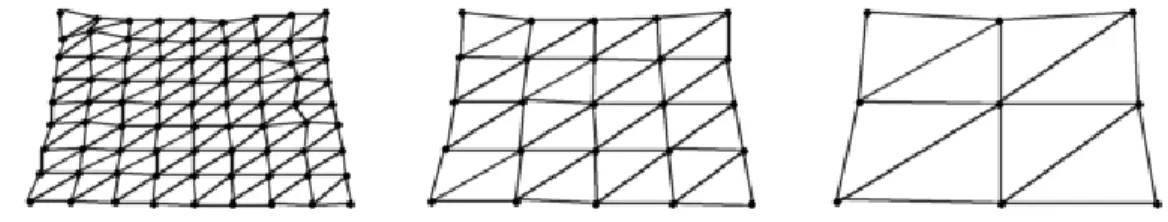
quad subdivided, based on screen space error metric.

Figure 36: Illustration of the first steps of the subdivision process. The left illustration shows the split of a block into two right isosceles and the middle and right illustrations shows the first recursive quad subdivision process.

The authors explain that even though their algorithm can handle relatively large

terrains they are still limited to the amount of physical memory. Therefore an explicit

mechanism for paging of terrain blocks or compression is needed but none of these

mechanisms is presented.

2.4.5

Visualization of large terrains made easy

The algorithm presented by Lindstrom and Pascucci (2001) diverge a bit form the

common approach as instead of focusing on how to divide a large terrain into blocks

that eventually could be paged in and out of main memory by an explicit paging

mechanism Lindstrom and Pascucci (2001) simply delegates the task of paging terrain

data to the operating system by using memory mapped files. As a result focus is laid

on how to organize the file on disk in order to improve coherency for a given access

pattern. Such algorithms, aimed at solving issues related to the hierarchical nature of a

modern computers memory structure, are commonly referred to as external memory

algorithms or out-of-core algorithms.

For terrain refinement Lindstrom and Pascucci (2001) choose the top-down approach

subdividing the terrain, constrained to 2n/2+1 vertices in each direction where n is the

number of refinement levels, using the longest edge bisection scheme where an right

isosceles triangle is refined by bisecting its hypotenuse resulting in two smaller right

triangles as illustrated in Figure 37.

Figure 37: Illustration of the edge bisection hierarchy. The arrows symbolize the parent-child relationships in the directed acyclic graph of the mesh vertices. Adapted from Lindstrom & Pascucci (2001)

The triangle mesh produced by this bisection scheme can be viewed as a directed

acyclic graph where an edge (i, j) represents a bisection of a triangle where j is

inserted on the hypoteneous and connected to i at the right angle corner of the

triangle. In order to produce a continuous terrain without T-junctions and cracks the

following properties must be satisfied:

M

i

M

j

∈

⇒

∈

j

∈

C

Here M represents a given refinement and Ci is the set of children of i. This property

implies that if an elevation point j is active so must its parent. To ensure the

satisfaction of this property the following condition must apply:

)

,

,

(

)

,

,

(

δ

p

e

ρ

δ

p

e

ρ

≥

∀

j

∈

C

In the condition above

ρ is the projected screen space error term, pi is the position of

the vertex i,

δi is an object space error term for i and e is the viewpoint. Hence ρ

consists of two different parts, which are the object space error term,

δi and a

view-dependent term that relates pi and e. As mentioned above the error terms must be

nested to guarantee that a parent is active if any of its children is active. Nesting of the

object space error term

δi can therefore be calculated in the following manner:

⎪⎩

⎪

⎨

⎧

=

max{

,

max{

}}

δ

δ

δ

δ

This does not guarantee

ρ(δi*, pi, e) ≥ ρ(δj*, pj, e) for j ∈ Ci because the viewer

might be close to the child pj and far from parent pi. To solve this Lindstrom and

Pascucci (2001) uses a nested hierarchy of nested spheres by defining a ball Bi of

radius ri centered on pi where ri is calculated in the following manner:

⎪⎩

⎪

⎨

⎧

+

−

=

{|

|

}

max

0

_p

_p

_r

r

The adjusted projected error can now be written as

)

,

,

(

max

e

x

δ

ρ

ρ

=

It is important to mention that this is the general framework for refinement and that

the algorithm is virtual independent of the error metric being used. Even so Lindstrom

and Pascucci (2001) describe the projected error metric used by their terrain

visualization system, which is stated in equation ( 10 ) :

i i i i

r

e

p

−

−

=

|

|

λ

δ

ρ

( 10 )

In equation ( 10 ) above

λ

=w/

ϕ

where w is the number of pixels along the field of

view

ϕ, pi is the vertex being evaluated, e is the viewpoint and ri is the radius of the

if i is a leaf node

otherwise

if i is a leaf node

otherwise

sphere centered at pi. Now

ρ

can be compared against the screen space error

tolerance

τ to find out whether an elevation point i should be active or not.

As mentioned briefly in the beginning of this section the algorithm delegates the task

of paging terrain data to the operating system and instead focuses on how the terrain

data should be laid out on disk in order to minimize paging events. In order to achieve

this Lindstrom and Pascucci (2001) argues that vertices that are geometrically close

should be stored close together in memory to achieve good memory coherency. To

preserve these neighborhood properties the authors introduced the concept of

interleaved quadtrees where vertices are labeled as white or black depending on

whether they are introduced at an odd level or an even level respectively. An

illustration of the white and black quadtrees is illustrated in Figure 38.

Figure 38: Illustration of the first three levels of the white and black quadtree respectively. Adapted from Lindstrom & Pascucci (2001)

In Figure 38 above vertices outside of the rectangular grid are marked with cross

indicating that these are so-called ghost vertices. When the terrain is stored linearly on

disk the ghost vertices will produce “holes” in the array thus leading a waste of disk

space.

Lindstrom and Pascucci (2001) also describe the importance of efficient index

computations in order not to impose any overhead during the refinement of the

terrain. If the terrain data is not stored as interleaved quadtrees but simply in linear

order the index computations can be performed using equation ( 11 ):

2

v

v

v

=

+

( 11 )

In equation ( 11 ) above vm is the center vertex of the edge connecting the two

triangle corners vl and vr as illustrated in Figure 39. On the other hand, if the

interleaved quadtree approach is used equation ( 12 ) states how to perform index

computations:

m

m

p

p

p

p

p

c

m

m

p

p

p

p

p

c

+

+

+

+

+

=

+

+

+

+

+

=

)

4

mod

)

2

2

((

4

)

,

(

)

4

mod

)

1

2

((

4

)

,

(

( 12 )

In the equations above m is a constant dependent of the index of the root node and the

index distance between consecutive levels of resolution. An illustration of geometric

meaning of the variables used in both the equations above is shown in Figure 39.

Figure 39: Illustration of the geometric meaning of the variables used by the index computation equations. Adapted from Lindstrom & Pascucci (2001)

To conclude this discussion about terrain data layout and efficient index computation

an example of the indices of the first few levels of the white and black quadtrees is

illustrated in Figure 40.

Figure 40: Illustration of the indices for the first few levels of the white and black quadtrees. Adapted form Lindstrom & Pascucci (2002).

3

Problem

Ericsson Microwave Systems (EMW) in Skövde, a member of the Ericsson group

provides a professional competence as well as resource reinforcement in the field of

software engineering. A part of EMW: s activity is to develop simulators that with

high accuracy can reproduce radar functionality. In order to evaluate the results of a

simulation, manual analysis of tables of simulation data is conducted a tedious

process for large simulations. Therefore EMW seek to incorporate three-dimensional

graphics into their simulators to extend these with the ability to provide the operator

with visual feedback during a simulation.

In these simulators it is important to be able to verify the surrounding environment,

consisting of three-dimensional terrain data, in which the simulation takes place.

EMW is looking for a terrain-rendering algorithm that meets the following

requirements.

1.

The algorithm should be able to handle terrain data that is larger than main

memory of a single personal computer.

2.

The algorithm should be able to adjust the level of detail of the terrain if the load

on other relatively more critical parts of the system exceeds some threshold.

The latter requirement is important since, even though terrain rendering constitutes a

central component of these simulators, it is important that the simulator’s performance

is not compromised because of the complex surroundings. The increase in system

load can be due to an increase in the number of targets entering the simulations.

3.1

Problem definition

A lot of different algorithms for terrain rendering have been developed during the last

decades all with their own set of pros and cons. The aim of this paper is to identify

and evaluate those algorithms that conform to EMW: s requirements. This aim is

broken down into the following objectives to (i) perform a litterateur survey over

existing algorithms in order to find those algorithms that fit EMW: s needs, (ii) to

implement these algorithms and (iii) develop a test environment in which these

algorithms can be evaluated from a performance perspective.

3.2

Delimitation

My work is solely concentrated on finding those algorithms that best satisfies EMW: s

requirements, to implement and evaluate these algorithms from a performance

perspective. The algorithms should be able to meet the requirements “as is” without

modification as well as extra functionality.

3.3

Expected result

My expectation is to find at least one algorithm that will meet EMW: s requirements

and I expect to be able to show that this or these algorithms will have a positive

impact on EMW: s simulators.

4

Method

To evaluate the performance of the algorithms tests will be conducted on a specified

test architecture using combinations of test cases designed to measure the algorithm

performance. The configuration of the test architecture is explained in Section 4.1 and

the different test cases will be stated in Section 4.2

4.1

Test architecture

The test architecture used for testing of the algorithms is constituted by a Dell

Optiplex GX240 equipped with a Intel Pentium 4 1.8 GHz processor, 513 MB RAM,

36 GB IDE HD and a Hercules 3D Prophet II Geforce 2 GTS Pro 64MB graphics

card. The operating system running on this machine is Mandrake Linux version 8.0

and it uses OpenGL, an application programming interface (API) developed by SGI in

1992, for rendering as well as the OpenGL Utility Toolkit (GLUT), a simple

windowing API for window management. The compiler used by the test architecture

is the GNU Compiler Collection (GCC) version 2.96 and common to all tests is the

window size of 800x600 pixels as well as 60 degrees field-of-view (see Section2.1).

4.2

Test cases

The following sections describe the different test cases that will be used to test the

performance of the algorithms. In Section 4.2.1 the terrain used through all test cases

is described followed by a description of the fly-over path in Section 4.2.2. Section

4.2.3 discusses the four different operations that will be tested and Section 4.2.4 deals

with the test case involving different memory configurations.

4.2.1

Terrain

The terrain used to test the algorithms is the one used by Lindstrom and Pascucci

(2001). This terrain, a subset of the original terrain provided by The United States

Geological Survey (USGS), with the dimensions 16385x16385 pixels uses an

inter-pixel spacing of 10 meters as well as maximum height of 6553.5 meters. The

motivation for using this terrain is that in contains both flat and rough regions, which

when flown over will provide results on how dependent the algorithm performance is

of the underlying terrain complexity. The terrain is illustrated in Section 11.

4.2.2

Path

When flying over the terrain a similar path is taken through all test cases. By attaching

the camera onto a mathematical curve called a Hermite spline (named after the Frence

mathematician Charles Hermite) a terrain fly-over can be performed. The path is

formed like a double eight and it constitutes a good fly-over path as it passes over

both rough and flat regions of the terrain. The fly-over path is illustrated in Figure 41.

Figure 41: Illustration of the path used for terrain fly-over

4.2.3

Operation

Section 1 state that simple brute force rendering of large terrains will not work. To

solve this Sections 2.2 and 2.3 introduced the concept of view frustum culling and

LOD respectively. To verify the need for these techniques the following tests will be

conducted by (i) rendering the terrain using brute force, (ii) rendering the terrain using

only view frustum culling, (iii) rendering the terrain using only LOD and (iv)

rendering the terrain using both view frustum culling and LOD.

4.2.4

Physical memory

To measure how the amount of available physical memory affects the performance of

the algorithm tests will be conducted using variable amounts of RAM. Since the

maximum amount of physical memory available on the test architecture is 512 MB

the test cases will include 128 MB, 256 MB and 512 MB of RAM. These memory

configurations will provide results on how dependent the algorithms performance is

on the amount of available physical memory.

5

Implementation

5.1

Algorithm selection

Among those algorithms accounted for in Section 2.4 the one presented by Lindstrom

and Pascucci (2001) is the only algorithm that “as is” meets EMW: s requirements.

All other algorithms described in Section 2.4 require extra software in form of an

explicit paging mechanism to be able to handle large terrains but no such mechanism

is described by any of the authors. The approach taken by Lindstrom and Pascucci

(2001) is to delegate the task of paging terrain data to the operating system and

instead focusing on how to organize the terrain data on disk to reduce the amount of

paging events. The source code of the implementation of this algorithm is presented in

Section 12.

5.2

Memory mapped files

By using memory mapping a section of a file can be logically associated with a part of

the virtual memory (Silberschatz & Galvin, 1999). The advantage of this approach is

that it simplifies file access since reads and writes to the associated virtual memory is

treated as reads and writes to the file. If for example a file F is mapped onto the

virtual address 1024, a read from that address retrieves byte 0 of the file. In a similar

way, a write to address 1024+100 would modify byte 100 of the file. If the page

containing the address operated on is not already in memory a page fault is generated

and as a consequence the page is brought from the file into memory. The

memory-mapped data is written back to disk when the file is closed and removed from the

process virtual memory (Silberschatz & Galvin 1999).

In the context of terrain rendering using memory mapped files will remove the

constraint on the terrain size, limited to the size of available memory, and instead set

the upper bound at the available address space or the largest file that can be stored on

disk.

Figure 42: Illustration of the relationship between a process virtual memory and a memory mapped file. Adapted from Silberschatz & Galvin (1999).

5.3

Additional test cases

The choice of algorithm resulted in the production of two additional test cases, which

are presented below in Sections 5.3.1 and 5.3.2 respectively. This also resulted in a

restriction on terrain size described in Section 5.3.3 as well as a change of possible

memory configurations discussed in Section 5.3.4.

5.3.1

File layout

Since the performance of the selected algorithm is dependent of how the terrain data

is laid out on disk two different file layouts will be compared. The first layout is the

simple linear array layout and the second the more advanced interleaved quadtree

layout both described in Section 2.4.5. The purpose of this test is to measure how

much performance is to be gained by using the latter layout compared to the former

and thereby establishing whether the somewhat disk wasting interleaved quadtree

layout is really worthwhile. The thesis is that the importance of the quadtree file

layout decreases as the amount of available physical memory increases and therefore

this test will be performed in conjunction with the variable physical memory tests

described in Section 4.2.4.

5.3.2

Adjustable error metric

The second requirement described in Sections 1 and 3 states that the algorithm should

have a configurable error metric that could be adjusted in order to increase or decrease

the level of detail depending on the system stress. To measure how the allowable

screen space error affects the algorithms performance test will be conducted with the

screen space error threshold set to 1, 2, 4 and 8 pixels.

5.3.3

Terrain revisited

The available address space on test architecture in conjunction with disk space

consumed by the algorithms imposes a restriction on the maximum size of the terrain

that can be used when testing the algorithm performance. Since the original terrain

contains 16385x16385 vertices the file used to test the algorithm will be

approximately 5 GB as the algorithm stores 20 bytes per vertex. A file of this size

cannot be addressed using a 32-bit architecture since the address space is limited to

232 = 4 GB. To solve this problem the original terrain is scaled down to the next

lower size allowed by the algorithm namely 8193x8193 vertices. As the Linux system

call mmap, used to memory map a file, cannot be used with files larger than 2 GB

neither this terrain can be used since when converted into the quadtree format this file

becomes slightly above 2 GB. Therefore the size of the terrain must be further

reduced to 4097x4097 vertices. The terrain is illustrated in Section 11.

5.3.4

Physical memory revisited

Because of the limitations on the terrain size described in Section 5.3.3 the test cases

involving different sizes of physical memory must be reduced. The reason for this is

that a terrain consisting of 4097x4097 vertices consumes about 320 MB of disk space

when using the linear file layout but approximately 533 MB when using the quadtree

file layout and thus giving the linear file layout an advantaged since the entire file can

be loaded into memory. Therefore when evaluating the importance of the amount of

physical memory only 128 MB and 256 MB will be used and the results from using

512 MB will be presented in separate diagrams.