Modelling and Analysis of Mobile Energy Transmission for Offshore Wind Power : An analysis of flow batteries as an energy transmission system for offshore wind power

MODELLING AND ANALYSIS OF

MOBILE ENERGY TRANSMISSION

FOR OFFSHORE WIND POWER

An analysis of flow batteries as an energy transmission system for offshore

wind power

BENJAMIN BEITLER-DORCH

RASMUS LUNDIN

ABSTRACT

A comparison between a traditional fixed high voltage direct current energy transmission system and a mobile transmission system utilizing vanadium redox flow batteries has been conducted in this degree work. The purpose of this comparison was to evaluate if a mobile energy transmission system could be competitive in terms of energy efficiency and cost-effectiveness for use in offshore wind power applications. A literary study was made to fully grasp the various technologies and to create empirical ground of which cost estimation methods and energy calculations could be derived. A specific scenario was designed to compare the two transmission systems with the same conditions. To perform the

comparison, a model was designed and simulated in MATLAB. The results from the model showed that the flow battery system fell behind in energy efficiency with a total energy loss of 33.3 % compared to the 11.7 % of the traditional system, future efficiency estimations landed it at a more competitive 17.5 %. The techno-economic results proved that a mobile flow battery system would be up to nine times more expensive in comparison to a traditional transmission system, with the best-case scenario resulting in it being roughly two times more expensive. The main cause of this was found out to be the expensive energy subsystem, specifically the electrolyte, used in the flow battery system. Several environmental risks arise when using a flow battery system with this electrolyte as well which could harm marine life severely. In conclusion; with further development and cost reductions, a case could be made for the advantages of a truly mobile energy transmission system. Specifically, in terms of the pure flexibility and mobility of the system, allowing it to circumvent certain complications. The mobility of the system gives the possibility of selling energy where the spot prices are at their highest, providing a higher revenue potential compared to a traditional fixed system. As for now though, it is simply too expensive to be a viable solution.

Keywords: Offshore Wind, High Voltage Direct Current, Vanadium Redox Flow Battery,

PREFACE

This degree work provides comparable results in regard to cost-effectiveness and energy production of two different energy transmission methods for offshore wind power. We personally thank Cristoffer Kos from FlowOcean AB for coming with the idea as well as being very helpful with answering questions throughout the entire degree work. We also like to thank our supervisor Erik Dahlquist for his assistance and knowledge regarding flow

batteries. The work was conducted in equal parts by both students at Mälardalen University as a Bachelor of Science degree work in energy engineering.

Västerås, Sweden June 2018

SUMMARY

The strive for renewable energy sources has increased over the past years due to the

European Union’s goal to the year 2020. The goal is to decrease greenhouse gas emissions by 20 % compared to 1990 levels, that renewable energy sources reach a 20 % share of the total energy consumption and a 20 % energy saving is made for a regular energy consumption. For this purpose, offshore wind energy is a good alternative since greater amounts of wind

resources exist at sea. Offshore wind power technology is still under development and is considered to be an expensive renewable energy source. A major cost component for offshore wind is the transmission system and therefore, another solution for the connection between mainland and offshore site is relevant and can become beneficial for further development of offshore wind power.

The purpose of this degree project was to analyse and compare a traditional high voltage direct current system to vanadium redox flow batteries as energy transmission methods in techno-economical and energy efficiency aspects. The aim was to conclude most cost-efficient method between these.

By using recent scientific studies and their methodologies, it was possible to calculate the techno-economic and energy efficiency aspects for the wind farm and the two transmission methods. A scenario was set up to compare the transmission methods under equal

conditions. A location off the east coast of Great Britain and a wind farm size of twenty 3MW turbines was chosen as constant parameters for the calculation models. The calculations were done in MATLAB, these included an energy output with and without any losses, capital expenditures, operation and maintenance costs and levelized cost of energy for both transmission methods.

The results showed a clear advantage to high voltage direct current transmission system in terms of efficiency and cost-effectiveness. The proposed vanadium redox flow battery system came close in terms of energy efficiency but fell short in all scenarios regarding costs. With the worst-case scenario being up to nine times more expensive. The energy subsystem, specifically the electrolyte required for the vanadium redox flow battery, was proven to be the main factor of these high capital costs. Even with future cost reduction estimations it proved to be roughly two times more expensive than the high voltage direct current transmission system.

The vanadium redox flow battery system provides a flexible system that can be moved to different locations. This would enable the energy to be sold in higher spot price regions, as well as project times being shortened compared to traditional wind farm projects.

The environmental aspects of both transmission methods were also shortly discussed with the conclusion that the proposed vanadium redox flow battery system would be more harmful in terms of the greenhouse gas effect and marine life than a traditional high voltage direct current system.

CONTENT

1 INTRODUCTION ... 1

1.1 Background ... 1

1.1.1 Investments and Costs in Energy Generation ... 1

1.1.2 Offshore Wind Power in Europe ... 2

1.2 Problem Formulation ... 3

1.3 Purpose and Aim ... 4

1.4 Scope and Limitations ... 4

2 METHOD ... 5

2.1 Literature Study ... 5

2.2 Scenario ... 5

2.3 MATLAB Model ... 6

3 LITERATURE STUDY ... 6

3.1 Offshore Wind Power Technology ... 6

3.2 Offshore Power Transmission for Wind Farms ... 7

3.2.1 HVDC-VSC ... 7

3.3 Vanadium Redox Flow Batteries ... 8

3.4 Wind Farm and HVDC Transmission Costs ... 10

3.4.1 Capital Expenditure (CAPEX) ... 10

3.4.2 Annual Energy Production (Eannual) ... 15

3.4.3 Operation and Maintenance Expenditures (OPEX) ... 16

3.4.4 Fixed Charge Rate (FCR) ... 16

3.4.5 Overall System Losses ... 16

3.5 VRFB System Costs ... 18

3.5.1 VRFB Transportation Costs ... 20

4.1.1 Components and layout ... 23

4.1.2 Location and Wind Data ... 26

4.2 Calculations ... 27 4.2.1 Energy Calculations ... 27 4.2.2 Cost Calculations ... 29 4.3 MATLAB model ... 34 5 RESULTS ...37 5.1 Energy Output... 37 5.2 Costs ... 38

5.3 CAPEX, OPEX and LCOE ... 41

6 DISCUSSION ...43

6.1 Results ... 43

6.2 Mobile Energy Solution ... 45

6.3 Methodology ... 46

6.3.1 Energy Calculations ... 46

6.3.2 Cost Calculations ... 46

6.4 Environmental Impact ... 47

7 CONCLUSIONS ...48

8 SUGGESTIONS FOR FUTURE STUDIES ...49

9 REFERENCES ...50

APPENDICES

APPENDIX 1 CAPEX COSTS FOR TYPICAL CASE APPENDIX 2 V112-3 MW

APPENDIX 3 EURO CONVERSION

LIST OF FIGURES

Figure 1 LCOE For Different Generation Technologies from Q3 2009 to Q1 2014 [$2014/MWh] (Angus

McCrone et al., 2014) ... 2

Figure 2 Overview of the Concept ... 4

Figure 3 Offshore Wind Turbine Foundation Types (Higgins & Foley, 2013) ... 7

Figure 4 Offshore Wind Farm HVDC-VSC Transmission System ... 8

Figure 5 Vanadium Redox Flow Battery Schematic ... 9

Figure 6 System price as a function of annual production rate using 2014 material costs (Ha & Gallagher, 2015) ... 19

Figure 7 System price as a function of annual production rate using future state material costs (Ha & Gallagher, 2015) ... 19

Figure 8 Losses for Charging and Discharging of a VRFB System (Turker et al., 2013) ... 21

Figure 9 Overall Efficiency of a 2 MW Scale Model (Turker et al., 2013) ... 22

Figure 10 Wind Farm Layout ... 24

Figure 11 HVDC System Layout ... 24

Figure 12 VRFB System Layout ... 25

Figure 13 Location of Greater Gabbard Wind Farm (marked in light green) (Bing, 2018) ... 26

Figure 14 Flow chart describing the MATLAB model used for the HVDC transmission system ... 34

Figure 15 Flow chart describing the MATLAB model used for the VRFB transmission system ... 35

Figure 16 LCOE Evaluation model for both transmission systems ... 36

Figure 17 Monthly Energy Output, 100 km case ... 37

Figure 18 Transmission Cost Break Down ...40

LIST OF TABLES

Table 1 Cost of Foundations Parameters ... 14

Table 2 Cost of Connection Parameters ... 14

Table 3 Cost of Installation Parameters ... 14

Table 4 OPEX Parameters ... 16

Table 5 Cost Assumptions HVDC System ... 30

Table 6 Parameter Descriptions and Values for Equations (35) - (37) ... 33

Table 7 Yearly Energy Output ... 37

Table 8 Wind Farm Costs without Cost of Transmission ... 38

Table 9 Cost of Transmission ... 38

Table 10 VRFB Ship Transportation Results ... 39

NOMENCLATURE

Symbol Description Unit

𝑨 Area m2

c Scale parameter -

cc VSC-HVDC offshore converter station variable cost

M€/MVA

𝒄𝒄𝒂𝒃𝒍𝒆 Cable cost M€/km

𝒄𝒄𝒂𝒃𝒍𝒊𝒏𝒈 Intra-array cable cost M€/km

𝒄𝒄𝒂𝒃𝒍𝒆,𝒊𝒏𝒔𝒕𝒂𝒍𝒍 Cable installation cost M€/km

𝒄𝒄𝒐𝒏𝒔𝒆𝒏𝒕 Cost of consent €

𝒄𝒇𝒆𝒆 Cost for port fee €/MWh

𝒄𝒇𝒊𝒙𝒆𝒅 Fixed cost €/MWh

𝒄𝒇𝒐𝒖𝒏𝒅𝒂𝒕𝒊𝒐𝒏 Cost of foundation €

𝒄𝒊𝒏𝒔𝒕𝒂𝒍𝒍 Cost of installation €

𝒄𝒋𝒂𝒄𝒌−𝒖𝒑 Cost of foundation installation vessel M€/day

𝒄𝒐𝒇𝒇𝒔𝒉𝒐𝒓𝒆 Cost per platform M€

𝒄𝒐𝒏𝒔𝒉𝒐𝒓𝒆 Cost per onshore convertor station M€

𝒄𝒕𝒓𝒂𝒏𝒔𝒎𝒊𝒔𝒔𝒊𝒐𝒏 Transmission cost €

𝒄𝒕𝒖𝒓𝒃𝒊𝒏𝒆𝒔 Cost of turbines €

𝒄𝒗𝒂𝒓 Variable costs €/MWh

𝑪𝑫 Deadweight coefficient -

𝑪𝒑 Power coefficient -

𝑪𝑨𝑷𝒘𝒊𝒏𝒅−𝒇𝒂𝒓𝒎 Overall wind farm capacity MW

CAPEX Initial Capital Cost €

𝒅𝒄𝒂𝒃𝒍𝒆 Cable distance between off- and onshore

substation

m

𝒅𝒏𝒆𝒂𝒓,𝒑𝒐𝒓𝒕 Distance to the nearest port m

𝒅𝒘𝒕𝒔𝒉𝒊𝒑 Carrying capacity of a ship dwt

[𝒅𝒂𝒚𝒔]𝒊𝒏𝒔𝒕𝒂𝒍𝒍 Number of days to install days

[𝒅𝒂𝒚𝒔]𝒕𝒐−𝒔𝒊𝒕𝒆 The journey time days

𝛁 Displacement of ship ton

𝝆 Density kg/m3

Eannual Annual Energy Production (electrical

energy)

MWh

Edensity Energy Density Wh/kg

€ European currency Euro

f Frequency Hz

Fannual Estimated annual fuel consumption ton/year

𝒇𝒅𝒆𝒗. Development factor %

FCHVDC VSC-HVDC offshore converter station platform fixed cost

M€

FCR Annual Fixed Charge Rate %

[𝒉𝒐𝒖𝒓𝒔]𝒘𝒐𝒓𝒌𝒊𝒏𝒈−𝒅𝒂𝒚 Length of working day h

λ Motor coefficient -

n Operational life years

nc Number of transformers per offshore platform

- nT Number of converters per offshore

platform

-

[𝒏]_{𝒐𝒇𝒇𝒔𝒉𝒐𝒓𝒆} Number of offshore platforms -

[𝒏]_{𝒐𝒏𝒔𝒉𝒐𝒓𝒆} Number of onshore convertor stations - [𝒏]_{𝒑𝒆𝒓−𝒗𝒊𝒔𝒊𝒕} The number of foundation pieces that can

be carried per trip

-

[𝒏]_𝑾𝑻 Number of wind turbines -

OPEX Annual Operation and Maintenance Cost €

P Power W

r Interest rate %

R Resistance Ω

$ United States currency USD

T Degrees Celsius °C

tc Cable cost per set M€/km

𝒕𝒅𝒊𝒔𝒄𝒉𝒂𝒓𝒈𝒆 Discharge time h

tper-trip Estimated round-trip travel time h

U Voltage V

𝒗𝒋𝒂𝒄𝒌−𝒖𝒑 The speed of the installation vessel km/h

vknots Ship speed knots

𝒗𝒎𝒂𝒙 Cut out wind speed m/s

𝒗𝒎𝒊𝒏 Cut in wind speed m/s

𝒗𝒔𝒉𝒊𝒑 Ship speed km/h

𝒗𝒘 Wind speed m/s

ABBREVIATIONS

EU European Union

EU ETS EU Emission Trading System HFO Heavy Fuel Oil

HVDC High Voltage Direct Current IGBT Insulated-Gate Bipolar Transistor LCC Line-Commutated Converters Li-ion Lithium-ion

LiPS Lithium Polysulfide LP Linking Point OPC Onshore Plant Cost

OPPC Offshore Platform and Plant Cost

PV Photovoltaics

Q Quarter

RFB Redox Flow Battery

VRFB Vanadium Redox Flow Battery VSC Voltage Source Converters

WT Wind Turbine

UPLM Unit Price Less Materials SOC State of Charge

1 INTRODUCTION

Since the oil crisis back in the 1970s and the Chernobyl nuclear accident in the 80s, western countries were shaken and had to strive for new energy solutions. The politicians from these countries required a new type of renewable energy source that could decrease the use of fossil energy sources such as oil. This energy source also had to be reliable in terms of safety. The answer for this problem was found in wind and an international programme was established for development of wind energy. The goal was to develop wind power plants in a larger scale to harvest the wind energy in greater amounts. Ever since, a rapid development has occurred within the wind power technology. Today we find many wind turbines in all parts of the world, mainly located on the mainland. The next step of development is to take wind power towards the seas, where the turbines take up less land space and the wind blows at its strongest (Wizelius, 2015).

1.1 Background

A report named “Global Trends in Renewable Energy Investment” from Angus McCrone, Eric Usher, Virginia Sonntag-O'Brien, Ulf Moslener, and Grüning (2014) reviews investments and costs behind different energy technologies, such as nuclear, coal fired, solar PV and wind. Furthermore, in their report; they put renewable energy in a global perspective. As for the year 2007, renewable power had 5.2 % of the total power generation in the world. Ever since, the power share has increased by 3.3 % to the year 2013. This shows a steady increase for renewables in the near future.

The report also presents the Levelized Cost of Electricity (LCOE) which indicates the cost over produced electrical energy in mega watthours [$2014/MWh] for several energy

generation technology types. These technologies are shown in Figure 1, LCOE considers costs for development, construction, operation, maintenance, feedstock purchasing and financing of the project. Figure 1 illustrates that onshore wind had a 15 % LCOE reduction, while offshore wind had a 41 % increase in LCOE since offshore projects have moved towards deeper waters. Which required the use of more experimental, rather than proven technology. Comparing some renewables as PV and onshore wind with conventional power plants

powered by coal, diesel, oil or nuclear; the cost decrease for renewables make them competitive against the conventional options according to Angus McCrone et al. (2014).

Figure 1 LCOE For Different Generation Technologies from Q3 2009 to Q1 2014 [$2014/MWh] (Angus McCrone et al., 2014)

As for power generation costs, the world energy outlook report from IEA (2015) categorizes them into four main components;

• Provision for the recovery of capital investments.

• Fuel costs, reflecting the amount and price of fuels used (fossil, nuclear and biomass). • Operation and maintenance (O&M) costs to provide for the upkeep of power plants. • Carbon costs, as determined by the carbon intensity of the power plants and the level of the

carbon price, if any. (page 322)

Estimations from the IEA (2015) points out that carbon prices will continue to grow, even if there is an efficiency improvement for carbon-based energy sources. It is also expected that renewable energy sources will become more competitive because of this.

Nowadays, offshore wind power technology is developed mainly in Europe whereas the installed capacity there has doubled between the years 2016 and 2017 according to a report from WindEurope, Remy, and Mbistrova (2017). The report also states that at the end of the year 2017 the number of offshore wind power turbines in Europe were 4149 in total and are still increasing. The total wind power capacity was 15 780 MW, whereas United Kingdom was

of 5355 MW. Denmark reached third place with 506 turbines and an installed capacity of 1266 MW.

Since there is a great ongoing development in the installation and technology of offshore wind turbine plants; the future shows excellent potential for further expansion and research on offshore wind technology. WindEurope(2), Hundleby, and Freeman (2017) suggests that it is possible for offshore wind power to meet 25 % of the total EUs electricity demand by the year of 2030. Theoretically this energy generation could become 2600 - 6000 TWh yearly, with an average cost of 65 €/MWh.

Recently, the market has received a growing trend of floating offshore wind power. This new type of technology shows potential in the offshore wind market and has a possibility of exceeding the market for stationary offshore wind. Musial et al. (2017) showed in their report that in 2016, there was 11 ongoing floating offshore wind power projects around the globe which added up to an installed capacity of 229 MW. There was also an estimate that the floating offshore wind power market would increase its total capacity by 2905 MW between the years 2017 and 2025. The estimated cost for floating offshore wind technologies are 200 $2016/MWh1. It should be noted that this cost is roughly estimated since the technology of

floating wind power is new and still under development. However, the cost is said to decrease significantly in the following years and has the potential of becoming cheaper than fixed-bottom over the next 15 years. These cost reductions mainly hinge on the removal of

construction steps, automation and higher production of energy. The higher electrical energy production depends on that depths below 60 meters for which fixed-bottom constructions cannot reach, has higher wind resources available. An estimate was made in the report (Musial et al., 2017), which showed that in Europe around 80 % of the existing wind resources is at greater depths than 60 meters.

This trend towards moving offshore wind farms to deeper waters requires the development of newer, more cost-effective technologies. One of these technologies is floating wind turbines, which could practically mean that a wind farm could be placed almost anywhere where the wind is at its strongest. Since they are floating, they are also mobile, which means that they can be moved to another location when the wind subsides. This technology currently has its constraints, for instance the expensive and tethering connection to the mainland through submarine cables. Therefore, a new transmission method must be developed in order to make this idea into a viable and mobile energy resource.

1.2 Problem Formulation

Offshore wind power has a rapidly increasing international market due to growths in renewable energy demands. However, a problem exists that make offshore wind power an expensive renewable energy source, namely the connection between the site and the

mainland. Usually the site is connected via a submarine power cable to the mainland in order

to transfer the produced power from the offshore site. These transmission systems take up a major part of the overall cost of an offshore project. Therefore, another solution for the connection between the mainland and offshore site is relevant and can become beneficial for furthering the development of offshore wind power.

1.3 Purpose and Aim

The purpose of this degree project was to analyse and compare two energy transmission methods in techno-economical and energy efficiency aspects for offshore wind power, namely: A traditional fixed transmission using High Voltage Direct Current Voltage-Source Converters (HVDC-VSC) and a mobile transmission utilizing Vanadium Redox Flow Batteries (VRFBs). The aim was to find the most cost-efficient way among these two methods to transfer energy between an offshore wind farm and the mainland. To summarize the purpose and aim, the following questions were considered:

• In what way can VRFB technology be applied to a wind farm transmission system? • Which transmission method is the most cost-effective in current and future scenarios? • How much energy from the wind farm is lost during each transmission method?

1.4 Scope and Limitations

This degree project mainly focused on the transmission of energy delivered to the mainland from an offshore wind farm. Within the project only theoretical valuations were considered. The control volume was set between the wind farm, energy transmission methods and ended at the distribution of electrical power at the mainland (see Figure 2). Further limitations included production estimates from the offshore wind farm, which were made as in monthly mean values for a year.

2 METHOD

The methodology for this degree work focused on highlighting the most optimal techno-economic solution to fulfil the purpose. Therefore, the first step of approach was to conduct a literature study. For each transmission method, including the wind farm; the literature study provided a theoretical method for calculating energy and techno-economic aspects. The next step was to establish a scenario for the offshore wind farm model in terms of location and other factors affecting the energy and techno-economic calculations. Lastly, a MATLAB model was created to perform the calculations and provide comparative results for each method.

2.1 Literature Study

The literature study was divided into two parts. The first part provided theoretical background on how each transmission method works. The purpose of this part was to provide a greater understanding of the energy transmission methods as well as to clarify the most optimized solutions for each method.

The second part of the literature study formed a theoretical methodology, therefore former scientific studies were examined. The second part created empirical ground to determine the most cost-efficient transmission method. The studied literature mainly contained equations and approximations for different costs within the control volume as described in the Scope and Limitations section. These literary studies were conducted by using Google Scholar as a database search engine with key words such as “cost estimation”, “efficiency” and “system losses” used. Furthermore, assumptions were also included in the studied literature. The costs were divided into two different categories; operation and maintenance cost, and capital costs. The cost calculations could then be implemented into a MATLAB model.

2.2 Scenario

A scenario for an offshore wind farm was created to evaluate the different methods of energy transmission, this is described further in section 4.1, Wind Farm Scenario. The parameters chosen here had basis on relevant location, type of turbine and amount of wind turbines. Wind data for the location was collected from monthly averages. From these values, Weibull parameters were acquired in order to determine an approximate annual energy output for each month for the farm. These parameters remained constant throughout each transmission method calculation in order to provide a fair comparison. Other factors regarding the

transmission systems themselves such as components used, distance from shore, services required, construction costs and system design varied for each case.

2.3 MATLAB Model

The data from the literature study was combined with the data from the scenario to complete the case study for a year. This complete set of data was used as an input for a MATLAB model that is described in detail in section4.3,MATLAB model. Hence, the inputs can vary for each method, therefore the model was adapted according to the given inputs. The MATLAB model in general calculated the energy and techno-economical aspects for each method with the limitations according to section 1.4. As the model completed the energy and techno-economical calculations, the output values were analysed and summarized for the results using Excel. The results for each method were examined and compared for final conclusions.

3 LITERATURE STUDY

The literature study in this degree work provides theoretical background on offshore wind technology and for the two transmission methods in sections 3.1 -3.3. These sections describe the workings of the technologies in general. Within sections 3.4 - 3.5, the basis for the

different calculation methods and assumptions needed to determine a comparative

performance model for each transmission method, is described. Both in regard to energy as well as techno-economic calculations.

3.1 Offshore Wind Power Technology

Higgins and Foley (2013) summarizes the UKs offshore wind power technology in their report and describes that offshore wind power is similar to onshore wind power technology. However, the differences of these technologies are encountered between the different environments, markets and infrastructures.

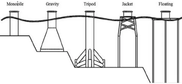
Horizontal-axis wind turbines are usually used for both on- and offshore wind turbines. However, in regards to environmental changes, Higgins and Foley (2013) describes that the foundation for offshore wind varies with the sea depth. There exist five different types of foundations that are visualized in Figure 3. Meanwhile, according to Tong (2010) the foundation for onshore site would consist of a concrete circular raft type or tubular tower. For offshore, Higgins and Foley (2013) highlights that the monopile foundation is suitable for depths of 0 - 30 m, whereas gravity based foundation can be applied for 0 - 40 m. Both tripod and jacket foundations can reach depths of 0 - 50 m, while floating can reach depths greater than 60 m.

Figure 3 Offshore Wind Turbine Foundation Types (Higgins & Foley, 2013)

3.2 Offshore Power Transmission for Wind Farms

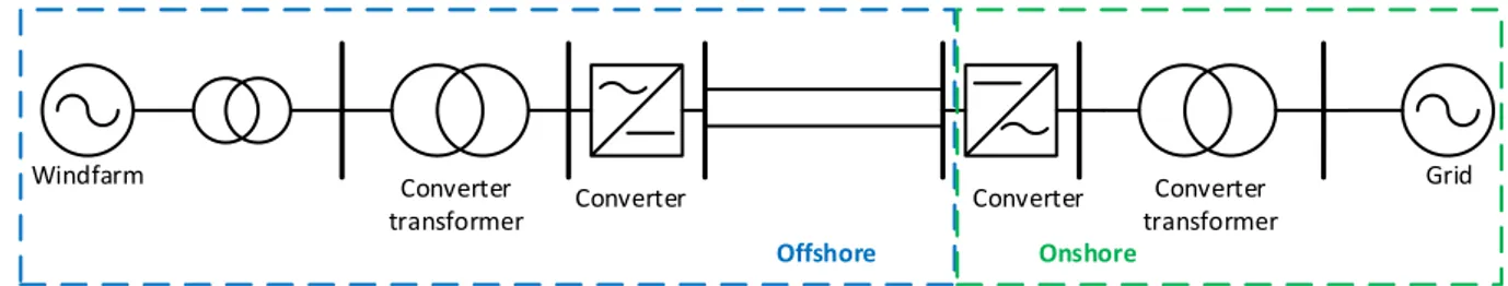
Offshore wind farms today use a collection grid within the farm which is then carried over to a transmission system to deliver power to the mainland. Each wind turbine in the farm has a transformer, usually placed at its base, to increase voltage levels from 690 V to a medium high voltage of 25 – 40 kV. Medium-voltage submarine power cables are typically buried around one meter in the seabed, they connect the wind turbines to an offshore substation. This is where the transmission system begins. The substation steps up voltage levels to between 130 - 170 kV to allow for less power losses and the use of submarine cables with smaller diameters which decreases the cost of the cable that is to be used for the long stretch to the mainland(Green, Bowen, Fingersh, & Wan, 2007). The newest energy transmission technology used in today’s offshore wind projects is High Voltage Direct Current – Voltage Source Conververs (HVDC-VSC).

HVDC using voltage-source converters is a relatively new technology with the first system installed 1997 in Hellsjön by ABB.de Alegría, Martín, Kortabarria, Andreu, and Ereño (2009) explains that HVDC-VSC uses high power Insulated-Gate Bipolar Transistors (IGBTs) as switches rather than thyristors, this produces almost non-existent amounts of harmonic distortions which removes the need for large filters. A more compact converter station can then be made and therefore a smaller offshore platform can be used, which will lower costs. Although, it does come with higher power losses of around 4 – 5 %. A VSC system can also do a ‘black start’ which means that it can start from a dead grid. No start-up mechanism is therefore required for the offshore station, as well as the ability to start by itself even if the grid onshore has collapsed. A general schematic of a HVDC-VSC transmission system for offshore wind farm is shown in Figure 4.

Grid Converter Windfarm Converter Converter transformer Converter transformer Offshore Onshore

Figure 4 Offshore Wind Farm HVDC-VSC Transmission System

Korompili, Wu, and Zhao (2016) highlight another advantage with VSC technology, the ability to control both active and reactive power. Active power control provides the system with the capability to quickly level out dips in power generation, it can reduce the amount of active power injected to the grid or even consume active power if necessary. This means that the grid frequency can be regulated, which might prove very helpful in a situation where the onshore grid is weak. Reactive power control is used to sustain grid AC voltage levels, the converters can achieve this by adjusting its reactive current. Voltage support to the network is therefore another advantage of a VSC system.

These advantages with VSCs provides a number of benefits in terms of design and operation of wind turbines according to Korompili et al. (2016). By being able to decouple the wind farm from the grid, it can refrain from being grid code compliant which allows more focus on cost reduction efforts for the wind farm in terms of efficiency, reliability and standardization to be made.

3.3 Vanadium Redox Flow Batteries

Li et al. (2011) explains that battery technologies used today come with some serious limitations, specifically charging time and life cycle. Redox Flow Batteries (RFBs) are being developed to address these drawbacks. RFBs uses two electrodes and two different

circulating electrolyte solutions, a positive and a negative, in order to convert and store electrical energy in the form of chemical energy and then convert that stored energy back into electrical energy. The two solutions are separated by a membrane that keeps the solutions separate but still allows for ionic transport.

Figure 5 depicts the process for a vanadium redox flow battery (VRFB), the most commonly used type of RFB in todays’ industry. Zimmerman (2014) explains that this is where the reduction and oxidation between the different redox states occurs. While charging, Vanadium ion V3+ _{is reduced to V}2+ _{in the negative electrolyte and V}4+ _{is oxidized to V}5+ _{in the positive}

electrolyte. Discharging the battery is the reverse of this process. The supporting electrolyte is typically sulphuric acid, H2SO4,which is added to provide the right amount of solubility for

Figure 5 Vanadium Redox Flow Battery Schematic

Vanadium makes for a fitting electrolyte material since it has the same metal ions for both electrolyte solutions, preventing cell capacity deterioration as well as the fact that it can exist in multiple oxidation states (Zimmerman, 2014).

There are several advantages with RFBs over conventional batteries. These include indefinite life cycle, very low self-discharge, fast response time and high energy efficiency. The most valuable property is the ability to independently scale power generation and storage capacity. This is possible since the battery cell and electrolyte are separated. Furthermore, it allows electrical storage capacity to be increased by adding larger electrolyte tanks while power generation capacity can be increased by stacking battery cells together. The scalability of RFBs is therefore one of the most attractive aspects for industrial and network applications (Li et al., 2011).

According to Zimmerman (2014) the main disadvantage with VRFBs is currently the

relatively low energy density of 50 Wh/kg electrolyte compared to Lithium-ion batteries for instance, which can achieve an energy density of up to 250 Wh/kg. The current price of vanadium is also of concern with market prices of $35/kg2 _{being recorded on January 31}st _of

2018 (InvestmentMine, 2018). However, this is predicted to decrease drastically as new procurement methods for vanadium are developed and when demand for the metal increases.

3.4 Wind Farm and HVDC Transmission Costs

A report from Cavazzi and Dutton (2016) demonstrate a methodology for calculations of offshore wind farm costs, including HVDC-VSC system costs. Another report by Gonzalez-Rodriguez (2017)also shows other various methods to approximate certain component costs for wind turbine farms, one of these methods are described later in the bisections of Wind Farm and HVDC Transmission Costs.

The report by Cavazzi and Dutton (2016) described a general formula for calculating the total cost of producing electrical energy for a wind farm, namely: levelized cost of energy (LCOE). This provides a general economical comparison of different systems. The LCOE can be defined as:

LCOE =(CAPEX ∙ FCR) + OPEX E𝑎𝑛𝑛𝑢𝑎𝑙

[€/MWh] (1)

Where;

LCOE = levelized cost of energy [€/MWh] CAPEX = Initial Capital Cost [€]

OPEX = Annual Operation and Maintenance Cost [€] FCR = Annual Fixed Charge Rate [%]

Eannual = Annual Energy Production (electrical energy) [MWh]

The LCOE is described similarly with the same methodology as in Purvins et al. (2018), with the exception of different variable naming’s and operations and maintenance cost, fuel cost and carbon price are added to the equation.

For the LCOE calculation, following sections define detailed explanations for the CAPEX, OPEX, FCR and Eannual.

It should be noted that the naming of the variables in all equations have been modified and currency units from Pounds £ to Euros € have been adapted from the original to fit the context of the literature study as a whole.

According to the report by Cavazzi and Dutton (2016), the capital expenditures can be

summarized as the investment costs to be made in order for a wind turbine to be operational. The costs are divided into several categories as; Development and Consent, Turbine, Balance of Plant and Installation, and Commissioning. These categories can be further

sub-categorized, which are shown in the table under Appendix 1. The table also shows some estimated values for CAPEX, which can be used as a reference for a typical case. Cavazzi and Dutton (2016) stated that calculations for CAPEX could be defined as;

𝐶𝐴𝑃𝐸𝑋 =𝑐𝑡𝑢𝑟𝑏𝑖𝑛𝑒𝑠+𝑐𝑡𝑟𝑎𝑛𝑠𝑚𝑖𝑠𝑠𝑖𝑜𝑛_(1−𝑓+𝑐𝑓𝑜𝑢𝑛𝑑𝑎𝑡𝑖𝑜𝑛+𝑐𝑖𝑛𝑠𝑡𝑎𝑙𝑙+𝑐𝑐𝑜𝑛𝑠𝑒𝑛𝑡 𝑑𝑒𝑣.) (2) Where; 𝑐𝑡𝑢𝑟𝑏𝑖𝑛𝑒𝑠 = cost of turbines [€] 𝑐𝑡𝑟𝑎𝑛𝑠𝑚𝑖𝑠𝑠𝑖𝑜𝑛 = transmission cost [€] 𝑐𝑓𝑜𝑢𝑛𝑑𝑎𝑡𝑖𝑜𝑛 = cost of foundation [€] 𝑐𝑖𝑛𝑠𝑡𝑎𝑙𝑙 = cost of installation [€] 𝑐𝑐𝑜𝑛𝑠𝑒𝑛𝑡 = cost of consent [€]

𝑓𝑑𝑒𝑣. = development factor [%] (takes account for development, consent and overall

management, typically 5 %)

The individual costs for the CAPEX are described within sections 3.4.1.1-3.4.1.5. For these calculations the assumptions defined in section 3.4.1.6 are applicable.

Cost of Turbines:

For the cost of turbines, it was possible to approximate to a relevant value with basis from other real values. The following equation gave a regression to a set of data from different studies described in the report by Gonzalez-Rodriguez (2017) to evaluate an estimated cost of the wind turbines used in a wind farm.

𝑐𝑡𝑢𝑟𝑏𝑖𝑛𝑒𝑠= 1081 ∙ 𝐶𝐴𝑃𝑤𝑖𝑛𝑑−𝑓𝑎𝑟𝑚0,9984 (3)

Where;

𝑐𝑡𝑢𝑟𝑏𝑖𝑛𝑒𝑠 = the total cost of all turbines within a wind farm [k€2016]

𝐶𝐴𝑃𝑤𝑖𝑛𝑑−𝑓𝑎𝑟𝑚 = the overall capacity of the wind farm [MW]

If equation (3) is divided with the constant, 𝐶𝐴𝑃_{𝑤𝑖𝑛𝑑−𝑓𝑎𝑟𝑚}, it is possible to describe the cost as a CAPEX cost directly, which has the unit [𝑘€2016/MW]. Here, it is also important to note

that the euros are converted to their value in 2016.

In the other report written by Cavazzi and Dutton (2016), the cost of wind turbines were estimated to be: 1.5 M£/MW3_{. Additionally, if the floating technology is used, the CAPEX will}

be 50 % more expensive.

Cost of Foundation:

The CAPEX for foundation can be described as shown in equation (4). The estimation for this cost has basis on a polynomial regression for three different offshore foundation

technologies; Monopile, Jacket and Floating. The observed data for the regression is previous

data from real project costs for foundations. It should also be noted that the cost of steel determines the foundation cost as a function of water depth(Cavazzi & Dutton, 2016).

𝑐𝑓𝑜𝑢𝑛𝑑𝑎𝑡𝑖𝑜𝑛= 𝐶𝐴𝑃𝐸𝑋𝑓𝑜𝑢𝑛𝑑𝑎𝑡𝑖𝑜𝑛∙ 𝐶𝐴𝑃𝑤𝑖𝑛𝑑−𝑓𝑎𝑟𝑚=

= ((𝑎𝑥2+ 𝑏𝑥 + 𝑐) + ([𝑑𝑎𝑦𝑠]𝑖𝑛𝑠𝑡𝑎𝑙𝑙 + [𝑑𝑎𝑦𝑠]𝑡𝑜−𝑠𝑖𝑡𝑒) ∙ 𝑐𝑗𝑎𝑐𝑘−𝑢𝑝)

∙ 𝐶𝐴𝑃𝑤𝑖𝑛𝑑−𝑓𝑎𝑟𝑚

(4)

Where;

𝐶𝐴𝑃𝐸𝑋𝑓𝑜𝑢𝑛𝑑𝑎𝑡𝑖𝑜𝑛 = The Cost of a foundation [€/MW]

𝑐𝑗𝑎𝑐𝑘−𝑢𝑝 = The Cost of foundation installation vessel [M€/day]

x = Water depth [m]

a, b, c = Constant values (see Table 1)

[𝑑𝑎𝑦𝑠]𝑖𝑛𝑠𝑡𝑎𝑙𝑙 = Number of days to install (see Table 1)

[𝑑𝑎𝑦𝑠]_{𝑡𝑜−𝑠𝑖𝑡𝑒} is the journey time in days, see equation (5).

[𝑑𝑎𝑦𝑠]_{𝑡𝑜−𝑠𝑖𝑡𝑒} =

2 ∙ 𝑐𝑗𝑎𝑐𝑘−𝑢𝑝∙ (𝑑₁₀₀₀₎𝑛𝑒𝑎𝑟

(𝑣𝑗𝑎𝑐𝑘−𝑢𝑝∙ [ℎ𝑜𝑢𝑟𝑠]𝑤𝑜𝑟𝑘𝑖𝑛𝑔−𝑑𝑎𝑦∙ [𝑛]𝑝𝑒𝑟−𝑣𝑖𝑠𝑖𝑡)

(5) Where;

𝑑𝑛𝑒𝑎𝑟 = The Distance to the nearest deep water port [m]

𝑣𝑗𝑎𝑐𝑘−𝑢𝑝 = The Speed of the installation vessel [km/h]

[ℎ𝑜𝑢𝑟𝑠]_{𝑤𝑜𝑟𝑘𝑖𝑛𝑔−𝑑𝑎𝑦} = Length of working day [h]

[𝑛]_{𝑝𝑒𝑟−𝑣𝑖𝑠𝑖𝑡} = The Number of foundation pieces that can be carried per trip

Furthermore, additional manufacturing costs of 50 % and 20 % of the total 𝐶𝐴𝑃𝐸𝑋𝑓𝑜𝑢𝑛𝑑𝑎𝑡𝑖𝑜𝑛

are added for jacket and floating respectively according to Cavazzi and Dutton (2016).

Cost of Installation:

The CAPEX for installation summarizes the costs of shipping turbines to their respective installation sites, installation of the turbines and the cabling in-between. The equation for this estimation is described as following (Cavazzi & Dutton, 2016):

𝑐𝑖𝑛𝑠𝑡𝑎𝑙𝑙 = 𝐶𝐴𝑃𝐸𝑋𝑖𝑛𝑠𝑡𝑎𝑙𝑙∙ 𝐶𝐴𝑃𝑤𝑖𝑛𝑑−𝑓𝑎𝑟𝑚=

= ([𝑑𝑎𝑦𝑠]𝑖𝑛𝑠𝑡𝑎𝑙𝑙 + [𝑑𝑎𝑦𝑠]𝑡𝑜−𝑠𝑖𝑡𝑒) ∙ 𝑐𝑗𝑎𝑐𝑘−𝑢𝑝

+ (𝑐𝑐𝑎𝑏𝑙𝑖𝑛𝑔 + 𝑐𝑐𝑎𝑏𝑙𝑒,𝑖𝑛𝑠𝑡𝑎𝑙𝑙) ∙ 𝑙𝑐𝑎𝑏𝑙𝑖𝑛𝑔

[𝑑𝑎𝑦𝑠]_{𝑡𝑜−𝑠𝑖𝑡𝑒} = The journey time in days, see equation (5). Note that [𝑛]𝑝𝑒𝑟−𝑣𝑖𝑠𝑖𝑡 becomes the

number of turbines that can be carried per trip 𝑐𝑐𝑎𝑏𝑙𝑖𝑛𝑔 = Intra-array cable cost [M€/km]

𝑐𝑐𝑎𝑏𝑙𝑒,𝑖𝑛𝑠𝑡𝑎𝑙𝑙 = Intra-array cable installation cost [M€/km]

𝑙𝑐𝑎𝑏𝑙𝑖𝑛𝑔 = Length of the Intra-array cable [km]

Cost of Connection:

The CAPEX cost for connection of the wind farm to an electrical grid is described in equation (7) from the report by Cavazzi and Dutton (2016).

𝑐𝑡𝑟𝑎𝑛𝑠𝑚𝑖𝑠𝑠𝑖𝑜𝑛= 𝐶𝐴𝑃𝐸𝑋𝑡𝑟𝑎𝑛𝑠𝑚𝑖𝑠𝑠𝑖𝑜𝑛∙ 𝐶𝐴𝑃𝑤𝑖𝑛𝑑−𝑓𝑎𝑟𝑚= = [( 𝑑 1000) ∙ 𝑛 ∙ 𝑐]𝑐𝑎𝑏𝑙𝑒 + [𝑛 ∙ 𝑐]𝑜𝑓𝑓𝑠ℎ𝑜𝑟𝑒+ [𝑛 ∙ 𝑐]𝑜𝑛𝑠ℎ𝑜𝑟𝑒 (7) Where; 𝐶𝐴𝑃𝐸𝑋𝑡𝑟𝑎𝑛𝑠𝑚𝑖𝑠𝑠𝑖𝑜𝑛 = Transmission cost [€/MW]

𝑑𝑐𝑎𝑏𝑙𝑒 = Cable distance between off- and onshore substation [m]

[𝑛]_{𝑐𝑎𝑏𝑙𝑒} = Number of cables to shore 𝑐𝑐𝑎𝑏𝑙𝑒 = Cable cost [M€/km]

[𝑛]_{𝑜𝑓𝑓𝑠ℎ𝑜𝑟𝑒} = Number of offshore platforms 𝑐𝑜𝑓𝑓𝑠ℎ𝑜𝑟𝑒 = Cost per platform [M€]

[𝑛]𝑜𝑛𝑠ℎ𝑜𝑟𝑒 = Number of onshore convertor stations

𝑐𝑜𝑛𝑠ℎ𝑜𝑟𝑒 = Cost per onshore convertor station [M€]

Another report by Xiang, Merlin, and Green (2016) estimates the costs for a HVDC system in the same manner, but with a slightly more recent empirical formulas for convertor station and platform costs.

Cost of Consent

The cost of consent according to Cavazzi and Dutton (2016) summarizes the costs for environmental survey, seabed survey, met mast and development services. The costs are shown in the table located in Appendix 1.

Assumptions

The assumptions relevant for the CAPEX of turbines, foundations, connections and installations are shown below in table format, these assumptions are from the report by Cavazzi and Dutton (2016). However, the values have been converted from (£, GBP) to (€, EUR) according to the values in Appendix 3.

Table 1 Cost of Foundations Parameters

a b c [𝑑𝑎𝑦𝑠]𝑖𝑛𝑠𝑡𝑎𝑙𝑙

Monopile 0.0011 0.0023 1.2253 1

Jacket 0.0008 -0.0154 1.5847 3

Floating 0 0.0017 3.732 2

Number of turbines per visit [𝑛]_{𝑝𝑒𝑟−𝑣𝑖𝑠𝑖𝑡} 5

Speed of installation vessel [km/h] 𝑣𝑗𝑎𝑐𝑘−𝑢𝑝 20

Length of the working day [h] [ℎ𝑜𝑢𝑟𝑠]_{𝑤𝑜𝑟𝑘𝑖𝑛𝑔−𝑑𝑎𝑦} 24

Material cost of steel [€/tonne] 𝑐𝑠𝑡𝑒𝑒𝑙 2167.2

Cost of foundation installation vessel [M€/day] 𝑐𝑗𝑎𝑐𝑘−𝑢𝑝 0.1805445

Table 2 Cost of Connection Parameters

Number of offshore platforms [𝑛]𝑜𝑓𝑓𝑠ℎ𝑜𝑟𝑒 2

Cost per platform [M€] 𝑐𝑜𝑓𝑓𝑠ℎ𝑜𝑟𝑒 132.3993

Number of cables to shore [𝑛]𝑐𝑎𝑏𝑙𝑒 2

Cable cost [M€/km] 𝑐𝑐𝑎𝑏𝑙𝑒 1.083267

Number of onshore convertor stations [𝑛]𝑜𝑛𝑠ℎ𝑜𝑟𝑒 2

Cost per onshore convertor station [M€] 𝑐𝑜𝑓𝑓𝑠ℎ𝑜𝑟𝑒 78.23595

Table 3 Cost of Installation Parameters

Number of days on site to install each turbine [𝑑𝑎𝑦𝑠]_{𝑖𝑛𝑠𝑡𝑎𝑙𝑙} 2 Length (intra-array) cable [km] 𝑙𝑐𝑎𝑏𝑙𝑖𝑛𝑔 350

Intra-array cable cost [M€/km] 𝑐𝑐𝑎𝑏𝑙𝑖𝑛𝑔 0.1805445

Intra-array cable installation cost [M€/km] 𝑐𝑐𝑎𝑏𝑙𝑒,𝑖𝑛𝑠𝑡𝑎𝑙𝑙 0.120363

Number of turbines per visit [𝑛]𝑝𝑒𝑟−𝑣𝑖𝑠𝑖𝑡 5

Speed of installation vessel [km/h] 𝑣𝑗𝑎𝑐𝑘−𝑢𝑝 20

Length of the working day [h] [ℎ𝑜𝑢𝑟𝑠]𝑤𝑜𝑟𝑘𝑖𝑛𝑔−𝑑𝑎𝑦 24

The Eannual summarizes the annual electrical energy production of a wind farm. A general

approach is described by Lakshmanan, Liang, and Jenkins (2015); the first step is to calculate the Weibull probability distribution as described:

𝑓(𝑣𝑤) = 𝑘 𝑐∙ ( 𝑣𝑤 𝑐) 𝑘−1 ∙ 𝑒(−( 𝑣𝑤 𝑐) 𝑘 ) ₍₈₎ Where;

𝑣𝑤 = The Wind speed [m/s]

𝑓(𝑣𝑤) = The Weibull probability distribution function of occurrence of wind speed 𝑣𝑤

k = Shape parameter c = Scale parameter

The Weibull probability distribution is a function that specifies the occurrence of wind speed and its probability.

The second step is to calculate the power generated, as shown below: 𝑃𝑔𝑒𝑛,𝑊𝑇(𝑣𝑤) =

1

2∙ 𝜌 ∙ 𝐴 ∙ 𝐶𝑝∙ 𝑣𝑤

3 ₍₉₎

Where;

𝑃𝑔𝑒𝑛,𝑊𝑇(𝑣𝑤) = Power generated at each wind speed [W]

𝜌 = Air density [kg/m3_]

𝐴 = Area covered by the turbine blades [m2_] 𝐶𝑝 = Power coefficient

The power coefficient describes the wind turbine characteristics and decides how efficiently the conversion of wind energy can be turned into electrical energy. This principle follows Betz law, whereas it is stated that power coefficient cannot exceed values greater than 59.3 %. (Wizelius, 2015)

For the final step, using the equations (8) and (9), electrical energy production is received accordingly to:

𝐸𝑎𝑛𝑛𝑢𝑎𝑙 = [𝑛]𝑊𝑇∫ ((𝑃𝑔𝑒𝑛,𝑊𝑇(𝑣𝑤)) ∙ 𝑓(𝑣𝑤) ∙ 8760) 𝑑𝑣𝑤 𝑣𝑚𝑎𝑥

𝑣_𝑚𝑖𝑛 (10)

Where;

𝐸𝑎𝑛𝑛𝑢𝑎𝑙 = Annual energy production [MWh]

[𝑛]_𝑊𝑇 = Number of wind turbines 𝑣𝑚𝑎𝑥 = Cut out wind speed [m/s]

The OPEX is described by Cavazzi and Dutton (2016)as: 𝑂𝑃𝐸𝑋 = 𝑐𝑓𝑖𝑥𝑒𝑑+ 𝑐𝑓𝑒𝑒+ (( 𝑑𝑛𝑒𝑎𝑟,𝑝𝑜𝑟𝑡 1000 ) ∙ 𝑐𝑣𝑎𝑟 100) (11) Where; 𝑐𝑓𝑖𝑥𝑒𝑑 = Fixed cost [€/MWh]

𝑐𝑓𝑒𝑒 = Cost for port fee [€/MWh]

𝑑𝑛𝑒𝑎𝑟,𝑝𝑜𝑟𝑡 = Distance to the nearest port [m]

𝑐𝑣𝑎𝑟 = Variable costs [€/MWh]

For the OPEX calculation following assumptions are possible according to Cavazzi and Dutton (2016),where the euro conversion was adapted.

Table 4 OPEX Parameters

Fixed costs [€/MWh] 𝑐𝑓𝑖𝑥𝑒𝑑 21.66534

Variable costs [€/100 km] 𝑐𝑣𝑎𝑟 7.22178

Port fees [€/MWh] 𝑐𝑓𝑒𝑒 3.61089

According to Purvins et al. (2018) the capital recovery factor CRF which is equivalent to FCR can be calculated as following:

𝐹𝐶𝑅 = 𝐶𝑅𝐹 = 𝑟 ∙ (1 + 𝑟)

𝑛

(1 + 𝑟)𝑛_{− 1} (12)

Where;

r = Interest rate

n = Operational life [years]

The overall system losses consider the collection losses and the transmission losses. The collection losses include three main categories according to the report Lakshmanan et al. (2015), namely; power electronics losses, collection cables losses and the losses in collection system components.

𝐸𝑙𝑜𝑠𝑠𝑒𝑠,𝐴𝐶 = ∫ (𝑃𝑃𝐸,𝐴𝐶(𝑣𝑤) + 𝑃𝑐𝑎𝑏𝑙𝑒,𝐴𝐶(𝑣𝑤)) ∙ 𝑓(𝑣𝑤) ∙ 8760 ∙ 𝑑 𝑣_𝑚𝑎𝑥

𝑣𝑚𝑖𝑛

𝑣𝑤 (13)

Where;

𝐸𝑙𝑜𝑠𝑠𝑒𝑠,𝐴𝐶 = Annual energy losses [MWh]

𝑣𝑚𝑎𝑥 = Cut out wind speed [m/s]

𝑣𝑚𝑖𝑛 = Cut in wind speed [m/s]

𝑃𝑃𝐸,𝐴𝐶 = Total power electronic losses [MW]

𝑃𝑐𝑎𝑏𝑙𝑒,𝐴𝐶 = Total cable losses [MW]

The power electronics includes components such as converters (AC-DC, DC-AC and DC-DC) and transformers. According to Glover, Overbye, and Sarma (2017), cable losses in the AC-collection context are mainly related to series resistance R and shunt conductance G. The cable losses can be acknowledged as power losses, defined with I2_{R and V}2_{G losses. I}2_{R losses}

occur when current is applied to the transmission line and there is resistance within the line, which results in ohmic losses. Meanwhile, V2_{G losses occur when voltage is applied to the}

line, which causes insulator leakages and dielectric losses. During normal operation

conditions the I2_{R losses are greater than V}2_{G losses. In DC-transmission context the losses}

mainly consist of I2_{R losses.}

Transmission Line Losses VSC-HVDC

To determine the overall losses for the transmission between the onshore and offshore substations, the method from Negra, Todorovic, and Ackermann (2006) can be used. The method includes the losses at the converter stations (on- and offshore) and the cabling between them.

For the offshore station, the power after the convertor station can be defined as:

𝑃1= (1 − 𝑥𝑠) ∙ 𝑃𝑖𝑛 (14)

Where;

𝑃1 = The offshore convertor station power [W]

𝑥𝑠 = The convertor station loss [%]

𝑃𝑖𝑛 = The power before convertor station [W]

The cable power losses can then be defined as:

𝑃𝐶 = 𝑃1− 𝑃2 = 𝑅 ∙ 𝐼2= 𝑅 ∙ ( 𝑃1 𝑉𝐶 ) 2 (15) Where;

𝑃𝐶 = The cable power losses [W]

𝑅 = The cable resistance [Ω]

𝐼 = The current flowing in the cable [A] 𝑉𝐶 = The rated voltage of the cable [V]

At the onshore station, the outlet power becomes:

𝑃𝑜𝑢𝑡= (1 − 𝑥𝑠) ∙ 𝑃2 (16)

Where;

𝑃𝑜𝑢𝑡 = The power after the convertor station [W]

In this method, Negra et al. (2006) states that 𝑥𝑠 remains constant for both on- and offshore

convertor stations. By using the already estimated value of 1.24 % for platform converter losses, the value for convertor station loss is then 𝑥_𝑠= 0.0124.

For the transmission line between onshore and offshore substations, the ohmic losses can be calculated by taking DC-resistance, RDC and multiply it with the transmitted current to

receive the total power loss for the transmission line. The DC-resistance can be calculated by using the following equation and data from Glover et al. (2017):

𝑅𝐷𝐶 =

𝜌𝑇∙ 𝑙

𝐴 (17)

Where;

𝑅𝐷𝐶 = The DC-resistance of conductor [Ω]

𝜌𝑇 = Conductor resistivity at temperature T [Ωm]

𝑙 = Conductor length [m]

𝐴 = Conductor cross-sectional area [m2]

For determining the conductor area of the cable required, relevant cable data can be used, which is found in datasheets from the manufacturers.

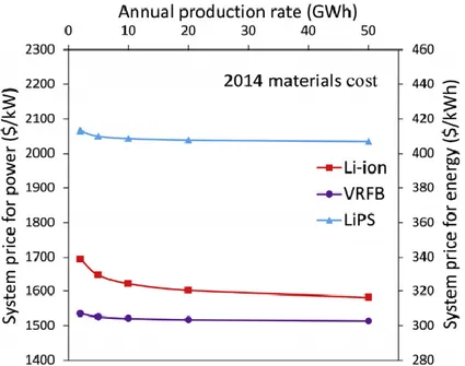
3.5 VRFB System Costs

A study conducted by Ha and Gallagher (2015) titled Estimating the system price of redox flow batteries for grid storage, present a comprehensive Unit Price Less Materials (UPLM) analysis of VRFB systems. UPLM include plant investment costs and unit costs for the battery packs. The unit costs consist of variable costs such as direct labour, warranty as well as research and development. However, the study by Ha and Gallagher (2015) also includes an analysis of the total system cost of VRFBs for both present material costs and predicted future costs. Projections for Li-ion battery systems and Lithium Polysulfide semi-flow

increase in the near future. The baseline used in the study are an annual production rate of 100,000 battery stacks with a continuous stack power of 20 kW and an energy storage of 100 kWh. If higher power ratings are required, the stacks can be combined in parallel or series to provide a suitable value.

Projections for the entire battery system prices are also presented in the study, which include projections for 2014 material costs as well as predicted future material costs. These are shown in Figure 6 and Figure 7 respectively. Both figures show VRFBs as being the least expensive option for energy storage systems.

Figure 6 System price as a function of annual production rate using 2014 material costs (Ha & Gallagher, 2015)

Figure 7 System price as a function of annual production rate using future state material costs (Ha & Gallagher, 2015)

There is however uncertainty in these results, with Ha and Gallagher (2015) stating a system price variation of ± 28 % for 95 % confidence intervals for VRFB systems. This large disparity is mostly due to the large variation in vanadium commodity price on the market. They further state that the costs for the carbon felt and ion-exchange membrane for flow batteries are key obstacles for broader deployment. While VRFBs have benefited greatly from efforts made in fuel cell development, there is still a long way to go before they can reach the same amount of production rate as Li-ion. One thing not taken into consideration in this paper is site

installation cost though, which typically is a large factor in system capital cost. This cost is highly location specific and is therefore difficult to estimate.

In conclusion Ha and Gallagher (2015) describe flow batteries as being able to utilize the advantages of production volume at much lower rates than Li-ion and suggest that just moderate levels of production (e.g. 20,000 20-kW batteries per year) could lead to cost-effective deployment of flow batteries for energy storage applications.

Another, more recent study, conducted by Minke, Kunz, and Turek (2017) describes another techno-economic model for determining VRFB system costs. Component and electrochemical models were used to calculate current cost of equipment such as the stacks and electrolyte, as well as identifying specific cost reduction potentials for each part of the system.

Minke et al. (2017) derive a linear cost function (see equation (18)) from the model results in order to determine system costs for varying VRFB systems. The results provided cost rates for both the power subsystem and the energy subsystem of the VRFB, with cpower = 1080 €/kW and cenergy = 385 €/kWh. The function is stated to provide accurate results within the scope of P = 1 MW – 20 MW and E/P = 4 h or 8 h.

𝐶𝑠𝑦𝑠𝑡𝑒𝑚 = 𝑃 ∙ 1080 [ € 𝑘𝑊] + 𝐸 ∙ 385 [ € 𝑘𝑊ℎ] (18) Where;

Csystem = Total system cost P = Cell stack power

E = Energy storage capacity

Transferring the electrolyte from one place to another requires transportation. In this degree work the transportation occurs at sea meaning that tankers are required to transfer and hold the electrolyte from an offshore wind farm to an onshore station. This brings costs along with it.

In order to transport and hold the electrolyte, a chemical tanker is needed. Wärtsilä (2018) describes a chemical tanker as being a cargo ship specifically constructed and used to carry

short sea travels typically range from 10,000 to 35,000 dwt according to a market review by UNCTAD (2017).

A market review given by Finance (2016) provide information on time charter rates for chemical tankers, which in November 2016 were on average 16,000 $/day. This value does however fluctuate quite heavily from year to year, which make it a highly uncertain value. Newly built chemical tankers are stated to be priced at 33 M$ while second-hand values of the ships go down with age, from 22 M$ for a 5-year-old ship to 10 M$ for a 15-year-old ship, the price does depend heavily on the carrying capacity of the ships however.

A report from Turker, Arroyo Klein, Hammer, Lenz, and Komsiyska (2013) titled “Modeling a vanadium redox flow battery system for large scale applications” explores the various losses in a VRFB unit, both for charging and discharging operations. These energy losses occur in the stacks during the electrochemical conversion as well as auxiliary power consumption of the surrounding systems drawing some energy, such as the hydraulic circuits. Losses such as the power demand of the control system and the air conditioning system are neglected in these calculations since their minimal effect on a megawatt-size systems’ efficiency. The main losses in the system are coulombic losses, overvoltage losses and pumping losses, with inverter and rectifier losses depending on which connection the battery has, AC or DC. Figure 8from the report describes the process for both operational modes. Rectifier and inverter losses in their report were assumed to be 5 %.

The State of Charge (SOC) is one of the main factors that affect battery performance. Turker et al. (2013) evaluated efficiency at multiple levels of SOC in their study. The efficiency stayed relatively stable during the discharge process, the efficiency dropped about 15 % when SOC reached above 75 % during the charge process. This happened because pumping power demand increases significantly at high SOC levels. Most of the time the efficiency stays stable, with the round-trip efficiency holding at around 64 % between 20 – 75 %. The full efficiency results are shown in Figure 9.

4 DESCRIPTION OF ACTUAL STUDY

The description of actual study reviews the scenario laid out for each transmission system as well as which calculation methods and assumptions that has been applied to retrieve the results.

4.1 Wind Farm Scenario

The wind farm scenario was initially created by choosing the appropriate components to be used. These were then applied within a layout, and a location for the farm was defined. The location included appropriate wind data for the wind farm.

The components that were chosen for the scenario depended on the transmission system. Therefore, a general model for the wind farm was created that could be applied for each transmission method.

Wind Farm

The wind farm consisted of wind turbine model; V112-3 MW, manufactured by Vestas (2018). The summarized data for the model is shown in Appendix 2.

The same model of wind turbine was used for the whole wind farm and the amount of wind turbines was set to 20, which would result in a total rated power of 60 MW for the entire wind farm. This is quite a low sized wind farm compared to real scenarios. The size was decided upon since a VRFB system of the magnitude of 500 MW with today’s energy densities and cell voltages would require such impossibly large cell stacks and electrolyte tanks. Therefore, a comparison between the two methods would be redundant.

The layout for the wind farm is visualized in Figure 10. Here, the wind turbines (WTs) consisted of a generator (AC power source) and a transformer. Four sets of five turbines in series were connected in parallel to a bus via an AC collection system. Each wind turbine was separated by a distance of 1 km from the other turbines, while the connections to the bus from the wind turbine series had a distance of 3 km respectively. The bus was connected to a linking point (LP) that could be connected to a HVDC- or a VRFB transmission system.

Figure 10 Wind Farm Layout

HVDC System

The HVDC system, as mentioned in the literature study (section 3.2.1); consisted of an offshore substation, a submarine cable and an onshore substation. The overall system can be seen in Figure 11. The offshore substation was connected to the wind farm (note linking point, LP). The substation consisted of two AC to DC converters and transformers. Submarine cabling, consisting of two lines, were connected between the off- and onshore substations. The distance between these stations are indicated with a variable; dcable. The

onshore substation consisted of similar components as the offshore substation. The difference was that onshore substation has DC to AC converters and the transformers has different voltage ratings.

dcable

LP

Onshore

substation

Offshore

substation

Grid

Figure 11 HVDC System Layout

VRFB System

The overall design of the VRFB system did not differ much from the HVDC system. The main difference was that the VRFB system used a transportation vessel instead of a submarine cable to transfer energy. This method is done via charging and discharging the VRFB at

for discharging and afterwards transmit the energy from electrolyte to the grid. An energy density of 50 Wh/kg was assumed for this degree work.

The discharge time at the onshore station would become a problem with using VRFBs. Since the vessel is discharging, nothing is charging at the offshore station. This means that at least two tanker vessels have to be used in rotation. In that way one vessel can charge at the offshore station while the other discharges at the onshore station, the size and number of ships in use depended on what discharge time that was chosen. Figure 12 shows a general layout of the system.

d

The size and number of cell stacks and electrolyte tanks was determined depending on the power and energy output of the wind farm as well as what the number of ships and their respective discharge time would be. The model suggested by Minke et al. (2017) was used to determine the power and number of cells for each cell stack required for the proposed wind farm. Cell voltage is dependent on SOC, in this case the value was averaged for a SOC of 20 – 80 % as to keep efficiency as high and consistent as possible.

Since the cell stacks would have to reach the same 60 MW that the wind farm could

potentially put out, 3 of the 20 MW power subsystems mentioned by Minke et al. (2017) was used. This model used 250 kW stacks with 75 cells in each which would result in a stack area of 201 m2_{. To charge each stack with 250 kW of power a voltage of 980 V and a current of 252}

A can be used, in accordance with a VRFB project at Fraunhofer-Gesselschaft, Germany, which uses similar stacks (Alotto, Guarnieri, & Moro, 2014). For one 20 MW system a total of 80 stacks would be required, these can be placed on top of each other to keep platform area down at the offshore station. The set-up of stacks at the discharging station onshore was assumed to be of equivalent size and numbers.

To compare different possible solutions for this transmission method in terms of CAPEX and OPEX, two different methods of electrolyte charging/discharging and transportation were compared. The first consisted of having two larger ships in rotation, each with a discharge time of 50 h. The other scenario had a chosen discharge time of 8 h, with four vessels used in rotation.

The location chosen for the wind farm was off the east coast of Great Britain, since they are currently expanding their offshore wind power dramatically and there is plenty of wind data in the area readily available. The wind speed data was gathered from the Marine Data Exchange database at a height of 82 m from the Greater Gabbard wind farm situated about 22.5 km off the coast, see Figure 13.

Figure 13 Location of Greater Gabbard Wind Farm (marked in light green) (Bing, 2018) The data was taken from both the northwest and southwest direction and was measured every ten minutes, in this degree work an average value between these two directions was used at each time interval for the years 2006 - 2009. The data was then separated into values for each month of the year using Excel, in order to determine energy output of the wind farm on a monthly basis.

4.2 Calculations

The following section describes the energy calculations that were made for the wind farm, including system losses for the two transmission systems.

Wind Farm Energy Output

The wind speed data collected and aggregated was imported into MATLAB where a Weibull distribution parameter function made by Roche (2013) was applied, which uses a graphical method encompassing line fitting to determine both shape- and scale parameters from said data. These parameters were then used in equation (8) to provide the Weibull distribution for every month.

The swept area of the turbine specified in Appendix 2 was applied to equation (9) with assumptions being an air density of 1.225 kg/m3_{. The power coefficient for different wind}

speeds was determined with the turbines’ power curve supplied by the manufacturer and through the use of equation (9). These two equations were combined in equation (10), integrating over the turbines’ cut-in- and cut-out speeds of 3 m/s and 25 m/s respectively to determine the total energy output each month. These were summed up to acquire an annual energy output for the wind farm.

Collection System Losses

The power electronic losses required for the use of equation (13) for the AC-collection system was estimated to (Lakshmanan et al., 2015):

• Full scale converter at each turbine (Si converters): 6.5 % • 50Hz transformer losses at each turbine: 1 %

The power output of the wind farm from previous calculations was used here to estimate the power electronic losses. The loss assumptions made above as well as the power output results were applied to equation (13). These losses also depend on the number of turbines used in the system, since the converters and step-up transformers are used at each turbine.

The collection cable system was assumed to be AC and with this the AC resistance of the cables was calculated with equation (19), (Nord, 2011).

𝑅𝐴𝐶 = 𝑅𝐷𝐶∙ (1 + 𝑦𝑠+ 𝑦𝑝) [

Ω

𝑘𝑚] (19)

The DC resistance was computed with equation (17) with the resistivity of copper at 90° Celsius being used, which lies at 21.5 Ωmm2_{/km. ys is the skin effect factor which was given}

𝑦𝑠 = 𝑥𝑠4 192 + 0.8𝑥𝑠4 (20) 𝑥𝑠2 = 8𝜋𝑓 𝑅𝐷𝐶 ∙ 10−7_{∙ 𝑘} 𝑠 (21)

The cables were presumed to be round which sets the coefficient ks to 1 and the frequency f was presumed to be 50 Hz. A proximity effect factor was also calculated since the cables used were decided to be three-core cables. This was done through equations (22) and (23).

𝑦𝑝= 𝑥𝑝4 192 + 0.8𝑥𝑝4 (𝑑𝑐 𝑠) 2 [ 0.312 (𝑑𝑐 𝑠) 2 + 1.18 𝑥𝑝4 192 + 𝑥𝑝4 + 0.27 ] (22) 𝑥𝑝2= 8𝜋𝑓 𝑅𝐷𝐶 ∙ 10−7∙ 𝑘𝑝 (23)

Where dc is the diameter of the conductor, s is the distance between conductor axes and kp is equal to 0.8 using the same presumptions as for ks.

The active losses of the cabling were then calculated with equation (24).

𝑃𝑙 = 𝐼2∙ 𝑅𝐴𝐶 = ( 𝑛𝑊𝑇∙ 𝑃𝑖 𝑈 ∙ cos(𝜑)) 2 ∙ 𝑅𝐴𝐶 [ 𝑊 𝑘𝑚] (24)

Where nWT is the number of wind turbines at each cable row, Pi the power at wind speed i, U the rated voltage and cos(𝜑) the power factor. This equation was integrated over each wind speed within the working range of the farm in order to acquire the total power loss from the cables. In this degree work the number of turbines per row was set to 5, with the rated voltage being set to 33 kV and an assumed power factor of 1 (reactive power compensation is

assumed). The total length of the cables across the entire system was 28 km with 4 rows in total.

Determination of cable was aided by calculating the maximum amount of current the cable would have to withstand within the system, this was done with equation (25).

𝐼𝑚𝑎𝑥=

𝑛𝑊𝑇∙ 𝑃𝑟𝑎𝑡𝑒𝑑

𝑈 ∙ cos(𝜑) [𝐴] (25)

A cable datasheet from ABB (2010) which included current ratings for various cables was used to determine an appropriate conductor area. In this case a three-core, copper cable with a conductor area of 400 mm2 _{and a diameter of 23.2 mm was chosen to provide a good safety}

margin.