Variations in the external cost of transport air pollution : The case of Sweden

Full text

(1)VTI notat 36A • 2003. VTI notat 36A-2003. Variations in the external cost of transport air pollution – the case of Sweden. Authors. Lena Nerhagen, VTI Håkan Johansson, TFK. Research Division Transport Economics Project number. 92055. Project name. Estimation of the Environmental Costs of the Transport Sector in Sweden with the ”ExternE-approach”. Sponsor. Vinnova.

(2) Contents. Page. Summary. 3. 1 1.1 1.2. Introduction Background The all-modes study. 5 5 6. 2 2.1 2.2 2.3. Variations of costs in the all-modes study Costs due to NO2 and SO2 for all transport modes Costs on urban roads The general assumptions and Swedish conditions. 8 9 11 15. 3 3.1 3.2 3.3. Cost estimates in other studies The ASEK-values The Marginal cost case studies in 2002 The BeTa-estimates. 17 17 20 21. 4 4.1 4.1.1 4.1.2 4.1.3 4.2. Generalizations of the cost estimates Situation specific determinants Emissions Dispersion modelling Effects and values Large or small emissions. 24 24 24 25 26 26. 5 5.1 5.2 5.3. Discussion Valuing the effects of transport air pollution Policy implications Further research. 27 27 29 30. References. 32. Appendix 1: Particle-emissions in the EU driving cycle for different vehicles. VTI notat 36A-2003.

(3) Summary In recent years large efforts have been devoted in EU-funded research projects, i.e. the ExternE-projects, to the development of an approach that can be used to estimate the external costs of air pollution. The calculation in these projects is based on the so called Impact pathway approach where the impacts from air pollution are assessed and valued. This approach has now been used to estimate the cost of air pollution of transport in Sweden for the year 2000. In addition, we have used abatement cost estimates to include the costs due to acidification and eutrophication. This is a joint project between VTI, TFK and IER at the University of Stuttgart. This report presents and discusses the results from this project, “the all-modes study”, regarding air pollutants with a local and regional dispersion. It also relates the results from this project to cost estimates in other studies. Cost estimates have been calculated for all transport modes. For road transport, estimates were calculated for extra urban and urban traffic and also for two cases, Skellefteå and Stockholm. The purpose was to obtain information on the variation in costs between different traffic situations. Such information is an input in the evaluation of infrastructure investments and is also a basis for marginal cost pricing. The costs vary since there is a large number of variables that influence the estimates. Costs will depend upon which pollutant we consider and where the emissions occur. Costs will also depend upon other relationships such as the number of people being asthmatics in a population and the value placed on an asthma attack. For the latter, the assumptions used in the all-modes study are the same as those used in the EU-funded UNITE-project. The first part of this report describes the results of the all-modes study. First the cost per tonne for NO2 and SO2 for all transport modes are compared. It is established that the estimates depend upon where in the country the emissions take place, north or south, countryside or urban area. The main reasons are differences in population density in the area where the emissions occur and also the geographical location within the country. For pollutants with a regional dispersion, the cost per tonne will also vary between different modes since these pollutants involve in chemical reactions on the regional scale. Thereafter we compare the average cost per km for different vehicles in urban areas in Sweden. For locally dispersed pollutants, costs are high for all diesel vehicles since they have high particle emissions. These costs are highest for bus and HDV. For regionally dispersed pollutants the total cost is again highest for bus and HDV and lowest for two-wheelers. The abatement cost estimates corresponds to around 50 % of the total cost. Comparing the average costs for all urban areas with the costs for Skellefteå and Stockholm, we find that the costs are lower in Skellefteå than in the other two cases, for separate pollutants and also in total. This is as expected since Skellefteå is located in the north of Sweden. In the second part of the report the results in the all-modes study have been compared to those in other studies. The first concerns the values that are presently used as external costs for transport air pollutants in Sweden, the ASEK-values. These latter values are higher, mainly due to differences in the assumptions regarding the dose that individuals are exposed to. The second comparison concerns the estimates from two marginal cost case studies, one for maritime transport and one for an airport. Their estimates for locally dispersed pollutants are lower than those in our all-modes study. A reason for this could be the level of. VTI notat 36A-2003. 3.

(4) detail in the local dispersion modeling. Finally, we have compared our estimates for particles and locally dispersed SO2 emissions with those recommended by DG Environment for cost calculations. To value mortality they use value of a statistical life as the basis for their valuation instead of value of life years lost. They also use higher values in general which gives higher costs than in our study. Based on this investigation into the variations in the external costs of transport air pollution we have come to two main conclusions. The first concerns the ASEK values presently in use. The results in the all-modes study suggest that the costs due to locally dispersed pollutants are not as high as the values presently in use. However, we think that further inquires into local dispersion modeling is needed in order to determine the correct cost estimates. Another purpose with such a project would be to find a formula that could be used to generalize the cost estimates to different urban areas. For regionally dispersed pollutants the results from the all-modes study show that some differentiation of costs should be implemented, geographically but possibly also by transport mode. Hence, the present system of placing a uniform cost per kg of pollutants emitted needs to be reviewed. Furthermore, when the abatement cost estimates are accounted for, the regional estimates in the all-modes study are higher than the values presently in use. Since the abatement cost estimates in the all-modes study are not based on the most up-to-date knowledge, if they are over- or underestimated needs further investigation. The second conclusion is related to practical use of estimates of the external cost of air pollution from transport. In practical applications it will not be possible to represent the true variations in effects by the models used in the calculations. For example, the present Impact pathway approach is based on yearly averages for weather conditions. Hence it is not possible to account for differences in costs due to different weather conditions. Such information would for example be of interest in order to implement pricing that prevents that air quality standards are exceeded. The implication on this for policy work is that there needs to be a focus in the discussion on how pricing and other measures can be combined in order to internalize the externalities of air pollution as efficiently as possible.. 4. VTI notat 36A-2003.

(5) 1. Introduction. 1.1. Background. In recent years large efforts have been devoted in EU-funded research projects, i.e. the ExternE-projects, to the development of an approach that can be used to calculate the external costs of air pollution. The calculation is based on the so called Impact pathway approach where the impacts from air pollution are assessed and valued (see Friedrich and Bickel, 2001, for a description)1. The approach can be used to value the costs of small (marginal) and large changes in (air) emissions. It has now been used to estimate the total cost of air pollution of transport in Sweden for the year 2000. This is a joint project between VTI, TFK and IER at the University of Stuttgart. IER has performed the actual calculations. This report presents and discusses the results from this project regarding air pollutants with a local and regional dispersion2. It also relates the results from this project (henceforth referred to as the “all-modes study”) to cost estimates in other studies. There are several reasons for the interest in these types of calculations. In general, it is of interest to be able to compare the benefits of transport with the costs. More specifically, costs per pollutant emitted is an input into the evaluation of infrastructure investments in Sweden. The values presently in use, the so-called ASEK-values, are under revision and the results from the all-modes study will be one basis for the revision. Moreover, there is a discussion regarding the implementation of marginal cost pricing of transport in Sweden (and Europe) and to implement this, also estimates of environmental costs are needed. Therefore, in this project, cost estimates have been calculated for different transport modes in different circumstances and at different levels of detail. The reports focus is on how the cost estimates vary and the reasons behind these variations. The advantage with the Impact pathway approach is that the cost estimates are based on where the actual emissions take place, a so-called “bottom-up” approach. Hence, these cost estimates are case specific and dependent upon a number of case specific factors; meteorological conditions, population density, traffic situations, vehicle technologies etc. The problem with this for practical implementation is that the calculations of costs would have to be made in each special case unless generalizations of results are possible. To calculated the costs in each case would be too costly and cannot be justified in economic terms. Therefore the question of the generalizations of these estimates is of great interest. The investigation into this issue has recently begun (Friedrich and Ricci, 1999; van den Bossche et al., 2001; Bickel et al., 2002) and this report is a contribution to that discussion. This is an issue that deserves attention since generalisations are increasingly used in practice. In the EU-funded UNITE-project, total costs of transport externalities were calculated for a number of European countries including Sweden (Nääs and Lindberg, 2002). When undertaking the calculations, total emissions from the different countries were multiplied by the respective damage factor3 to obtain the costs caused by the different modes and vehicle categories (Bickel and Schmid, 2001). Another example is that the estimates for regional 1. Similar methods are also developed and used in the US, see Delucchi (2000) who provides an overview of the studies undertaken in this area in the US. 2 Cost estimates has also been calculated for noise and CO2. 3 These where obtained from country-specific pollutant damage values or transferred German values.. VTI notat 36A-2003. 5.

(6) damages from a Finnish case study in the UNITE project have now been used in case studies of transport in Sweden (Hämekoski et al., 2002; Otterström et al., 2003). Another is that DG Environment has presented a database with values that can be used to calculate the cost of transport, the BeTa database developed by Netcen (Holland and Watkiss, 2002). The Impact pathway approach is based on models of the reactions and dispersion of pollutants as well as knowledge of the effect of the emissions on receptors (humans, materials and the natural environments). The knowledge about many of these underlying causal relationships are however uncertain and therefore the models used are under continuous development. In the more recent applications of the approach, for example, the exposure-response function for chronic mortality related to particles was scaled down by a factor of three. For other effects these relationships are unknown (see Bickel et al, 2003, for details). This is for example the case for acidification and eutrophication of ecosystems as well as for global warming. If no quantified relationships are established, these effects are not accounted for. Hence, the cost estimates with the Impact pathway approach probably underestimate the true costs. Since the effects of acidification and eutrophication are a concern is Sweden, we have included abatement cost estimates to account for these effects. In the second chapter of this report we will provide a short summary of the cost estimates from the all-modes study with a focus on the variations in the cost estimates and the explanatory factors behind these variations. We will also discuss some of the assumptions used in the calculations and if these should be modified to account for Swedish conditions4. Then, in the third chapter of the report, we will compare some results in the all-modes study with those derived in other studies that were also based on the Impact pathway approach developed in the ExternE projects. By making comparisons we want to explore how differences in assumptions and models that have been used influence the estimates. In chapter four, we will discuss the issue of generalizations of estimates, geographically, between modes and the question of the size of the emissions. Finally, in the last chapter, we will draw some conclusions on what our findings imply for practical use in policy work and what we believe are important areas for further research.. 1.2. The all-modes study. The calculations in the all-modes study have been performed for all transport modes but at varying levels of detail. In the study we wanted to investigate how costs vary for different modes but also investigate how costs vary for the same mode in different circumstances. All the calculations are based on average yearly emissions. For road and rail, costs have been estimated for the following categories; diesel trains (passenger and freight), electric trains, HDV, bus, diesel car, gasoline car and two-wheelers. For aviation costs have been estimated for the emissions from airports. The emissions considered are those related to the so called LTO cycle, the emissions that occur during landing and take-off5. For. 4. In this paper we present parts of the results while more details about them and the calculations can be found in Bickel et al. (2003). Details about the underlying emissions modeling are found in Johansson and Ek (2003). 5 The main impact from the emissions during actual flight are on effects such as climate change that are not included in the Impact pathway approach. 6. VTI notat 36A-2003.

(7) maritime transport the emissions considered are those at open sea and this data was taken from the EMEP emissions inventory6. Moreover, we have estimated the costs for four different “cases”. These are the urban areas of Stockholm and Skellefteå and the airports closest to these cities, see figure 1 for their location. Stockholm was included since this is the city in Sweden with the most problematic traffic situation. Skellefteå was chosen in order to explore differences in regional costs. This is a town located in the northern part of Sweden where the population density in the extra urban areas is low. This is also an area that is farther located from the densely populated areas in Europe. Hence the expectation is that the costs for regional impacts will be lower for this case.. Figure 1 To account for the most important impacts from air pollutants, two different valuation approaches are used. Most effects are accounted for in the Impact pathway approach. In this approach, costs are estimated separately for effects due 6. Emission inventories for different transport modes are not easily accessible. Hence, the amount of information available imposes restrictions on the costs that can be calculated. In this study road and rail transport are the two modes for which the total emissions in 2000 are accounted for, see Johansson and Ek (2003) for details. Another limitation is that only some substances were accounted for in the cost calculations for maritime transport, among them NO2 and SO2. Therefore we limit our discussion regarding differences between modes to the pollutants NO2 and SO2.. VTI notat 36A-2003. 7.

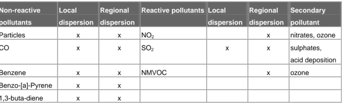
(8) to pollutants with a local dispersion and for pollutants with a regional dispersion. Hence, the total cost due to a pollutant is the sum of the local and the regional cost adjusted for double counting. To value effects of eutrophication and acidification the abatement cost method has been applied because of lack of reliable exposureresponse functions7.. 2. Variations of costs in the all-modes study. Most calculations are based on the same models, values and assumptions8 but still the cost per tonne pollutant differs depending on the situation considered. There are two important reasons for this. First of all, the number of persons exposed to a pollutant is important, hence the population density in the area where the impact is influences the results. For local costs it is the population density in the area close to the source while for regional costs it is the population density on a regional, i.e. European, scale. Secondly, the composition and the amounts of pollutants emitted will influence the results. It is reactions between various pollutants that will influence the amount of harmful substances to which people are exposed. The pollutants considered in the estimation are presented in Table 19. We have divided the table into pollutants that involve in chemical reactions and those that do not. It is important to make this distinction since for non-reactive pollutants it is possible to base the cost on kg of the pollutant emitted. For these, the variation in cost per kg is due to where the pollutants are emitted since the cost depend upon the number of receptors (locally and regionally). For pollutants that involve in chemical reactions it is not this simple. The amount and composition of pollutants emitted differs between different vehicles. The ratio between reactive pollutants will determine the amount of secondary substances that are created in the chemical reactions. The implication of this is that for these pollutants pricing should not be based on a uniform cost per kg, as is the current practice. In the table we have also marked weather or not the pollutants have impact on the local or regional scale, or both. Table 1 Pollutants accounted for in the calculation. Non-reactive. Local. pollutants. dispersion dispersion. Regional. Reactive pollutants Local. Regional. Secondary. dispersion dispersion pollutant. Particles. x. x. NO2. CO. x. x. SO2. x. x. nitrates, ozone. x. sulphates, acid deposition. Benzene. x. x. Benzo-[a]-Pyrene. x. x. 1,3-buta-diene. x. x. NMVOC. x. ozone. Because of variation in costs for pollutants that involve in chemical reactions, in most studies the cost per km is given for different vehicle categories. Using this principle would imply a lack of precision if used for pricing. Another possibility is to use some approximation and relate the costs due to secondary pollutants, ozone 7. These estimates should be interpreted as an approximation since the calculations are based on data that does not represent the most up-to-date state of knowledge (Bickel et al, 2003). 8 Some approximations where used in the cost calculations for airports and maritime transport. 9 The impacts that are valued due to each pollutant are described in Bickel et al (2003).. 8. VTI notat 36A-2003.

(9) for example, to the primary pollutants. We have not investigated the possibility and implication of this in this study. In the following discussion of the results in the all-modes study, we will first exemplify the impact of various variables by presenting cost per tonne for NO2 and SO2 for all transport modes. To make comparisons between modes possible, we will use cost per km in this case. Then, in the following section we will concentrate on differences between urban areas in Sweden.. 2.1. Costs due to NO2 and SO2 for all transport modes. In this section we focus on two pollutants, SO2 and NO2, for which we have data for all transport modes. Comparing the cost estimates between modes for NO2 and SO2 emissions highlights a number of issues regarding the calculations. Of these two, only SO2 is considered to have impacts on the local scale. Another aspect that influences the costs is that both pollutants react with other pollutants to form secondary substances that are harmful. These secondary substances are assumed to have an impact on the regional scale. The amount of secondary pollutants will be different for different transport modes due to differences in the composition of the emissions. We will also see that there are differences between the cost per tonne, which can be related to where the emissions occur. In Table 2 the costs for SO2 emissions are reported. In the first column are presented the cost due to local effects. Two effects are accounted for; mortality and morbidity. For mortality the cost is based on the % change in annual mortality rate per µg/m3 in the population exposed to the pollutant while for morbidity it is based on the number of cases per year per person per µg/m3. Hence the population density in the area where the impact is influences the results. Table 2 Cost for SO2 emissions. Local. Regional. Total. (Eur/tonne). Emitted. Total cost. Mileage. Cost/km. (Tonne). (Eur). (Million km). (Eur/km). Urban roads Gasoline cars. 522. 2113. 2635. 182. 478871. 19920. 0.00002. Diesel cars. 522. -1880. -1358. 12. -15992. 2640. -0.00001. Buses. 522. -5858. -5336. 8. -43647. 490. -0.00009. HDV. 522. -4928. -4406. 18. -78938. 1000. -0.00008. Gasoline cars. 255. 4147. 4402. 127. 558437. 35250. 0.00002. Diesel cars. 255. -1568. -1314. 12. -15742. 4650. 0.00000. Buses. 202. -4102. -3900. 6. -23672. 680. -0.00003. HDV. 202. -3891. -3689. 69. -254835. 4500. -0.00006. Diesel freight trains. 126. -9072. -8946. 0.7. -6252. 3.5. -0.00179. Diesel passenger trains. 142. -16308 -16166. 0.4. -6504. 9. -0.00072. Airports. 840. 1041. 1881. 94. 176742. -. -. Maritime. 366. 659. 1025. 349. 357452. -. -. Extra-urban roads. Other modes. VTI notat 36A-2003. 9.

(10) As expected, the cost is related to where the pollutant is emitted. The cost is lower on extra urban roads and for diesel trains since they mainly travel outside the urban areas. The cost is higher for the scenario covering all airports than the urban roads scenario. This is due to the different shares of pollutants emitted in densely populated areas. 62% of the total emissions in the airport-scenario are from Arlanda and Bromma that are located in densely populated areas. To be noticed is that the local cost due to maritime transport is higher than for other modes that travel in more densely populated areas. The maritime estimate however, should only be considered as an approximation since the spatial resolution used in the calculation is low compared to the other modes. That costs are lower for buses and HDV than cars that are driven on extra urban roads is presumably because cars to a larger extent travel in more populated areas. A somewhat counterintuitive result is found in the second column where the estimated costs for regional dispersed pollutants are presented. For all diesel vehicles we get a negative estimate. This is due to the chemical reactions that take place between NO2, SO2 and NH3. The outcome of the chemical reactions depends upon the ratio between NOx and SO2 emitted. For diesel vehicles this ratio is much higher than for gasoline vehicles. The negative cost occurs because, compared to the reference scenario used in the calculations, less amount of ammonium sulfates is formed and hence the damage due to this pollutant is reduced (see Bickel et al. 2003, for details). That the negative cost is lower on extra urban roads is because the ratio between NOx and SO2 is different. For diesel trains it is interesting to compare the results for passenger transport with those for freight since most of this traffic occurs in extra-urban areas but where the actual emissions occur and the composition of the emissions is somewhat different. What we find is that both the local and the regional cost estimates differ. Diesel freight trains have slightly lower costs for local effects but a considerably lower negative cost for regional effects than do passenger trains. At least part of the explanation for this is the geographical location of the emissions. For diesel passenger trains 7 % of the emissions are in the north of Stockholm while the same figure for freight trains is 57 %. Turning to the third column in the table we find rather large differences in cost per tonne for the different modes. However, for practical purposes this difference is not that important since the amounts of SO2 emitted for the different modes are small. Using the information in the fifth and sixth row we can calculate the cost per km for the different modes and it is almost negligible. In Table 3 the result for NO2 are presented. We have no local costs reported since no health effects have been verified on the local scale (Friedrich and Bickel, 2001). The reason for this is that the results from the first APHEA project suggested that NO2 is only an indicator for other harmful substances10. Regarding the regional effects we find that the cost is lower in extra urban areas. What can be noticed in this table is that the cost per tonne is higher for diesel passenger trains than for any of the other modes, even for urban traffic. Again this is related to the 10. Maybe this conclusion should be revised in view of the findings in APHEA2. APHEA stands for Air Pollution and Health: A European Approach. Bertil Forsberg (2002), who is a member of this research project, has discussed this issue in a paper prepared for SIKA. His conclusion in that report is that there might be correlation between NOx and other harmful substances such as particles. Hence, he recommends that the ER-coefficients for acute mortality for NOx and particles should either be estimated in the same study or should be included but then directed at different endpoints. He also states that more knowledge on this issue should be available from APHEA2.. 10. VTI notat 36A-2003.

(11) geographical distribution of the emissions. Regarding the cost for emissions on open sea is not much lower which is probably due to the larger part of these emissions occurring in the south of Sweden, close to populated areas. Concerning the cost per km we find that the cost is highest for diesel trains which implies that the amount of NO2 emitted per km is comparatively high. Cost for NO2 emissions.. Table 3. Local Regional. Total. (Eur/tonne). Emitted (Tonne). Total cost Mileage (Eur). Cost/km. (Million km). (Eur/km). Urban roads Gasoline cars. 0. 1464. 1464. 18123.4 26537152. 19920. 0.0013. Diesel cars. 0. 1424. 1424. 3272. Buses. 0. 1424. 1424. 5085. 4661145. 2640. 0.0018. 7238990. 490. 0.0150. HDV. 0. 1423. 1423. 9682 13774235. 1000. 0.0140. Gasoline cars. 0. 1453. 1453. 27720 40266598. 35250. 0.0011. Diesel cars. 0. 1391. 1391. 4650. 0.0009. Buses. 0. 1381. 1381. HDV. 0. 1376. 1376. Diesel freight trains. 0. 1042. 1042. Diesel passenger trains. 0. 1681. 1681. Airports. 0. 1305. 1305. Maritime. 0. 1298. 1298. Extra urban roads. 3126. 4349260. 3006. 4151552. 680. 0.0061. 32596 44860960. 4500. 0.0100. 988128. 3.5. 0.2800. 458. 769412. 9. 0.0850. 1032. 1346531. -. -. 18949 24604154. -. -. Other modes. 2.2. 948. Costs on urban roads. The costs for emissions on urban roads have been calculated for different vehicle categories in every urban area in Sweden, i.e. accounting for geographical distribution of the emissions. The cost for each area and each vehicle category are then added to obtain the total cost for all urban areas. We use this figure to calculate the average cost per km in urban areas in Sweden, hence a weighted average of the costs in all urban areas11. Since there are a large number of small towns in Sweden the average population in urban areas is only 3839 inhabitants while the average population density is 1425 inhabitants/km2. The population in Stockholm amount to 16% of the population in urban areas and has the highest population density, 3233 inhabitants/km2, of all urban areas. Since the total km (and emissions) in each urban area in our calculations are related to the population, Stockholm also accounts for 16% of the total km driven in urban areas. Hence, the cost per km in Stockholm will strongly influence the average cost per km. Details regarding the calculations of the emissions can be found in Johansson and Ek (2003). They also discuss how the emissions that we have assumed for each urban area can differ from the actual emissions.. 11. To be remembered in this discussion is that generally how we calculate an average will influence the average value. In the case of population density, summing the total population and dividing by the total area will not give the same result as if we calculate the population density for each area and then sum these. Therefore, our average cost per tonne for urban areas will not be correct for an “average” town.. VTI notat 36A-2003. 11.

(12) The cost per km will differ between the different vehicle categories since the amount of pollutants emitted differ. In Figure 2 we present the cost per km for locally dispersed pollutants. The costs are highest for bus and HDV since they have larger specific emissions. Diesel cars in general have higher costs due to the larger amount of particles emitted. Two-wheelers on the other hand have relatively high costs that are related to the emissions of NMVOC (the cancerogenic substances considered12). These estimates however are valid for the average vehicle in the categories used. Emissions also vary between vehicles in a certain category. There are for example new diesel vehicles with particle emissions per km that are lower than those for the average gasoline vehicle (see appendix 1). For these vehicles the cost per km would be lower than for gasoline vehicles. 0,014. 0,012. 0,01. 0,008 EUR/km. NMVOC CO S02 PM2,5+DME. 0,006. 0,004. 0,002. 0 buss. Figure 2. HDV. Diesel cars. Gasolin cars. Two-wheelers. Costs for locally dispersed pollutants (Eur/km).. The average costs per km for regional effects for the different vehicle categories and pollutants in urban areas are presented in Table 4. Again the costs for the various pollutants are in general higher for bus and HDV. To be noticed in the table is that the abatement cost estimates account for a large share of the total estimated cost for all vehicles except two-wheelers. A surprising result is that abatement cost estimates due to acid deposition are only given for HDV and gasoline cars. These two modes have in common that they have the highest total NOx emissions. Abatement costs only arise after a certain threshold level and this limit is only passed by these two vehicle categories. How this result should be interpreted in practice needs further investigation.. 12. Those accounted for in the calculations are Benzene, Benzo-[a]-Pyrene and 1,3-buta-diene.. 12. VTI notat 36A-2003.

(13) Table 4. Costs due to regionally dispersed pollutants (Eur/km).. Pollutant. Bus. HDV. Diesel cars. Gasoline cars. Two-wheelers. PM 2.5 + DME. 0.0026. 0.0030. 0.0010. 0.0001. 0.0006. Ozone. 0.0089. 0.0083. 0.0011. 0.0016. 0.0026. NO2. 0.0148. 0.0138. 0.0018. 0.0013. 0.0001. SO2. -0.00009. -0.00008. -0.000008. 0.00002. 0.000003. Acid dep.. 0.0007. 0.0006. 0.00008. 0.00007. 0.000005. 0.0000001. 0.00000009. 0.00000003. 0.0000009. 0.0000007. 0.00005. 0.00005. 0.000003. 0.00003. 0.00009. 0.0011. 0.0012. 0.0003. 0.0006. 0.0002. Cost/km. 0.0282. 0.0267. 0.0044. 0.0057. 0.004. NO2 (Abatement cost). 0.0258. 0.0216. 0.0036. 0.0017. 0. CO NMVOC (Benzene, BaP, Butadiene) Fuel prod Impact pathway. Acid dep. (Abatement cost) Total Cost/km. 0. 0.0257. 0. 0.0033. 0. 0.0540. 0.0740. 0.0080. 0.0090. 0.0040. 48%. 64%. 45%. 34%. 0%. (Abatement) Share of cost. In the project we have also calculated the cost for two specific urban areas in Sweden; Stockholm and Skellefteå. Some data on the differences between these areas are presented in Table 5. The population density is highest in Stockholm and hence we can expect higher estimates for pollutants with local impact in this area. The kilometers driven by gasoline cars relative to diesel cars are the same for all cases because of our assumption regarding the emissions in urban areas. Stockholm account for about 16 % of the total km driven in urban areas while Skellefteå only account for 0.4 %. Table 5. Statistics for urban areas. Population. All urban area Stockholm Skellefteå. 7462943 1212196 31742. 2. Area (km ). Population density. 5235 375 22. Vehicle km. Vehicle km. gasolin cars. diesel cars. 2. 20260 million. 4130 million. 3233 person/km. 2. 3292 million. 671 million. 1462 person/km. 2. 86 million. 17.5 million. 1425 person/km. For Stockholm and Skellefteå the cost calculations where made for two vehicle categories; diesel vehicles and gasoline vehicles. To be able to compare the estimates for the average cost/km in urban areas with these two cases we have used the cost estimates for the specific vehicle categories, summed them up and divided them by the kilometers driven for the whole category. These cost estimates for each pollutant are presented in Table 6.. VTI notat 36A-2003. 13.

(14) Table 6. Average costs for gasoline and diesel vehicles in urban areas (Eur/km). PM2.5+ Ozone NO2. NO2 *. SO2. Acid dep. Acid. DME. CO. NMVOC Fuel. dep. *. prod.. Gasoline vehicles Local. 0.0004. 0. 0. 0 0.000005. Regional. 0.0001 0.0016 0.0013 0.0017. 0. 0. 0.000004. 0.00002 0.000007. 0.0032. 0.000001. 0. 0.0000002. 0.0001. 0. 0.00007 0.0006. Diesel vehicles Local. 0.0063. Regional. 0.0017 0.0038 0.0062 0.0106. 0. 0. 0 0.000005 -0.00004. 0 0.0003. 0.0062 0.00000006. 0.00008. 0. 0.00002 0.0006. *Abatement cost estimates.. Since diesel vehicles include HDV and buses the cost per km is much higher for diesel vehicles. To see how the cost for these categories change as we move from one area to another we have calculated the relative difference between the average estimates and the estimates for the case studies (in per cent). The results of these calculations are presented in Table 7. Table 7. Comparison average cost urban areas and case specific costs. PM2.5 Ozone NO2. NO2 *. SO2. +DME. Acid. Acid. CO. dep.. dep. *. NMVOC Fuel production. Gasoline vehicles Stockholm Local Regional. 186% 57%. 186% 100%. 91%. 168% 200%. 89%. 154%. 186%. 186%. 57%. 57%. 78%. 78%. 41%. 41%. 186%. 186%. 57%. 57%. 78%. 78%. 34%. 34%. 100%. Skelleftea Local. 78%. Regional. 41%. 78% 100%. 29% 3989%. 27%. 24%. 0%. 100%. Diesel vehicles Stockholm Local Regional. 186% 57%. 186% 100%. 89%. 132%. 74%. 83%. 100%. Skelleftea Local. 78%. Regional. 34%. 78% 100%. 29%. 0%. 6%. 25%. 0%. 100%. *Abatement cost estimates.. A general result is that the costs for the (non-reactive) pollutants that have local impact change by the same amount. They increase for Stockholm and decrease for Skellefteå. The main reason is differences in population density. Twice as many people will be exposed to the pollutants emitted per km in Stockholm as in Skellefteå. However, the cost estimate decrease for Skellefteå although they have a slightly higher population density than the average for urban areas. This reveals that it is not straightforward to compare average cost estimates with cost estimates for specific studies. The average will be influenced by the geographical location of the emissions where meteorological conditions and population density will be different from those in the case study. 14. VTI notat 36A-2003.

(15) For the pollutants with regional dispersion we do not have the same result. For ozone the cost estimate is the same irrespective of where the emissions occur. The reason is that the calculation of ozone formation is based on EMEP country-togrid matrices, so the results for a country are mainly the same. For particles, CO and NMVOC (the cancerogenic substances considered), which do not involve in chemical reactions, the cost changes by the same amount (shaded areas in the table). The costs decrease both for Stockholm and Skellefteå, which is probably due to the geographical location of these two cities, close to the Baltic Sea. The explanation for the lower cost estimates for regional impacts for NO2 and acid deposition and the higher cost for SO2 regional for gasoline cars in Stockholm are related to a number of factors such as differences in geographical location, background concentrations, air chemistry etc and it would require a more thorough analysis to fully understand the impact of each parameter. The striking result in this table is the much higher abatement cost estimate for NO2 for gasoline cars in Skellefteå. In this project we have not studied the models underlying the calculation of abatement costs. This result however indicates that such investigation is needed. The effect of these differences on the cost/km are presented in Table 8. This table reveals that the cost varies for both locally and regionally dispersed pollutants. For local effects the cost is about twice as high in Stockholm as the average for urban areas while for regional effects the cost appears to be lower in the north of Sweden. The result for gasoline vehicles is uncertain due to the very high abatement cost estimate for NO2 in Skellefteå. The conclusion from this is that costs in urban areas should be differentiated according to local conditions but also based on the geographical location within Sweden. Table 8. Average km cost for urban areas and case specific km costs (Eur/km). Gasoline. vehicles. Local. Regional 0.00861. Total. Average urban area. 0.00056. Stockholm. 0.00104. Skellefteå*. 0.00043. 0.00261. 0.0030. Diesel. vehicles. Local. Regional. Total. 0.0092. 0.00642. 0.02935. 0.0358. 0.01133. 0.0124. 0.01196. 0.02512. 0.0371. 0.07030/. 0.0707/. 0.00500. 0.00685. 0.0118. * We report the cost with/without the abatement cost estimate for NO2.. 2.3. The general assumptions and Swedish conditions. The basic assumptions in the Impact pathway approach have not been adapted to Swedish conditions other than that the values applied to different effects have been adjusted for income differences according to the conventions in the UNITE project13. This is not because we expect that the assumptions are always valid for Swedish conditions but a deliberate choice in order to make comparison with other studies more straightforward. As will be evident from the next section, where the results from the all-modes study are compared to those in other studies, there are a number of modifications that can be done to the Impact pathway approach. Each modification makes it difficult to fully understand and evaluate differences in estimates. There are however, in every step of the chain, questions 13. The part of the modeling that is specific for Swedish conditions is the modeling of the emissions, the meteorological conditions and the population density.. VTI notat 36A-2003. 15.

(16) regarding the validity of the assumptions for Swedish conditions and we will briefly highlight some of them and their possible implications for the results. Further research will have to explore if some of them should be accounted for in future work. Starting with the emission modeling there are a number of factors that can influence the amounts of pollutants emitted per vehicle kilometer (vkm). With more pollutants emitted the cost will increase and hence it is important to get accurate figures. One obvious example where Swedish conditions are different from the European average is the amount of cold starts for road vehicles. These increase the content of some pollutants in the emissions and hence increase the costs. Since we have included this impact in our emission modeling, the cost estimates for an average urban road in Sweden should be somewhat higher than for a road in similar circumstances in Europe. Another aspect that have influenced the results in the all-modes study is that the sulphur content differs between Sweden and Europe. The second step of the chain is the dispersion and exposure modeling. The level of detail in this step would also influence the cost estimates. The current practice for calculating exposure in Sweden in urban areas is a formula based on population and the meteorological conditions in different parts of the country. The formula includes a “ventilation factor” which is 1 at the southern coast of Sweden and 1.6 in the inland in the north (Leksell, 1999). This as a consequence of the fact that the further north we get the more stable meteorological conditions we have. In wintertime we have cases of inversion. This results in higher concentrations on these occasions and hence higher exposure and, presumably, higher costs. In the all-modes study the dispersion modeling is based on annual average meteorological conditions including wind speed. The question is if this approach also accounts for the presumably higher exposure in the north of Sweden that are due to the more stable climatic conditions. If not, adaptations of the dispersion modeling would be required. Based on the exposure, the next step in the chain is to estimate the impact on the population. Here a common set of exposure-response functions are used. In some cases they apply to the whole population while in other cases they apply only to a fraction, elderly or asthmatics for example. To be correct, the calculations should be based on these groups share in the population where the calculations are performed. This has not been accounted for in the all-modes study. Furthermore, the generalization of ER-functions from one area to another is not obvious. According to Forsberg (2002) preliminary results from APHEA2 indicates that the ER-koefficient in some cases are higher for Stockholm than the average in the study. This might also be an issue in the estimation of impacts on crops. For ozone the ER-functions is based on a “critical loads” standard measure (the 40 AOT). The question has been raised if this is appropriate for Swedish conditions with our long summer days (Munthe et al., 2002). A higher ERcoefficient of course implies higher cost estimates. Another issue regarding the assessment of impacts is the calculation of life years lost for acute and chronic mortality. In the all-modes study this is based on “an average” of the survival probabilities in Germany, Italy, the Netherlands and the UK. This “average” might be higher or lower than for Sweden. The final step in the Impact pathway chain is the valuation of the effects. In the all-modes study the values have been adjusted to account for the income level in Sweden. Other modifications could however be considered appropriate. The 16. VTI notat 36A-2003.

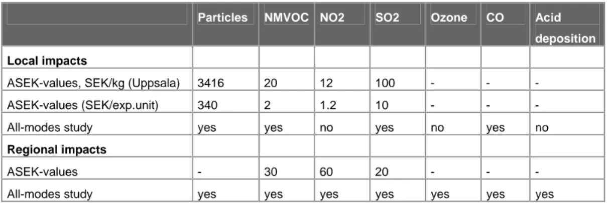
(17) valuation of life years lost is for example derived from the value of a statistical life (VOSL). If this is different from that used in the all-modes study this would influence the results. The same applies to the valuation of morbidity effects. The values used in the all-modes study are derived from European studies. Similar studies have only recently been performed in Sweden. Higher or lower values of course imply higher or lower estimates. Another issue is that the UNITE convention, which is the basis for the values used in the all-modes study, imply factor prices. Usually we value things in market prices since this is the value that individuals reveal. The use of factor prices implies a reduction in the value of about 20 %.. 3. Cost estimates in other studies. Although all the calculations in the all-modes study were based on the same approach, we have seen that the cost estimates per tonne emitted for the pollutants vary depending on where the emissions occur and by what mode. The problems involved in making comparisons increase when we want to understand how these results differ from those obtained in other studies. As discussed in the previous section, there are a number of factors that will result in differences: – the emission modeling – the dispersion modeling – the pollutants and the endpoints considered – the exposure-response functions – the values attached to different endpoints. Over the years a number of cost estimates that more or less relies on the Impact pathway approach developed in the ExternE projects have been calculated. In the following we will review and compare our estimates with those derived in some other studies. The first comparison concerns the estimates currently used in Sweden that in part were based on an earlier version of the ExternE-approach. Secondly, we will compare and discuss our results and those in two recent Swedish marginal cost case studies. Finally, we will highlight some of the differences between the assumptions used in our study and those underlying the BeTa-estimates that are presented by DG Environment (Holland and Watkiss, 2002). This overview will again reveal how different assumptions in the calculations preclude simple comparisons.. 3.1. The ASEK-values. In transport investment analysis in Sweden a common set of prices are used to value benefits and costs, the so-called ASEK values. The cost estimates used for air-borne pollutants are presented in Table 9. These values are the result of a study undertaken by Leksell (1999), which was commissioned by SIKA. As in our study there are cost estimates for pollutants with local impacts and for those with regional impacts. The estimates for the local scale are partly based upon the estimates in the ExternE-approach from 1995 and 1998 while those for the regional scale are based on abatement costs. The cost per kg is dependent upon individuals exposed and we have used the cost estimates for Uppsala (SIKA,. VTI notat 36A-2003. 17.

(18) 2002, page 113)14. In the table are also added the pollutants that are included in the calculations in the all-modes study. The pollutant NMVOC is a cause for confusion since it is the name for a group of pollutants. Some of them are found to cause cancer and are therefore valued. But NMVOC is also valued because it is one of the pollutants behind the formation of ozone. The effects accounted for in ASEK on the local scale are the increased risk for cancer while it is unclear what the basis is for the cost estimate on the regional scale (cancer and/or ozone). In the Impact pathway approach some specific NMVOC are accounted for since they cause cancer while ozone is treated as a separate pollutant that is only accounted for on the regional scale. Table 9. Air pollutants accounted for in ASEK and the all-modes study. Particles. NMVOC NO2. SO2. Ozone. CO. Acid deposition. Local impacts ASEK-values, SEK/kg (Uppsala). 3416. 20. 12. 100. -. -. -. ASEK-values (SEK/exp.unit). 340. 2. 1.2. 10. -. -. -. All-modes study. yes. yes. no. yes. no. yes. no. ASEK-values. -. 30. 60. 20. -. -. -. All-modes study. yes. yes. yes. yes. yes. yes. yes. Regional impacts. The table reveals that the pollutants accounted for in these studies differ. On the local scale the most important difference is the treatment of NOx. There are two problems related to the valuation of this pollutant. First of all, there is a complicated chemical reaction between NOx and ozone that is influenced also by meteorological conditions and the ambient concentration of these and other substances. Hence, in some circumstances the concentration of one pollutant can increase while the other decrease and in other cases they can both increase (Friedrich and Bickel, 2001; Lindskog et al., 2002). Since general predictions are difficult to make, in the Impact pathway approach they do not account for this chemical reaction in the dispersion modeling on the local scale. Another problem is that the scientific evidence on the effects of NO2 are unclear (see footnote 10). Therefore, in the ExternE projects they have come to the conclusion not to include the valuation of NO2 on the local scale. Leksell (1999) also came to the conclusion that the effects of the chemical reaction were difficult to quantify. He raised the questions that maybe the effects of increases/decreases in ozone and NO2 could be considered to cancel out and hence no valuation was needed. He also discussed the lack of scientific evidence for the impact of NO2. The final result of this discussion was that only directly emitted NO2 should be valued. NO2 is also involved in the chemical reaction in the creation of ozone. As for NMVOC, it is unclear how the cost for regional dispersion of NO2 relates to the impact of ozone in the values used by Leksell (1999). Of the ASEK-values only those for particles are truly based on the Impact pathway approach, i.e. based on the assessment of different health (and other 14. Our reason for choosing the values for Uppsala is that these correspond well to the average cost for all urban areas that we obtain when using the ASEK-values.. 18. VTI notat 36A-2003.

(19) effects) that are given a value. The assumption behind these cost estimates are however somewhat different from those in the all-modes study. One difference is that the ER-coefficient used by Leksell is higher. This is in accordance with the assumptions in the earlier ExternE projects. In the present version of the Impact pathway approach the coefficient is scaled down by a factor three because the studies from which the coefficient is collected concerns conditions in the USA, which are not considered to be valid for European conditions (Friedrich and Bickel, 2001). Another difference is that Leksell (1999) based his calculations on a lower VOSL. Yet another difference is that the estimates in the all-modes study are based on factor prices instead of market prices. To make the cost estimates comparable we have converted the estimates in the all-modes study to market prices and we also present results where we have used the original coefficient for chronic mortality (upscaled) in the calculation15. In Figure 3 we can see the differences between the average cost/km for gasoline car and HDV in urban areas. The ASEK-values are composed of estimates for local effects based upon exposure, and the regional effects based on abatement costs. For the all-modes study we present the estimates from the Impact pathway approach separately for local and regional effects and, in addition, the abatement cost estimates due to acidification and eutrophication. 3. 2,5. SE K /km. 2. Abatem ent cost R egional im pact Local im pact. 1,5. 1. 0,5. 0 A SEK H D V. Figure 3. AS EK G C. H D V upscaled. G C upscaled. HDV. GC. Cost/km for urban areas in ASEK and the all-modes study (SEK).. Even for the upscaled estimates the cost per km is lower in the all-modes study and the main difference is the cost due to local impacts. One reason for this is differences in the values used, and how these values have been derived. In the ASEK-values are included cost due to chronic mortality for SO2 and costs due to soiling from particles as well as effects of NO2. The most influential difference however is not the values used. Instead it is the function used to calculate the impact (specific exposure) in urban areas that gives the much higher cost per kg. As an example, according the formula used by Leksell (1999), 7,2 persons would be exposed to 1 µg of PM2.5 per year per kg emitted in Skellefteå16. For the allmodes study this figure is 0,58 persons per kg emitted, a difference of a factor 12. 15 16. Market prices=1.20*factor prices. 1 EUR= 9 SEK Specific exposure = 0.029*F*√B = 0.029*1.4*√31742=7.233. VTI notat 36A-2003. 19.

(20) The basis for the exposure function used by Leksell (1999) is unclear and we have not been able to further investigate if this represents the most current state of knowledge. We only notice that it is not based on those aspects that are found to be of importance in the all-modes study; population density and meteorological conditions such as wind direction and speed. Concerning the costs for regionally dispersed pollutants, the abatement cost estimates are about the same although the basis for the valuation differs. In total, the costs for regional effects are higher in the all-modes study because we also need to include the costs that are calculated with the Impact pathway approach. Leksell (1999) did a calculation of regional cost estimates for health effects based particle emissions and ozone using the Impact pathway approach. He found that these values were lower than the regional cost estimates that were derived with the abatement cost approach. Since the latter should include all effects from regionally dispersed pollutants, he concluded that it was satisfactory only to use the abatement cost estimates for regional effects. In the all-modes study the abatement cost estimates only concerns effects on the eco-system and hence these should be added to the costs that are calculated with the Impact pathway approach.. 3.2. The Marginal cost case studies in 2002. In 2002, Ekono Elekktrowatt OY in Finland performed two case studies in Sweden. One derived estimates for local maritime transport (Hämekoski et al., 2002) while the other calculated the cost of one specific aircraft in one airport (Otterström et al., 2003). As for the all-modes study, these studies are based on UNITE conventions, and the values used in the UNITE project, which simplifies the comparison. These studies however differ in other respects. While the allmodes study is based on total emissions during a year for each transport mode, these studies are so called marginal cost studies. Therefore the basis for the estimation is the emissions from one type of transport mode in a certain situation. This does not mean however that the amount of emissions needs to be particularly small. The assumption in both studies is that the transport mode makes one trip every hour during a whole year17. Yearly emissions are the basis for the calculation since many other parts of the calculation are based on the use of yearly data. The composition of emissions however may be different from those in the all-modes study and this could influence the chemical reactions and hence the cost estimates. The latter however is not a problem for comparison since a detailed dispersion modeling on the regional scale is not performed in these studies. It is only on the local scale that the Impact pathway approach is implemented. Hence, on the local scale a thorough dispersion modeling is undertaken to assess the impacts. This is the second major difference between these case studies and the all-modes study. Since the population density and meteorological conditions in the areas considered in these studies may be different from those in the all-modes study, differences in cost estimates can result. Furthermore, costs due to regional impacts are based on a cost per tonne pollutant emitted from a Finnish maritime case study in the UNITE project. Therefore they do not vary between different regions as 17. In the case of the maritime study, it was assumed that one ship leaves port every hour and the emissions for one year was used in the calculations. It turns out that this assumed ship flow is between 10 % and 30 % of the actual ship flow on the routes considered.. 20. VTI notat 36A-2003.

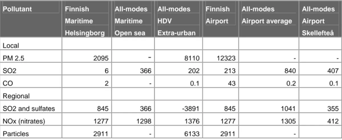
(21) they should depending on differences in population density. They may also differ from those costs estimated in the all-modes study because of differences in other relevant conditions between Sweden and Finland. The costs due to particles from maritime and aviation were not calculated in the all-modes study due to missing data. Therefore we have included the values for HDV that are driven in extra urban areas for comparison to maritime transport. We have also included the costs for the airport in Skellefteå, in addition to the average cost for all airports. The route chosen for comparison in the maritime study is that to Helsingborg since it is a long route that passes along the coast. Hence, the population density along the route should not be that small. The figures are presented in Table 10. For PM2.5 and SO2 the costs are lower in the Finnish maritime study in the case of local effects. This is also the case for SO2 emissions from airports. Hence, although it is problematic to draw some conclusion from the comparison between maritime transport and HDV, these differences raise the question of the possible impact of local dispersion modeling. Is it possible that the dispersion modeling in the Finnish studies is more detailed regarding wind conditions and that, therefore, the exposure becomes less in the studies. That they, despite that, gets a higher cost due to CO seems to be explained by a difference in the population that is accounted for. In the Finnish study CO is assumed to affect the whole population but in the all-modes study it is only the elderly. Table 10. Costs in the case studies and the all-modes study (Eur/tonne).. Pollutant. Finnish. All-modes. All-modes. Finnish. All-modes. All-modes. Maritime. Maritime. HDV. Airport. Airport average. Airport. Helsingborg. Open sea. Extra-urban. Skellefteå. Local 2095. -. 8110. 12323. -. -. SO2. 6. 366. 202. 213. 840. 407. CO. 2. -. 0.1. 43. 0.2. 0.1. 845. 366. -3891. 845. 1041. 355. NOx (nitrates). 1277. 1298. 1376. 1277. 1305. 412. Particles. 2911. -. 6133. 2911. -. PM 2.5. Regional SO2 and sulfates. Regarding the pollutants with regional dispersion it is difficult to draw firm conclusions. The cost estimate for NO2 and SO2 seems to be in the same range as the cost in the all-modes study. It appears that they are somewhat lower than the estimates in the south of the country but high if we were to use them for emissions in the north. For particles the comparison seems to indicate the same, i.e. that the estimate used is somewhat low for emissions in the south of the country. Based on these comparisons our conclusion is that the main question raised by the results in the finnish studies is the impact of local dispersion modeling.. 3.3. The BeTa-estimates. Netcen (Holland and Watkiss, 2002), on the commission of DG Environment, has prepared a database containing cost estimates that can be used to calculate total costs for various air pollutants in different circumstances. The basis for this. VTI notat 36A-2003. 21.

(22) database is an earlier version of the Impact pathway approach developed in the ExternE projects. To compare all our estimates with those in this database are not possible, but the following comparisons reveal quite large differences in the estimates, which of course raises questions. The figures in Table 11 for the Beta estimate are based on the recommendations in the report and the estimates from the all-modes study concern gasoline vehicles. The first thing to notice in the table is the large difference in cost between a small and a large city with the BeTa-estimates for local effects of PM2.5 and SO2. We do not get this large difference between our case studies. According to the recommendations in BeTa, the cost per tonne should increase linearly with population size up to cities with a population of 500 000 and then somewhat less. This is not a relationship that we find. The cost per tonne pollutant emitted in Stockholm is only twice as high as in the city of Skellefteå (where the population is 40 times lower). One explanation for this is that the cost per tonne is mainly related to the population density, which is about twice as high in Stockholm. It is the total cost for the emissions that is related to the size of the population. Our result raises questions regarding the underlying assumptions behind the recommendations in BeTa. Table 11. Cost per tonne in the BeTa and the all-modes study (Eur/tonne).. Pollutant. BeTa. BeTa. All-modes. All-modes*. All-modes. All-modes. Skellefteå. Stockholm. City of. City of. Average for. Average for. City of. City of. 100 000. 1 000 000. urban area. urban area. 31 742. 1 212 196. Local PM 2.5. 33 000. 247500. 20964. 25157. 16320. 39072. 6 000. 45000. 522. 626. 407. 973. SO2 and sulfates. 1700. 1700. 2108. 2530. 579. 4218. NOx (nitrates). 2600. 2600. 1464. 1757. 421. 1327. Particles. 1700. 1700. 5543. 6652. 2256. 3173. SO2 Regional. * Market prices. Another difference is that the estimates for pollutants with local dispersion are lower in the all-modes study. To understand the reason for this difference we have compared the assumptions and found that they are different. First of all, most values used in BeTa are based on the version of the ExternE-approach that are presented in Friedrich and Bickel (2001). These values are higher than those used in the all-modes study since they are market prices. Another reason that can explain the difference is the approach used for the valuation of mortality. In BeTa they have used the EC DG Environment’s preferred approach to economic valuation of mortality (EC DG Environment, 2000) which is based on the value of a statistical life (VOSL) instead of the value of life years lost (VOLY). This implies a value for acute deaths of 1 000 000 Euro instead of 131 400 Euro for a life year lost. For chronic deaths the value is 490 000 Euro instead of 76 400 Euro for a life year lost. A shortening of life of less than one year among elderly are assumed in the first case, according to EC DG Environment, while five years are assumed for deaths due to chronic mortality. Since the valuation of mortality is an 22. VTI notat 36A-2003.

(23) important, and unresolved, issue concerning the economic valuation of health effects, we will describe the main differences between the two approaches in the following (for a detailed discussion see Friedrich and Bickel, 2001; Rowlatt et al., 1998; Pearce, 2000). As presented in Bickel et al. (2003) the measure used in the Impact pathway approach is years of life lost, both to estimate the costs of acute and chronic mortality (deaths that occur with latency). The reason stated for using this approach is that it agrees with the effects that are quantified by the epidemiological exposure-response functions. To be able to value years of life lost the value placed on an additional year is needed. This value is derived from an estimate of the VOSL, which is converted into a time stream of constant VOLYs. The simplest approach is to regard VOLY as the annuity which when discounted over the remaining life span of the individual would equal the estimate of VOSL. In some circumstances this estimation is based on the information regarding traffic accidents; the VOSL used and the average remaining life expectancy for those who die in these accidents. In the Impact pathway approach the basis is instead survival probabilities for the EU population (see Friedrich and Bickel, 2001 and Bickel et al., 2003, for details). One objection raised against the VOLY approach is that it does not have a theoretical basis (Pearce, 2000). Another is that it does not agree with empirical findings. A constant value for each year is assumed which implies that the VOSL progressively decline with age. Empirical findings instead suggest a peak for VOSL in middle age (Rowlatt et al., 1998; Pearce, 2000). There are however also problems related to the use of VOSL. To use this approach the exposure-response functions need to be converted so that they estimate fatalities in the population instead of years of life lost. The conversion used in BeTa is that a death due to chronic effects equals five years lost (although 10 years have been used in other circumstances). For acute effects the conversion factor is not specified. Furthermore, discounting is needed to obtain the present value of chronic mortality. In BeTa the VOSL for acute effects has been discounted at a rate of 4% to obtain the VOSL for chronic effects. Hence, in either case the valuations are based on a number of assumptions. We have not been able to trace out the exact implications of these differences in the valuation approaches for the results. Presumably they are the reason for the higher cost estimates for PM2.5 and SO2 for local effects. It appears that the same exposure-response function is used for acute mortality in BeTa as in the all-modes study18. If this is the case but the value used in BeTa is 1 million instead of 131 400, this would explain the higher value for SO2 emissions. Higher estimates is however not a general result. Comparing the estimates for regional dispersed pollutants we find that the costs for PM2.5 and SO2 are higher in the all-modes study while it is lower for NO2. To investigate the reason for these differences would require information on the underlying dispersion and exposure modeling.. 18. Mail correspondence with Peter Bickel 2003-03-17. VTI notat 36A-2003. 23.

(24) 4. Generalizations of the cost estimates. As discussed in the introduction to this paper, estimates of the external cost of transport air pollution are used in policy work. To evaluate a policy measure, situation specific cost estimates are asked for. The problem in achieving this is the number of variables that influence the cost at a specific moment in time. Even if the Impact pathway approach was used, the estimates would only be approximations. Lack of knowledge regarding underlying relationships impose restrictions on how close the estimates will be to true costs. Currently the estimates from the Impact pathway approach are yearly averages. One reason is that the exposure-response functions for health effects are quantified for yearly exposure. Further development of the approach can give more detailed estimates but this is the current state of the art. However, to use the Impact pathway approach to arrive at cost estimates for each situation is not economically feasible. Hence, it would be useful if estimates in one situation could be generalized to other situations but unfortunately this is not straightforward. One objective in the UNITE project was to develop models for generalizations but it is concluded that further studies are needed before this can be achieved (Bickel et al., 2002). Therefore, in this sections we will discuss what are the causes for variations in the estimates and what needs to be accounted for when transferring the estimates from one situation to another. This will provide some answers to what information the estimates in the all-modes study can provide regarding costs in other situations.. 4.1. Situation specific determinants. How the results from the Impact pathway approach can be generalized has been addressed in the UNITE project based on the finding in a number of marginal cost case studies (Bickel et al., 2002). Their conclusion is that a direct transfer of costs due to air pollution cannot be recommended and that a generalization methodology for air pollution should account for: – the local scale conditions (population density and local meteorology), and – the regional scale cost per tonne of pollutant emitted in a certain area. Furthermore, while the Impact pathway approach as such can be generalized they conclude that some inputs to the model need to be situation specific. This concerns emission factors for vehicle fleets, inputs to dispersion models and monetary values for health effects. We will discuss each of these in turn. 4.1.1 Emissions The calculations in the all-modes study are based on modeled emissions. These emissions will differ from actual emissions in specific situations and hence the cost estimates will be approximations to true cost. More accurate cost estimates can of course be obtained with more detailed emission models. For our purpose, the level of differentiation chosen was to distinguish between emissions within and outside urban areas as well as for different modes. Furthermore, as will be discussed in the next section, the cost for a pollutant is determined by where the emissions takes place. Therefore, when we discuss generalizations in this section. 24. VTI notat 36A-2003.

(25) they relate to the possible generalizations between different vehicles in a specific situation (ceteris paribus). The emissions considered in the calculation will depend on the vehicle considered. Marginal cost case studies consider the emissions from one specific vehicle while the level of detail in the all mode study is average emissions for a vehicle category. This however does not seem to cause different estimates for cost per tonne for non-reactive pollutants (particles, CO and specific NMVOC). The estimated costs for these pollutants are the same irrespective of if the calculations were related to diesel cars, gasoline cars or buses for example. Hence, for these pollutants the estimates in the all-modes study should be possible to use to calculate the cost for a specific vehicle, at least for local impacts. Instead, there are problems related to those pollutants that involve in chemical reactions (NOx, SO2 and NMVOC). Since these impacts are on the regional scale, this prevents the transfer of the cost per vehicle category for regional effects to specific vehicles. To calculate the cost for these emissions it is the final pollutants that are of importance (NO2 and nitrates, SO2 and sulphates and ozone). The formation of these pollutants are among other things determined by the composition of the emissions. According to our results it is important to differentiate the cost between gasoline vehicles and diesel vehicles and the cost also vary between different diesel vehicles. Further problems is that the formation of secondary pollutants is influenced by background concentrations. For these reasons the cost cannot be related to the amount of the primary pollutant that is emitted. 4.1.2 Dispersion modelling For a given pollutant, the cost will vary depending on where the emissions take place. On the local scale we have different costs for Skellefteå and Stockholm because the population density differs between these two cities. Higher population density implies that more people will be exposed to every tonne pollutant that is emitted. More people exposed results in higher impact and therefore higher costs. The exposure however is modified by the wind conditions in the area where the emissions take place. With more stable conditions we get higher exposure. This can explain why we do not obtain the same cost per tonne particles emitted for all urban areas and Skellefteå although the populations density is about the same. Differences in population density are also one reason for estimating separate costs for transport within and outside urban areas. The local costs will be much lower for vehicles traveling outside of urban areas. For pollutants with a regional impact population density and wind speed also influence the estimates. The wind direction determines where the exposure will take place. If the wind transports the pollutants to densely populated areas in Europe, the cost will be higher. Therefore, for costs due to regional impacts the geographical location of the emissions is of importance. In the all-modes study we find that the regional costs in Skellefteå are lower than the average costs for all urban areas and Stockholm. Hence, some differentiation within Sweden is required for regionally dispersed pollutants. The implication of this is that it is problematic to transfer the estimates in the all-modes study to other situations. Further research into the area of dispersion and exposure modeling on the local scale seems to be required before these estimates become transferable. Such research is also warranted since we find that. VTI notat 36A-2003. 25.

(26) these estimates heavily influence the final cost estimates. The formula used by Leksell (1999) to calculate exposure gives much higher values than those in the all-modes study while the reason for the lower estimates for local impacts in the finnish studies (Hämekoski et al, 2002; Otterström et al., 2003) could be the dispersion models that they use. For pollutants with regional impact the dispersion modeling seems to be more complicated but the effects on the other hand occur in a larger area. Hence many factors influence the final estimate and therefore less detail regarding the generalization seems to be warranted. The information that is obtained from the estimates in the all-modes study is what aspects that are important to consider in the differentiation of costs and also for which pollutants it is important to do so. For the pollutants accounted for on the local scale, at least population density and wind direction should be considered. This means differentiating between different urban areas in Sweden but the implications is also that costs should be differentiated within urban areas and depending on the prevailing weather conditions. For pollutants with a regional dispersion, except ozone, there seem to be differences at least between the north and the south of the country with lower costs in the north. 4.1.3 Effects and values In the UNITE project it is concluded that values should be country specific. In the all-modes study this has been accounted for by adjusting European values for income differences. This again is an approximation needed since no country specific values are available. It would be possible to base the calculations on a country specific VOSL and also for specific values of morbidity. The calculated effects due to a specific exposure is also derived from European averages. The conclusion in UNITE is that exposure-response functions can be generalized. This however is an assumption that can be questioned and that we think need further investigation. Findings in the APHEA2 project indicates that the effects due to a certain exposure can be higher in Stockholm than in other European cities. The share of the population that is susceptible to exposure also seems to vary. In Sweden the share of asthmatics in the population is 8% compared to 3.5% that is the assumption behind the calculations in the all-modes study.. 4.2. Large or small emissions. The definition of marginal external costs is a change in the total external cost resulting from an additional vehicle on a transport route. The marginal external costs from one additional vehicle should be calculated for a single trip on a chosen route segment. With this interpretation the marginal external costs due to air pollution will differ depending on road type, driving behavior, vehicle type, wind speed, wind direction, surface roughness (albedo), population densities along the road etc. Marginal in this sense also implies that the costs are related to one specific moment in time and the background concentrations that prevail in that instance. Hence, if these calculations were performed there would be a difference between costs in one city depending on if it was morning rush hour in summertime or wintertime and whether we looked at an old or a new car, petrol or diesel, with an eco-driver or not, close to an open space or in a narrow street. This, however, is not the interpretation that should be made regarding the marginal cost estimates in the case studies that we have presented. The. 26. VTI notat 36A-2003.

No results found