Cache-Partitioning for COTS Multi-coreArchitecture

(1)

Mälardalen University

Master thesis in Intelligent Embedded Systems

Cache-Partitioning for COTS Multi-core

Architecture

Author: Konstantinos Konstantopoulos Supervisor: Rafia Inam Mohammad Ashjaei Examiner: Prof. Mikael Sjödin

(2)

(3)

Abstract

Multi-core architectures present challenges to execute real-time applications. Concur-rently executing real-time tasks on different cores, can produce negative impact on each others execution times due to the shared resources e.g. shared last-level cache, shared memory bus etc. Shared last-level cache is a resource of cache pollution that negatively impacts the execution times of tasks. In this thesis project we provided support for last-level cache partitioning through the mechanism of page coloring. Using page coloring, the last level cache is divided in multiple partitions. Tasks are allowed to access their own partition only, thus achieving cache isolation. The implementation is done in Linux OS. The aim of the thesis is to incorporate this work with the previous implementation of Multi-Resource Server to achieve task isolation.

(4)

Dedication

(5)

Acknowledgements

I would like to thank all the people involved in this project, and particularly my supervisor Rafia Inam for her valuable guidance.

(6)

List of abbreviations and symbols

COTS . . . Commercial Off-The-Shelf

CMP . . . Chip Multi Processor

CPU . . . Central Processing Unit

DRAM . . . Dynamic Random Access Memory

IPC . . . Instructions Per Cycle

LLC . . . Last Level Cache

LRU . . . Last Recently Used

MRS . . . Multi-Resource Server

NUMA . . . Non-Uniform Memory Access

OS . . . Operating System

PFN . . . Page Frame Number

PGC . . . PaGe Coloring

QoS . . . Quality of Service

RAM . . . Random Access Memory

(7)

SRAM . . . Static Random Access Memory

TLB . . . Translation Lookaside Buffer

UMA . . . Uniform Memory Access

VAS . . . Virtual Address Space

VPFN . . . Virtual Page Frame Number

(8)

Introduction

1.1 Introduction

One of the greatest challenges in real-time systems is to achieve predictable execution of concurrent applications. When multiple tasks execute on the same hardware, there is an inherent competition for shared resources such as the central processing unit (CPU), last-level cache (LLC) and memory. Unbounded access of one task to those resources, affects the performance of completely unrelated tasks, executing on another core, and creates unpredictable execution.

The shift towards multi-core CPUs brought many advances in performance and power efficiency [22]. However, it has also introduced new challenges for real-time systems such as task interference not only on the same core, but also between different cores. Fur-thermore, there is interest to use general purpose operating systems (OS), executing on commercial off-the-shelf (COTS) hardware, something that can offer significant benefits like widespread availability and reduced cost [23]. Unfortunately, most of the consumer grade systems are optimised for performance, and are lacking real-time capabilities and guaranties [24][25].

A previous approach that attempted to address some of these issues is the Multi-Resource Server (MRS) [9]. The MRS can effectively bound the CPU time and memory bandwidth contention but there are more aspects to take into consideration. Most

(12)

mod-ern CPU architectures include cache memory in order to increase performance by keeping the needed data locally into caches. The performance gain of cache memory depends en-tirely on the right data to be in the cache at the right time, something that cannot be guaranteed, and therefore is highly varied from execution to execution. Addition-ally, some of the cache layers are typically shared among multiple cores, causing task interference even if they execute on different cores.

Another common approach is to simply disable caching, thus exchange performance for predictability, but such a trade-off is not always possible [20][21]. It is evident that there is a great need for a mechanism that bounds the stalling time due to cache misses and allows a tighter Worst Case Execution Time (WCET) for real-time tasks executing on COTS hardware.

1.2 Motivation

The research goal of this thesis is to minimise the execution-time variance caused by CPU cache contention of tasks that execute concurrently on COTS multi-core architectures. This will be achieved via a mechanism that is able to partition the cache, and assign different partitions to different processes, and thus preventing contention. Additionally, this mechanism must be integrated into the existing MRS system.

This thesis aims to answer the following questions:

1. Is it feasible to design and implement a cache partitioning mechanism on COTS hardware, on top of Linux and MRS?

2. Will the cache partitioning mechanism, combined with the existing MRS work, provide better execution predictability?

1.3 Scope

(13)

1. Investigate existing cache partitioning methods. Designing a novel method is not required but such a possibility will not be ruled out.

2. The cache partitioning method must be implemented on COTS hardware.

3. The cache partitioning method must be implemented on Linux.

4. The cache partitioning method must be integrated with MRS.

5. The cache partitioning must work on a per-server granularity; a per-server property will determine which cache partition the server tasks will use.

1.4 Contributions

1. Researched existing cache partitioning methods.

2. Reproduced page coloring method as described in PALLOC[10]. However, the current implementation differentiates in tree points:

• In PALLOC the authors are using page-coloring to achieve DRAM memory bank partitioning; In the current work it is used to partition the last level cache.

• Freed pages are re-inserted into the appropriate color index, instead of the buddy system lists. This makes de-allocation and future allocation times more deterministic, at the expense of having a large portion of physical mem-ory fragmented into single-page blocks. This is not a problem for user-space programs but kernel-space requests for contiguous multi-block physical mem-ory could fail.

• The current work utilise the fork-exec technique to assign a cache partition to a process; PALLOC is using cgroups.

3. The cache partitioning mechanism is integrated with MRS in such a way that the cache partitions are just another shared resource that can be managed by the user.

(14)

A tool has been created to simplify the MRS/cache-partitioning configuration via a single JSON file. For comparison, in the existing MRS system the user had to configure three different files, a procedure that is error prone and unintuitive.

1.5 Limitations

During the later stages of the present work, it was discovered that the CPU was prefetch-ing instructions and data into the caches and was distortprefetch-ing the measurements. Prefetch-ing can sometimes be disabled through the BIOS or by settPrefetch-ing special registers, but nei-ther option was available on the given hardware. As nei-there was no alternative hardware available, the experiments were limited to special synthetic workloads that were able to neutralise prefetching by using random reads.

(15)

Chapter 2

Background

2.1 Real-time systems

Real-time is a system that is able to respond to events within a specified deadline. The correctness of the system depends not only on the correctness of the response but also on delivering the response on time. Missed deadlines are highly undesirable and can prevent the system from performing its intended function. As a mater of fact, real-time systems are categorized depending on the degree of tolerance of missed deadlines.

Hard real-time: Systems in this category must absolutely meet each and every dead-line, otherwise their mission will fail. In many cases a failed hard real-time system can cause severe damage and/or loss of life. Nuclear, medical, military, aviation, and aerospace systems are typical examples of hard real-time systems.

Firm real-time: Systems in this category tolerate sporadic deadline misses. Responses after a missed deadline are useless, and too many missed deadlines will partially or completely degrade performance. An assembly line is an example of a firm real-time system. A few misses might start affecting manufacturing accuracy and speed and lead to rejected products, but could still be within acceptable limits; however too many misses will raise quality control issues.

Soft real-time: Similar to firm real-time but more tolerant. Response after a deadline miss might still hold some value. For example a video teleconference system still retains

(16)

value even though there might be delays in the sound or missed frames in the video.

2.2 Real-Time OS

A real-time system is composed of multiple tasks that run on the same hardware and compete for shared resources such as CPU time. In simple systems, tasks can be sched-uled manually but for more complex systems it is more practical to use a Real-Time Operating System. An RTOS offers deterministic scheduling and ensures that each task executes according to its allocated resources. Usually an RTOS is much simpler than a normal OS and is focused on predictable execution, rather than throughput.

2.3 Multi-core architectures

For many years microchip manufacturers were able to achieve tremendous improvements in CPU operating frequency, and consequently performance. Unfortunately, further im-provements became increasingly difficult and impractical due to excessive power con-sumption and heat dissipation. The switching power concon-sumption is defined as

P = C ∗ V2∗ f (2.1)

where C is the circuit capacitance, V is the voltage, and f is the operating frequency [26]. The switching speed of the CPU circuits is proportional to the low-high voltage difference. In order to achieve a higher frequency, a higher voltage must be used, increasing power consumption even further.

To overcome this problem, and thanks to the ongoing circuit miniaturization, CPU manufactures adopted a different approach: Include multiple efficient, moderately clocked cores within a single CPU package. Each core by itself is not particularly powerful, but all the cores combined together offer excellent performance/watt ratio. Due to these characteristics, multi-core CPUs have dominated many markets, and have become very desirable in embedded and real-time systems. However utilizing the performance of multi-core CPUs is not trivial. Many legacy systems have not been designed to take advantage

(17)

of execution parallelization, and will have to be adapted. Furthermore, the CPU cores are not totally independent; components such as the cache are shared, creating new challenges for real-time systems: Tasks running on multi-core CPUs, compete not only with tasks running on the same core but also from tasks running on other cores. It is evident that there is a need for new techniques, in order to achieve predictable execution of real-time systems on multi-core architectures.

2.4 The Multi-Resource Server

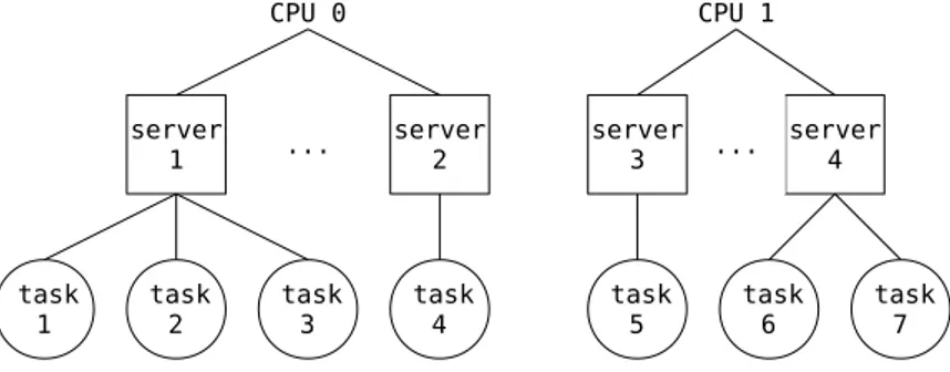
The MRS[9] is a technology developed in Mälardalen Real-Time Research Centre. Its purpose is to enable predictable execution of real-time tasks in multi-core platforms, by regulating the access of shared resources such as CPU and memory. The foundations of MRS is a hierarchical scheduler that allows the user to group tasks into subsystems (servers), and assign limits (budgets) on CPU-time and memory bandwidth. A subsystem can be seen as an autonomous unit that schedules the underlying tasks isolated from the other subsystems. Each CPU core executes a number of subsystems according to a global scheduling policy. ... CPU 0 server 1 task 2 task 1 task 3 CPU 1 server 4 task 7 task 6 ... task 5 server 2 task 4 server 3

Figure 2.1: Visualization of MRS hierarchical structure.

A server is defined by four properties: a priority Ps, a period Ts, a CPU budget Qs, and a memory budget Ms. Similarly a task is defined by a priority Pi, period Ti, a WCET Ci, and deadline Di. A global scheduler on each core is managing the servers. In the beginning of each server period, both CPU and memory budgets are replenished. A

(18)

server then is in the READY state. At every decision point, the global scheduler selects for execution the highest priority READY server. The executing server then locally schedules its tasks. On every system tick the CPU budget is decremented, even if there is no task available for execution (idling server architecture). The memory budget on the other hand, decrements only on a memory request, and it is maintained during the period (deferrable server architecture). If any of the budget is depleted, the server halts execution and transitions to the SUSPENDED state.

2.5 Related work

Contention of the cache is an important problem for the academia and the industry, therefore it has been studied extensively. One of the first studies of the relationship between virtual memory and cache, is presented in [7], where the author examines the effects of different system parameters and page allocation strategies on the cache miss rate. In [13] a compiler-based technique is demonstrated, aiming to reduce cache misses by using a combination of techniques like automatic loop-unrolling, padding and insertion of prefetching instructions.

In [12] the author presents an OS-controlled application-transparent cache-partitioning technique, that leverages the fact that different physical pages fall into different cache lines, a method known as as page coloring. A technique similar to page coloring, is column caching [14]. The idea is to assign tasks in different cache ways or "columns", instead of different sets. In [8], the author used this technique and demonstrated energy savings of up 35% by switching off unused partitions of the cache. Unlike page coloring, column caching requires special hardware. In [15] an adaptive framework is presented, that uses cache partitioning to guarantee QoS for applications with heterogeneous mem-ory access requirements. For [16], absolute performance is not as critical as fair access of the cache for all system tasks. [11] presented a study of the effects of different techniques (static, dynamic partitioning, etc.) in different metrics like QoS and fairness.

(19)

One of their finding is that even though cache partitioning minimizes execution variance, at the same time it can cause increased execution times. [17] is trying to reduce the negative effects of page coloring (waste of memory space), by coloring only a small portion of frequently accessed pages, but reaches the conclusion that additional hardware support is needed for this technique to be practical.

(20)

Chapter 3

Overview of Memory management

in the Linux kernel

Memory in Linux is divided in addresses that point to individual bytes (byte-addressable memory). A n-bit address can point up to 2n different locations; from 0 to 2n− 1. Therefore a 32-bit address space is 4294967296 bytes or 4GiB. Even though each byte is individually addressed, memory is usually manipulated in units called pages. Each page is commonly 4096 bytes long, therefore a 32-bit address space contains 4GiB_4KiB = 1048576 pages. Each address can be divided in two parts; the Page Frame Number (PFN) and the page offset [6].

31 ... 24 23 22 21 20 19 18 17 16 15 14 13 12 11 ... 4 3 2 1 0 Page Oﬀset Page Number 1 1 0 1 0 ... 0 0 0 0 0 0 0 0 0 0 0 0 0 0 ... 0

Figure 3.1: Example of memory address.

3.1 Physical memory

Linux is available for a wide range of platforms, therefore an architecture-independent way to describe physical memory has been implemented. On the highest level, physical

(21)

memory is separated into "nodes". Each memory node is separated into “zones”, and each zone is represented by a struct that points to the equivalent region of a global mem_map array that contains all the pages of that node.

0 MiB (0) 16 MiB (4096) 896 MiB (229376) 4096 MiB (1048575) DMA node

ZONE_DMA ZONE_NORMAL ZONE_HIGHMEM

NORMAL HIGHMEM

mem_map

Figure 3.2: Physical memory zones in x86 Linux[6].

Each zone has different properties. ZONE_DMA is used by certain devices. ZONE_NORMAL is directly mapped by the Kernel. ZONE_HIGHMEM is the rest of the memory.

3.2 Virtual memory

Modern operating systems hide the physical memory from programs through an abstrac-tion called virtual memory. The idea behind virtual memory is that each program should be limited to act within its own private Virtual Address Space (VAS). The VAS of a pro-cess doesn’t directly correspond to any physical memory. Behind the scenes the Kernel is mapping the virtual pages to physical pages as and when needed, and keeps track of the mapping in special tables. Consequently, programs are oblivious not only of other VAS, but also of the physical memory itself.

(22)

rest is reserved for Kernel operations (Kernel space). The proportion between User and Kernel space usually is 3GiB/1GiB, but can be configured during Kernel compilation. The Kernel space portion in every VAS is mapped to the same physical memory.

0x00000000 0xc0000000 User space 3 GB 0xffffffff Kernel space 1 GB Virtual address space of a process

Figure 3.3: User / Kernel space split [6].

The operating system keeps track of the current mapping between virtual pages and physical frames, by using a "page table" structure.

3.3 The buddy system

An efficient operating system must serve memory requests as quickly and efficient as pos-sible. Linux address this issue by using what is know as the buddy system, a mechanism that keeps track of free physical blocks. In each memory zone there is an array defined as:

struct free_area free_area[MAX_ORDER]

Each position of this array represents an incremental "order" from 0 to MAX_ORDER (currently equals to 11). The elements of this array are the HEAD nodes of a linked list. Each of those lists contain free blocks of memory of size 2order, therefore order 0 contains blocks of 20 pages, order 1 contains blocks of 21 pages, up to blocks of 211pages for MAX_ORDER.

When an allocation of a 2n sized block is requested, the allocator simply returns a block from the order n list. In case that there are no free blocks of the requested size, the

(23)

0 1 2 10 MAX_ORDER ... ... ... ... ... ... orders

Figure 3.4: Free block lists in each memory zone [6].

allocator will break up a higher order block into two buddies. This process can continue recursively until the needed sized block is available. The broken buddies are inserted into the lists of the appropriate order.

0 1 2 2 0 1 ... ... a) b) allocate

Figure 3.5: Buddies before (a) and after (b) allocation [6].

The technique is better explained with an example. Assume at some point the system free lists (of some zone) are similar to figure 3.5(a). A request for a single page block arrives but the order 0 free list is empty. Then the buddy system check the next order for a free block but it is also empty. Finally, it checks the next order (order 2), where a free block is available. It removes the block from order 2 and splits it up in two buddies; one is inserted in order 1 and the other is broken up again in two new buddies. One is inserted in order 0 free list, while the other is returned to satisfy the request 3.5(b).

(24)

freed block is available, and if it is, it merge them together creating a single block of higher order, and move it to the higher order list. Then if the higher order buddy is available the same process repeats.

(25)

Chapter 4

Overview of CPU caches

Modern CPU architectures include multiple layers of cache, which is a small, high-speed, low latency memory that resides in or nearby the CPU. By having needed data locally, costly operations to the main memory are minimized. The need for such memory sprang from the fact that CPUs have advanced much faster than RAM, resulting to a perfor-mance gap between the two [5]. In fact, the addition of cache layers is one of the greatest breakthroughs in computer technology.

CPU caches is usually made of Static RAM (SRAM) modules, a very fast type of memory. But why not just manufacture the main memory from SRAM and skip caches altogether? The reason is that SRAM is very expensive and less dense, therefore Dynamic RAM (DRAM) is used instead. DRAM is much cheaper, but at same time much slower compared to SRAM.

The principle of caching consists of keeping a subset of the most frequently needed data locally. Current COTS systems have only a few megabytes of cache but gigabytes of main memory. How is it possible such a small memory to offer any significant benefits? The efficiency of CPU caches comes from the property of locality of reference. It has been observed that when a data location is referenced then it is highly probable that the same location or a related location will be referenced again in the near future. The locality of reference is better illustrated with an example:

(26)

#define SIZE 1000

int i;

int a[SIZE] = {0, 1, 2, 3, 4, 5, 6, 7, 8, 9, ... 999};

for(i = 0; i < SIZE; i++) { a[i]++;

}

As it can be seen, variable i is accessed multiple times in each loop therefore it displays the principle of temporal locality. At the same time, nearby elements of array a[] are accessed sequentially, displaying the principle of spatial locality. Cache memories have evolved to take advantage of both temporal and spatial locality. Therefore just by having a very small portion of the executing program in the cache, a tremendous execution speedup is achieved.

4.1 Address translation and TLBs

System processes are operating on virtual addresses. As a consequence, when an instruc-tion is executed in the CPU, the virtual addresses have to be translated into physical ones, in order to access the right RAM location. The mapping between virtual to physical addresses is kept in the OS page tables, and it would be extremely slow to search through them on every instruction. To avoid this problem, special hardware called Translation Lookaside Buffer (TLB) exist in the CPU, to keep track of the mapping of frequently accessed addresses. As a matter of fact, TLB can be seen as the first caching layer, but it differs from the rest of the caches in that it is caching address mappings and not RAM contents.

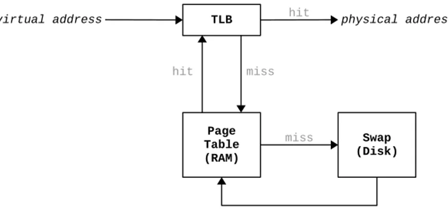
A simplified virtual to physical address translation is illustrated in figure 4.1. When the CPU requests a virtual address translation, the first step is to search in the TLB. In case of a TLB hit the physical address is immediately returned to the CPU. If the requested mapping cannot be located in the TLB, a TLB miss occurs and the mapping

(27)

has to be fetched from the page tables (which reside in RAM). If swapping is enabled it is possible to have a page table miss because the requested page is swapped out to the hard disk. In that case it has to moved into RAM and assigned a physical address. After the page is located in the page tables, the mapping is written to the TLB and the stalled instruction can be re-executed.

TLB

virtual address hit physical address

Page Table (RAM) Swap (Disk) miss miss hit

Figure 4.1: Virtual to physical address translation.

4.2 Instructions and data caching

After the physical address of a data location is resolved, a new RAM request generated to read or write the contents of that location. Therefore the usual CPU - RAM bottleneck appears again, but fortunately caches are used again to minimize its effects. Modern designs carry not one but multiple levels of caches (and TLBs), commonly referred as L1, L2, ..., Ln. Each cache layer towards RAM has the property of being larger and but slower than the previous one. Additionally, most architectures are using separate caches for data and instructions (at least for some layers), to achieve increased performance by resolving and fetching instructions and data simultaneously. For example, the cache hierarchy of the CPU used in this project, can be seen in figure 4.2 (data provided from CPUWorld[2]).

In order to take advantage of spatial locality whole chunks of data is fetched and cached during a cache miss. This chunk is called cache line and commonly is 64 bytes

(28)

TLB 0 data TLB 1 data TLB instruct. TLB 2 unified L1 data L1 instruct. L2 unified L3 Core 0 Core 1 Core 2 Core 3

Figure 4.2: Intel i5 3550 TLB and cache layers.

long. The cache line contains both the requested location as well as nearby ones, and is calculated as following:

line size = 2b bytes line offset = b

line memory address = bmemory address

line size c, 1 ≤ line size ≤ 2

31

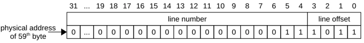
For example if line size = 24, the 59th byte of memory is contained by line number 3 because:

line offset = 4

line memory address = b59 24c = 3

The same observation can be made on a binary level:

31 ... 19 18 17 16 15 14 13 12 11 10 9 8 7 6 5 4 3 2 1 0 line offset line number 1 1 0 1 0 ... 0 0 0 0 0 0 0 0 0 0 0 0 0 0 1 1 physical address of 59th_byte

Figure 4.3: Line number and offset of an address.

The offset is represented by the lowest log₂(line size) bits of the address, and the line number by the following bits. Note that the line number refers to the location of the line in physical memory. The line location in the cache will be analyzed in the following

(29)

sections. This mapping is very important, because the it has to be fast and at the same time utilize the available cache space in an effective manner. These two goals are contradicting (at least for current technology), therefore different mapping techniques have been proposed to address different goals. Three of the most common types are fully associative, directly mapped and set associative.

4.2.1 Fully associative cache

It is perhaps, the most straightforward way of caching data. The cache can be imagined as an array of lines. When a memory line must be cached, it can be placed anywhere, according to some replacement policy (commonly LRU). When the CPU requests some data, the whole cache must be searched sequentially in order to locate a line (or determine that it is not in the cache). This scheme provides very effective space utilization and minimize collisions for frequently needed data, but on the other hand, sequential search can be very slow.

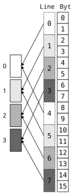
4.2.2 Directly mapped cache

The opposite of a fully associative cache is the directly mapped cache. It is still an array of lines, but each line to be cached is mapped strictly to one and only one location or index, depending on its location in physical memory (line memory address).

cache index = line memory address MODULO cache size, (cache size counted in lines)

The benefit of this cache is speed since the location of requested data is deterministic. At the same time, the speed comes at the cost of bad space utilization: colliding lines are evicting each other even though there might be plenty of locations (of less needed data) that they can go.

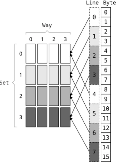
4.2.3 Set associative cache

A set associative cache is an attempt to combine the benefits of the other two types. This time the cache is a two-dimensional array, where each line of the array is called

(30)

0 1 2 3 Byte Line 0 1 5 2 6 7 3 4 0 1 2 3 4 5 6 7 8 9 10 11 12 13 14 15

Figure 4.4: Example of a directly mapped cache of 4 lines, with line size of 2 bytes). Gray colors are used to highlight the memory - cache mapping. Note how addresses with the same color fall in the same cache line.

"set" and each column is called "way". The memory line can go to one and only one set, determined in a similar fashion as the directly mapped cache. Inside the set though, it can go to any way , in the same manner as a fully associative cache. Directly mapped and fully associative caches can be seen as extreme cases of a set-associative cache: a set associative cache with s sets and 1 way behaves like a directly mapped cache, whereas one with 1 set and w ways behave like a fully associative cache.

A cache address has three parts; the tag, the set index, and the offset. The particular characteristics of the cache must be known, to determine the mapping of the data. The cache size and associativity are usually available for a given architecture, and from that we can calculate in how many sets are in the cache, and how memory lines are mapped into it.

number of sets = cache size line size ∗ associativity

set index = line memory address MODULO number of sets

(31)

0 0 Way Set 1 2 3 1 2 3 Byte Line 0 1 5 2 6 7 3 4 0 1 2 3 4 5 6 7 8 9 10 11 12 13 14 15

Figure 4.5: Example of a set associative cache of 4 sets x 4 ways, with line size of 2 bytes). Gray colors are used to highlight the memory - cache mapping. Note how addresses with the same color fall in the same cache set.

in the cache.

4.3 Cache Partitioning via Page Coloring

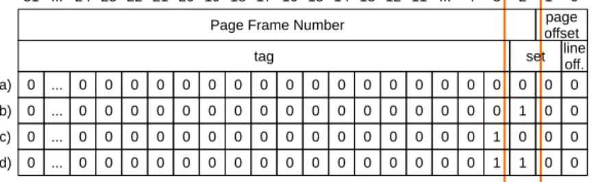
Now that some of the main concepts of caches have been analyzed, it is time to explain how the mapping between virtual and physical memory can be utilized in order to par-tition the cache. Assume a 32-bit system with page-size=4 Bytes and line-size=2 Bytes running on a CPU with a 32 Byte 4-way set associative cache. From this information the following can be derived:

number of sets = 32 2 ∗ 4 = 4 line offset = 1 page offset = 2

By examining the cache set and PFN fields of an address, it can be observed that one bit is overlapping. That means that the PFN can control to some degree in which

(32)

set the particular page lines will fall. This property can be leveraged to achieve cache isolation, a technique known as age coloring. The number of colors/partitions is defined as:

colors = 2set/PFN overlaping bits

31 ... 24 23 22 21 20 19 18 17 16 15 14 13 12 11 ... 4 3 2 1 0 Page Frame Number

0 0 0 0 0 ... 0 0 0 0 0 0 0 0 0 0 0 0 0 0 0 0 page offset

tag set line_off.

0 0 1 0 0 ... 0 0 0 0 0 0 0 0 0 0 0 0 0 0 0 0 0 0 0 1 0 ... 0 0 0 0 0 0 0 0 0 0 0 0 0 0 0 0 0 0 1 1 0 ... 0 0 0 0 0 0 0 0 0 0 0 0 0 0 0 0 a) b) c) d)

Figure 4.6: Page coloring: overlapping set and page bits.

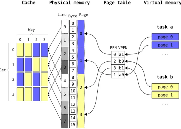
Now assume that in the system there are two tasks running: a and b. Depending on the particular execution, task might be mapped to PFN 0 and 1 and task b to 2 and 3. As it can be seen in figure 4.7, this random mapping makes tasks to compete for the same cache space.

This situation can be prevented through page coloring. The number of colors is colors = 21 = 2 so the cache can be divided in two partitions. By mapping the pages with color 0 to task a and pages with color 1 to task b, cache isolation can be achieved. It should be mentioned that page coloring is applicable only for single-page requests (order 0), because the LSB that determines the color of a page, matches with the LSB of the PFN. Therefore, consecutive PFNs have different colors and as a result, higher-than-zero order blocks, contain multiple colors.

(33)

0 1 2 3 VPFN PFN 0 0 Set 1 2 3 1 2 3 Byte Line Page Physical memory task a a1 b0 b1 a0 0 2 3 1 Way page 0 ... page 1 task b page 0 ... page 1 0 1 2 3 4 5 6 7 8 9 10 11 12 13 14 15 Virtual memory Page table Cache 0 1 5 2 6 7 3 4

(34)

0 1 2 3 VPFN PFN 0 0 Set 1 2 3 1 2 3 Byte Line Page Physical memory task a a1 b0 b1 a0 0 3 1 2 Way page 0 ... page 1 task b page 0 ... page 1 0 1 2 3 4 5 6 7 8 9 10 11 12 13 14 15 Virtual memory Page table Cache 0 1 5 2 6 7 3 4

Figure 4.8: Page coloring allocation: Through careful virtual-to-physical page mapping, task a and task b end up in different cache sets, thus they are isolated from each other.

(35)

Chapter 5

Design and Implementation

page_alloc.h page_alloc.c coloring.h coloring.c Kconﬁg mmzone.h api.h resch.c memsched.c libresch.a

Kernel-space

User-space

task ioct l() PGC Conﬁguration PGC Allocator PGC Control Modules API deﬁnitions Call library

Page coloring was implemented by modifying the buddy system as following: Instead of returning the first free page, the buddy system lists are searched in order to locate a page of the correct color. If such a page is not found in order 0, higher order blocks are broken into single pages, similarly to the original buddy system. Pages that are not matching the requested color, are not inserted back into order 0, but instead are separated into indexes(lists). As long as the index of the appropriate color is not empty,

(36)

a request of that color can be satisfied immediately, without having to search the buddy lists. This process can be seen in flowchart 5.1.

Request for page of color C

index of C is empty

Return first page from index[C] Request failed No Ye s order < MAX_ORDER order = 0 order has free blocks

Remove block from order. Insert block page(s) into indexes

Ye s No order += 1 Ye s No index[C] is empty Yes N o

Figure 5.1: Flowchart of color-aware physical memory allocator.

This technique was presented in PALLOC[10] project paper. As it will be explained in the rest of the chapter, the current implementation differentiate in tree main points:

• A different method is used to extract the color of a page.

• Freed pages are re-inserted into the appropriate color index, instead of returning them to the buddy system lists.

(37)

• The current work utilize the fork-exec technique to color a process, PALLOC is using cgroups.

5.1 PGC configuration

One important consideration was how to configure and specify system-specific parame-ters, regarding page coloring. To keep track of the address bits that define the color of a page, two parameters were specified in /include/linux/mmzone.h. The first is PGC_MASK_LEN which defines the number of bits to be used for coloring, and the second is PGC_LSB that specifies the least significant bit of that range. PGC_LSB is equal with the PAGE_SHIFT, while PGC_MASK_LEN is equal with 1...i, where i is the number of overlapping PFN and Set index bits, and can be specified during Kernel configuration. Based on these values, two more parameters were specified as a "shortcut" for common operations. The first is PGC_SYS_COLOR_MAX which represents the maximum number of colors the system can have, and PGC_MASK which is a bit mask of 1’s that will be used to extract the color of a page with bit-wise operations.

... PGC_LSB = PAGE_SHIFT PGC_MASK_LEN = 1...i PGC_SYS_COLOR_MAX = 1 << PGC_MASK_LEN PGC_MASK = PGC_SYS_COLOR_MAX - 1 ...

In the same file, an array of lists was added to the zone struct, that will be used to index pages according to their color.

...

struct zone {

/* Fields commonly accessed by the page allocator */ struct list_head pgc_index[PGC_SYS_COLOR_MAX]; ...

(38)

} ...

The system configuration is made from a kernel configuration utility, menuconfig for example. The user can specify the following parameters:

• Enable/Disable page coloring.

• Select CPU profile.

• Select number of colors.

• Enable/Disable page coloring related debugging.

Figure 5.2: Page coloring Kernel properties.

5.2 PGC control

(39)

• Start/Stop page coloring.

• Set the color for the currently executing process.

• Show processes of a specific color.

• Flush indexed pages.

The parameters and functions that control the PGC allocator were declared and spec-ified in include/linux/coloring.h and mm/coloring.c. Additional implementation details can be found in appendix C.

5.3 PGC allocator

The "business" function of the buddy system is __rmqueue_smallest in mm/page_alloc.c. A modified version of this function, along with pgc_index_insert, *pgc_index_extract, pgc_index_flush, compose the PGC allocator system, as specified in figure 5.1. More implementation details can be found in appendix C.

To expose some internals of page_alloc.c, and in particular to be able to flush the color indexes from the userspace, a header file for mm/page_alloc.c was added to the system (/include/linux/page_alloc.h).

void pgc_index_flush(struct zone *zone);

5.4 Userspace - Kernelspace communication

Different communication methods were considered such as procfs, sysfs, signals, and socket based mechanisms, but ultimately ioctl calls were used, as per the MRS implemen-tation. To access page coloring related functions from the userspace, the following API calls were defined in MemSched/core/api.h and additional cases were added in resch.c to serve them.

(40)

ioctl call Service routine API_PGC_STATE pgc_set_state() API_PGC_SET_CURR_C pgc_set_current_c() API_PRINT_PROC pgc_print_c_proc() API_INDEX_FLUSH pgc_flush_indexes()

Table 5.1: Page coloring API

5.5 How a color is assigned to a process

One of the main components of page coloring is the mechanism of assigning a color to a process. Such a mechanism should work at/before the process creation, otherwise the process would be uncolored for sometime, and it might request memory of the wrong color. Additionally, this mechanism should operate at a sufficiently low level so that the memory allocator can be aware of it.

In Linux, new processes are created by a technique known as fork-exec. The fork() system call splits an existing process into two identical processes, by creating a new task_struct that has the same parameters as the original one. The exec() system call is then used to switch one of the processes, usually the new one, to a different context. Obviously, a "first" process is needed from which all the other processes will spawn. In Linux this process is called init. The init process serves one more purpose: A parent process might finish execution before a spawned child process. In this case the child task will become a "zombie" process, as there is no one to collect its SIGCHLD status signal. To prevent this problem, init automatically adopts the orphaned processes.

With some modifications, the fork-exec technique can be easily utilized to color to a task. A color property must be added to the Linux task_struct structure (/include/lin-ux/sched.h). In the current work, it was decided that each process will have one and only one color, therefore a simple integer is enough to represent it.

struct task_struct { unsigned int color;

(41)

... }

During the fork() system call, when the copy_process() is called, copy the parent color to the child along with the other properties.

/*

* This creates a new process as a copy of the old one, * but does not actually start it yet.

*

* It copies the registers, and all the appropriate * parts of the process environment (as per the clone * flags). The actual kick-off is left to the caller. */

static struct task_struct *copy_process(...) {

...

p->color = current->color; ...

}

In figure 5.3, it can be seen how to color and execute process tsk in color 2: First a parent process starts execution and change its current color with an ioctl call. Then a fork() call is used to spawn a child process that will inherit all the properties including the color. The parent process then exits, while the child process calls exec() to switch to tsk context.

All processes default to color 0. That means that the other colors are free and can be used to isolate the target tasks. We found that this method offers the best isolation. On the other hand, if the system is divided by too many colors, each color will have very little main memory, and as a result system tasks might crash. We found that a computer with 4 GiB of RAM was stable with up to eight colors but large applications (eg. firefox) had to be assigned exclusively in separate colors. Note that isolated processes can still

(42)

fork() color 0 parent _color(2) color 2 parent color 2 parent color 2 child exit() exec() color 2 tsk end

Figure 5.3: Coloring of a task using fork-exec.

pollute each other indirectly. If one of those tasks performs a kernel call, the kernel call might compete with tasks of other colors.

To simplify the coloring of a process, and at the same time allow legacy processes to be colored, a special utility called exec-colored, was developed. To give an example of its use, if the user wants to start a process called tsk in color 2, the following command can be given in the command line:

exec-colored 2 tsk

5.6 Integration with MRS

The color-aware allocator mechanism is enabled in the Kernel itself, and therefore, apart from modifying resch module to accept the new PGC API, no other integration is needed. It is enough to color the tasks in start.sh using the exec-colored tool. We nevertheless noticed some problems. According to the requirements, the cache partitioning should be done per server, and all the tasks of the said server should execute in that cache partition. Under the current configuration process, it is very difficult to do so. Moreover, manual configuration of MRS is elaborate and error prone, since cores, servers and tasks are initialized from different locations; the number of cores is defined in Resch configure file, the server properties are set with preprocessor #define commands in MRS module, and task properties are passed from the command line (start.sh). To address these two problems, a simple front-end / configuration tool, was implemented.

(43)

The first part of the front-end is an input file encoded in JSON, a human-readable data exchange format that is very easy to use. In the beginning of the file, the user declares the global system parameters, like load balance or maximum number of tasks (as per Resch configure file). Then she declares a "cores" list which contains an entry for each core that will be active for the simulation. The cores should be declared incrementally; the first entry represents core 0, the next core 1, etc. Each core entry contains a "servers" list which contains the information for each server that is to be run on that core. Similarly, each server entry contains a "tasks" list that contains information regarding tasks that will be run on that server. The second part is a parser written in Perl, that decodes the input file and automatically extracts and configures all the parameters that previously had to be meticulously specified in different files. To give an example, a system with one core running a server that contains two tasks might be:

{ "loadbalance":"0", "maxrttasks":"64", "cores":[ { "servers":[ {

"id":"0", "priority":"0", "period":"60", "cpubudget":"8", "

,→ membudget":"750", "color":"1", "tasks":[

{ "priority":"99", "period":"300", "wcet":"1", "name":"RT", "

,→ exec":"./test/task1" },

{ "priority":"98", "period":"20", "wcet":"5", "name":"normal",

,→ "exec":"./test/task2" } ] } ] } ]

(44)

}

This system can open new opportunities for future work. For example it makes it very easy to create a GUI front-end for MRS, or receive input from a simulation tool.

JSON input file Perl parser

b) User servers sample.sh memsched.c a) User start.sh resch/configure tasks servers sample.sh memsched.c start.sh resch/configure tasks

(45)

Chapter 6

Results

6.1 Evaluation setup

All the experiments were performed on a quad core Intel Core i5-3550 CPU, with a shared 6MiB L3 LLC. The system memory was 4GiB. The OS was Ubuntu 12.04 LTS, with linux-3.6.11.9-rt42 Kernel, which was compiled as explained in appendix A. The experiments were run on the command line, outside of any graphical environments, in order to minimize interference caused by unrelated tasks.

6.2 Tests and benchmarks

6.2.1 Test 1: Coloring of a task

The goal of this test is to prove the correctness of the coloring mechanism. A firefox instance was used as a target task, and was mapped to color 3 with the exec-colored utility. Then the show_c_proc utility was run, to show which tasks are assgned to color 3:

exec-colored 3 firefox ./build/show_c_proc 3 dmsg

(46)

6.2.2 Test 2: Correctness of color-aware allocator

The aim of this test is to verify that tasks are allocated into pages of the assigned color. Linux provides two files from which the physical mapping of each task can be extracted; /proc/pid/maps that contains the virtual pages in use, and /proc/pid/pagemap that con-tains the mapping between virtual and physical pages. To read those files, a customized version of the open source tool page-collect [3] that was used. This tool is accepting as input arguments the color LSB, the color mask length, and the process id. The output is a file that contains the physical memory mappings.

page-collect 12 2 $(pidof firefox) ... /usr/lib/firefox/firefox: 0...000000001101111010110011|11|000000000000 /usr/lib/firefox/firefox: 0...000000001101111010110100|11|000000000000 /usr/lib/firefox/firefox: 0...000000001101111010110101|11|000000000000 /usr/lib/firefox/firefox: 0...000000001101111010111001|11|000000000000 ...

The bits that define the color of each page are highlighted between the pipe characters (| |). It can be seen that all the pages are of color 2 (11 in binary). For comparison, if the test is repeated under a default memory mapping policy, the task instance is allocated in pages of all colors.

page-collect 12 2 $(pidof firefox) ... /usr/lib/firefox/firefox: 0...000000101100010000101011|11|000000000000 /usr/lib/firefox/firefox: 0...000000101100010000101100|00|000000000000 /usr/lib/firefox/firefox: 0...000000101100010000101100|01|000000000000 /usr/lib/firefox/firefox: 0...000000101100010000101100|10|000000000000 ...

(47)

6.2.3 Experiment 1: Behavior of single task

In this experiment the goal is to determine the relationship between cache misses, task data size and cache partition size. A special task called arrayloop was developed and used as a workload for this experiment. This task would first allocate and then randomly access a data array of a given size. The arrayloop task is executed using seven different data sizes: 0.5MiB, 1MiB, 1.5MiB, 2MiB, 4MiB, 6MiB, 8MiB. Each instance was executed under four different cache sizes/scenarios: (A) Each task instance is executed without cache partitioning, sharing the whole cache (6MiB) with the Kernel. (B) The cache is divided into two 3MiB partitions; partition 0 is assigned for the Kernel, and partition 1 to the task instance. (C) The cache is divided into four 1.5MiB partitions. Again, partition 0 is reserved for the kernel and partition 1 for the task instance. (D) The cache is divided in eight partitions of 0.75MiB. The Kernel and task instance are isolated in the same way as the previous scenarios. Each task instance was executed one by one, aiming to determine its performance without interference. The results were collected using the perf tool[4], that monitors the CPU performance counters.

Array size

0.5 MiB (t1) 1.0 MiB (t2) 1.5 MiB (t3) 2.0 MiB (t4) 4.0 MiB (t5) 6.0 MiB (t6) 8.0 MiB (t7)

Cac he si ze 0 0 0 0 1.04 12.17 30.67 0 0 0 0 28.87 52.04 63.21 1.5 MiB (C) 0 0 4.33 29.06 63.9 74.24 78.78 0 28.86 53.24 65.21 81.1 85.01 85.62 6 MiB (A) 3 MiB (B) 0.75 MiB (D)

(48)

6 MiB (A)0 3 MiB (B) 1.5 MiB (C) 0.75 MiB (D) 10 20 30 40 50 60 70 80 90 0.5 MiB (t1) 1.0 MiB (t2) 1.5 MiB (t3) 2.0 MiB (t4) 4.0 MiB (t5) 6.0 MiB (t6) 8.0 MiB (t7) Cache Size C ach e mi ss es %

Figure 6.2: Experiment 1 - Plot of cache misses vs cache partition size.

6.2.4 Experiment 2: Isolation of parallelly executing tasks

The aim of this experiment is to investigate the behavior of parallelly executing tasks, how they affect each other, and to verify that page coloring is indeed minimizing interference of the L3 cache.

In the first scenario (E) of this experiment, scenario (A) is repeated with one dif-ference: the seven arrayloop task instances are executed concurrently. In the second scenario (F), the same task set is used again, but this time each instance is isolated in a different color/partition of 0.75MB. The Kernel is again isolated in its own partition.

(49)

Array size C a ch e Si ze _1.52 _3.84 _16.22 _38.17 _74.67 _82.08 _87.8 0.18 28.75 53.02 64.65 80.18 83.32 83.51 0.5 MiB

(t1) 1 MiB(t2) 1.5 MiB(t3) 2 MiB(t4) 4 MiB(t5) 6 MiB(t6) 8 MiB(t7)

6 MiB (E) 0.75 MiB

(F)

Figure 6.3: Experiment 2 - Results.

(A) (E) (D) (F) 0 10 20 30 40 50 60 70 80 90 100 t1 t2 t3 t4 t5 t6 t7 Cach e misses %

Figure 6.4: Experiment 2 - Plot of cache misses in each scenario.

6.2.5 Experiment 3: MemSched with cache partitioning

In the first scenario (G) of the experiment, a single server with a single task is created in order to benchmark the performance when running alone in the whole cache. The task used is a modified version of arrayloop that benchmarks and prints the execution time of each period.

In the second scenario (H), a second server with a memory demanding task is added to the system. The servers are allocated in different CPU cores to run concurrently. The server and task properties can be seen in tables 6.1 and 6.2.

(50)

Server Core Priority Period CPU-budget Mem-budget

0 0 0 60 8 750

1 1 0 5 1 750

Table 6.1: Experiment 3: Server configuration

Task Server Priority Period WCET Size (MiB)

RT 0 99 300 1 0.5

MEM 1 99 15 1 5

Table 6.2: Experiment 3: Task configuration

Scenario Execution time (ms)

RT (G) 10.57

RT + MEM (H) 127.19

RT + MEM, isolated (I) 12.8 Table 6.3: Experiment 3: Results

In the third scenario (I), the cache is separated in four colors of 1.5MiB, and each server is allocated to a different color. The results of experiment 3 can be seen in table 6.3. Similarly to previous experiments, the kernel is isolated to color 0 so as it is not interfering with the servers.

6.2.6 Experiment 4: Overhead of PGC allocator

To measure the overhead of the custom allocator, a "before" and "after" nanosecond-precision, per-CPU timestamps were added to the buffered_rmqueue function. Experi-ment 2 was re-run first on the default and then on the PGC kernel. The collected results can be seen in figure 6.4.

(51)

Default Kernel PGC Kernel

Min (ns) 49 68

Max (ns) 11734 14898

Avg (ns) 211 325

(52)

Chapter 7

Discussion

The strategy behind the experiments was to build confidence incrementally; first by testing the simpler aspects of the system and them move towards the more complex experiments.

Beginning with Test 1, it was verified that the fork-exec technique is working correctly, and a task can be colored to the desired color. Test 2 verified that tasks are allocated only into physical pages of the correct color - with an exception: Shared libraries are allocated to color 0 pages by default.

In Experiment 1, the goal was to determine the relationship between cache misses, task data size and cache partition size. The initial results were mixed and for this reason many different workloads were used. At some point it was realized that the CPU prefetching of instructions and data into the caches is distorting the measurements. Prefetching can sometimes be disabled through the BIOS or by setting special registers, but neither option was available on the given hardware. This was discovered late in the thesis, and there was no alternative hardware available.

As a workaround, the arrayloop utility was designed to use random reads to neutralize prefetching. Assuming perfectly isolated cache partitions and random reads, the cache miss rate is directly related to the amount of data the cache partition can hold:

(53)

miss rate =     

0, if data size ≤ partition size

data size−partition size

data size ∗ 100, otherwise

(7.1)

The measured results of scenarios (A),(B),(C),(D) are matching very closely the expected model. For example, in case of a 4MiB arrayloop task allocated in a 0.75MiB partition, the expected value of cache misses is 4−0.75₄ ∗ 100 = 81.25%, and the measured is 81.10%, for 8Mib arrayloop task in a 3MiB partition the expected value is 8−3₈ ∗ 100 = 62.5% and the measured is 63.21%, and similarly for the rest of the measurements. These results show that the page coloring mechanism has indeed partitioned the cache.

The next step was to establish if task isolation has been achieved. In scenario (E) of Experiment 2, the task set of scenario (A) was rerun, but this time all the tasks were run concurrently. As a result, the cache misses have greatly increased. This is expected, since multiple tasks are competing for the same cache space (and the cache can’t fit everything). Another observation is that larger tasks seem to be more affected than the small ones. This is explained considering the L3 cache LRU replacement policy: By the time the 8MiB task gets to read all of its elements (a single time), the 2MiB task has read them four times. Each time an element is read, the equivalent cache line flags are refreshed and that makes cache lines of the smaller tasks to be "fresher". On the contrary, the larger task cache lines are more "stale" and more likely to be replaced. In scenario (F) the picture is different. It can be seen that the cache misses of the smaller tasks have increased (data can’t fit in the smaller space and cause self eviction). The misses of the larger tasks though, have been slightly decreased because the competition from the small tasks have been eliminated. Comparing the results of scenario (F) with scenario (D), we can observe very good isolation.

In Experiment 3, page coloring and MemSched were put together, something that is one of the main objectives of the thesis. In scenario (H) the RT task is highly affected by the memory intensive task MEM. In scenario (I) the servers are assigned into different cache partitions, and the execution time of the RT task is greatly improved due to cache

(54)

isolation.

In the last experiment, the overhead of the PGC allocator was measured and com-pared to the default linux kernel. The custom allocator is slower that the default one, something that was expected. The default kernel serves some of the memory requests from private per-cpu structs, whereas in the PGC kernel all memory requests are served from the zone lists (buddy or color index), something that demands the acquisition of a global lock in every allocation. In feature work, it might be possible to distribute the color indexes as per-cpu structs, in order to avoid this problem.

(55)

Chapter 8

Conclusion

Based on the collected results, we believe that the objectives of this project were met. From a raw performance point of view it is difficult to beat modern large, highly associa-tive caches, but from a real-time systems perspecassocia-tive our results show a tangible benefit of isolating servers and tasks into different memory partitions.

8.1 Future work

There are numerous ways the research can be continued. First, the performance of the colored memory allocator can be improved. According to the current design the per-CPU free pages have been disabled and every memory request is forwarded to the buddy system. This is something costly because the global memory zone lock has be locked, possibly affecting the other cores. If a per-CPU color index is implemented, it will be possible to serve a memory request immediately, and resort to the buddy system only when no pages of the right color exist in the per-CPU index. A per-CPU color index can lead to interesting possibilities, such as indexing of different colors on different cores.

Another implication of our approach is that only one color can be assigned to each task and as a result the partition size has to remain relatively large. For example our system can support up to 128 cache partitions, but in practice we could’t use more than 8 partitions, because the individual partition size became too small to fit the kernel.

(56)

Mul-tiple colors per task will overcome this problem and allow a more fine-grained control. Also it will allow different optimization objectives; reduce self eviction (allocate consec-utive memory allocation requests to different colors) or reduce interprocess eviction (as we did in this work) or both.

One more idea is to impose a quota on the color indexes. We noticed that the current indexing algorithm was too aggressive and break down most of the physical memory into single page blocks. That can make requests for larger-than-one-page memory blocks, to fail. We found our implementation to be very stable, but having a quota will make the allocator able to respond well in all workloads, and therefore even more robust.

We also found that MRS project is becoming more and more complicated. It was initially build as an extension to the Resch project that was promoted as a platform independent scheduling framework. The later additions of multi-core capabilities and memory throttling needed special kernel compilation options and rendered the benefit of platform independence less relevant. Cache partitioning is completely depended on custom kernel and therefore it might be beneficial to convert MRS into a standalone project that will be less complex, more stable and better performing. We also believe it is time to shift to a 64-bit architecture, the current standard for COTS systems.

Furthermore, using the current work as a basis research can continue to new di-rections. A natural step ahead is Memory Bank partitioning; allocate different tasks to different memory banks in order to bound RAM response time on a hardware level. Even though this idea has already been investigated by the academia, we believe that it will be interesting to combine it with with the current and previous work, creating a holistic approach that could offer tighter real-time guarantees to COTS hardware.

(57)

Appendix A

Installing the RT Kernel

A.1 Introduction

This guide explains how to download, patch, compile and install the RT Linux kernel. The version used in this project is 3.6.11.9, but the same steps should be applicable to other 3.x versions. More details can be found at Real-Time Linux project FAQ page[1]. Before starting it is a good idea to backup any valuable data (or even better mirror the hard drive).

A.2 Prerequisites

• OS installed: Ubuntu-12.04.4-desktop-i386 (also tested on 10.04).

• Packages installed: build-essential fakeroot libncurses5-dev kernel-package.

• About 10GB of disk space.

• Administrator (root) access to the system.

A.3 Get the source

(58)

mkdir Workspace cd Workspace wget www.kernel.org/pub/linux/kernel/v3.x/linux-3.6.11.tar.xz wget www.kernel.org/pub/linux/kernel/projects/rt/3.6/stable/patch-3.6.11.9.xz wget www.kernel.org/pub/linux/kernel/projects/rt/3.6/patch-3.6.11.9-rt42.patch. ,→ xz tar xf linux-3.6.11.tar.xz mv linux-3.6.11 linux-3.6.11.9-rt42 cd linux-3.6.11.9-rt42 xz -dc ../patch-3.6.11.9.xz | patch -p1 xz -dc ../patch-3.6.11.9-rt42.patch.xz | patch -p1

A.4 Configure

Now it is time to configure the kernel. There are many ways to do so, but perhaps the simplest and most commonly used is the menuconfig utility.

make menuconfig

A graphical display will pop-up where the kernel options can be set. For did the following changes:

General setup

[] Support for paging for anonymous memory (swap)

Processor type and features

Preemption Model --> Preemption Model (Voluntary Kernel Preemption (Desktop) High Memory Support --> 4GB

Timer frequency --> 1000 HZ

Power management and ACPI options

CPU Frequency scaling --> [] CPU Frequency scaling

(59)

A.5 Build

Now the kernel is ready to be compiled. The basic command is:

make deb-pkg

For many-core systems we can speedup the compilation process by using the flag -j to create more threads, usually one per physical core. Instead of specifying a hard coded value, a good trick is to acquire dynamically the number of cores with the command $(getconf _NPROCESSORS_ONLN).

It is worth mentioning that the kernel is compiled with debugging information in-cluded by default (called debugging symbols). These symbols allow the debugger to ac-quire more detailed information on execution, and not just memory addresses. However, the debugging symbols increase the size of the kernel significantly and can be removed, if not needed, by using the flag INSTALL_MOD_STRIP=1.

After putting everything together the compilation command is:

make INSTALL_MOD_STRIP=1 deb-pkg -j$(getconf _NPROCESSORS_ONLN)

The compilation time depends on the hardware and kernel configuration but generally it takes 20 - 60 minutes. Recompilations are much faster, because only the changed files are compiled. Sometimes though, stale object files might conflict and in this case a cleanup is necessary:

make clean

This command removes most of the generated files. There is also the flag mrproper that does what clean does and also removes the configuration files and returns the source to pristine condition:

(60)

A.6 Install

After successful compilation, a few .deb files should exist in the parent folder. To install the new kernel image and headers:

cd ..

sudo dpkg -i linux-headers-3.6.11.9-rt42_3.6.11.9-rt42-X_i386.deb linux-image

,→ -3.6.11.9-rt42_3.6.11.9-rt42-X_i386.deb (Replace X with ./linux

,→ -3.6.11.9-rt42/.version number)

Before rebooting the system, edit the Grub configuration file /etc/default/grub. Comment out the two "HIDDEN" lines as following:

GRUB\_DEFAULT=0

# GRUB_HIDDEN_TIMEOUT=0

# GRUB_HIDDEN_TIMEOUT_QUIET=true GRUB_TIMEOUT=10

This will prevent Ubuntu silently booting the latest kernel version available. For the changes to take effect, update Grub configuration:

sudo update-grub

Reboot the computer and, hopefuly, the new and old kernels should be shown in Grub menu.

A.7 Post configuration

After booting a kernel, it is possible to verify what configuration options have been set, by probing the /boot/config file:

uname -a

cat /boot/config-‘uname -r‘ | grep HZ cat /boot/config-‘uname -r‘ | grep PREEMPT etc...

(61)

Appendix B

Installing the Perf tools

To build the perf tools, we have to manually compile them since we are using a custom kernel.

sudo apt-get install libgtk2.0-dev libdw-dev binutils-dev libnewt-dev bison

,→ flex python-dev

mkdir /build/perf

cd linux-3.6.11.9-rt42-coloring/tools/perf make O=~/build/perf

make O=~/build/perf install PATH=$PATH:~/bin

Sometimes the kernel map address access is restricted, and in that case, the following message is displayed.

perf record -f -- sleep 10

WARNING: Kernel address maps (/proc/{kallsyms,modules}) are restricted, check /proc/sys/kernel/kptr_restrict.

Samples in kernel functions may not be resolved if a suitable vmlinux file is not found in the buildid cache or in the vmlinux path.

(62)

If some relocation was applied (e.g. kexec) symbols may be misresolved even with a suitable vmlinux or kallsyms file.

To fix this problem:

sudo su

echo 0 > /proc/sys/kernel/kptr_restrict

(63)

Appendix C

Implementation Details

C.1 include/linux/coloring.h

#define ULONG_BITS 32

// The purpose of these variables is to be read from the debugfs system. extern const unsigned int pgc_colors;

extern const unsigned int pgc_mask_bits; extern const unsigned int pgc_mask; extern const unsigned int pgc_lsb;

// State of page coloring, 0:OFF, 1:ON extern int pgc_state;

// Running count of indexed pages per color. extern uint32_t index_counter[PGC_SYS_COLOR_MAX];

// Memory requests per order and color.

extern uint64_t mem_req[PGC_SYS_COLOR_MAX][MAX_ORDER];

(64)

void pgc_print_all_c(void);

// Set the color of current process equal to c. int pgc_set_current_c(unsigned long c);

// Enable or disable page coloring according to flag. int pgc_set_state(unsigned long flag);

// Flush indexed pages back to free memory areas. int pgc_flush_indexes(void);

// Print to dmesg tasks per color c. int pgc_print_c_proc(unsigned long c);

// Debug function that converts the UL address n to binary string buffer. void ul_to_bin_string(unsigned long n, int length, char *buffer);

// Debug function that converts UL address n to a binary string buffer // and shows the masked bits according to mask and lsb. buffer must be // of length ULONG_BITS + 3, in order to accomodate the address bits, // the terminating char and the two delimiter chars.

void show_masked_bits(unsigned long n, char *buffer, unsigned long mask, unsigned long lsb);

C.2 mm/page_alloc.c

static inline

struct page *__rmqueue_smallest(struct zone *zone, unsigned int order, int migratetype)

{

unsigned int current_order; struct free_area * area; struct list_head *curr, *tmp;

(65)

struct page *page;

// If page coloring is disabled or requested order is > 0. if (!pgc_state || order > 0) {

goto normal_buddy_alloc; }

page = NULL;

// Try to get a page from the index.

page = pgc_index_extract(zone, current->color); if (page) {

return page; }

// If execution goes here, there was no page in the index.

// Traverse the entire order list 0 - MAX_ORDER.

for (current_order = 0; current_order < MAX_ORDER; ++current_order) { // For each order...

// Check for free memory.

area = &(zone->free_area[current_order]);

if (list_empty(&area->free_list[migratetype])) { // No free blocks in this order.

continue; }

list_for_each_safe(curr, tmp, &area->free_list[migratetype]) { // For each block in free_list...

page = list_entry(curr, struct page, lru); pgc_index_insert(zone, page, current_order); page = pgc_index_extract(zone, current->color);

(66)

if (page) { return page; } } } //else goto normal_buddy_alloc; }

// Break down a block of memory to single pages and place them to the // appropriate index.

static void pgc_index_insert(struct zone *zone, struct page *page, int order) {

int i, color;

// Remove block from zone->free_area[order]. list_del(&page->lru);

zone->free_area[order].nr_free--;

for (i = 0; i < (1 << order); i++) { // For each page in this block...

// Find address & color.

paddr = page_to_phys(&page[i]);

color = (paddr >> PGC_LSB) & PGC_MASK;

// Init list struct.

INIT_LIST_HEAD(&page[i].lru);

// Add page to index.

list_add_tail(&page[i].lru, &zone->pgc_index[color]); zone->free_area[0].nr_free++;

(67)

// Remove buddy from the order. rmv_page_order(&page[i]); }

}

// Return a colored page from the correct colored index.

static inline struct page *pgc_index_extract(struct zone *zone, int color) {

struct page *page;

// If there are no indexed pages, return. if (list_empty(&zone->pgc_index[color]))

return NULL;

// Get first page from the index.

page = list_entry(zone->pgc_index[color].next, struct page, lru); list_del(&page->lru);

zone->free_area[0].nr_free--;

return page; }

// Flush pgc indexes and return the pages to the system. void pgc_index_flush(struct zone *zone)

{

int color;

struct page *page;

for (color = 0; color < PGC_SYS_COLOR_MAX; color++) { // For each color...

Cache-Partitioning for COTS Multi-coreArchitecture

Mälardalen University

Master thesis in Intelligent Embedded Systems