Evaluating the functionality of an Industrial Internet of Things system in the Fog

(1)

V

ÄSTERÅS

,

S

WEDEN

T

HESIS FOR THE

D

EGREE OF

B

ACHELOR OF

S

CIENCE IN

E

NGINEERING

–

C

OMPUTER

N

ETWORK

E

NGINEERING

15.0 C

REDITS

E

VALUATING THE FUNCTIONALITY OF AN

I

NDUSTRIAL

I

NTERNET OF

T

HINGS SYSTEM

IN THE

F

OG

mgd15001@student.mdh.se

che15001@student.mdh.se

Examiner:

Moris Behnam

Mälardalen University, Västerås, Sweden

Supervisor: Hossein Fotouhi

Mälardalen University, Västerås, Sweden

(2)

Abstract

The Internet is one of the greatest innovations ever created by mankind, and it is a technical trend that has moved into industries to facilitate automation, supervision and management in the form of IoT devices. These devices are designed to be extremely lightweight and operate in low-power and lossy networks, and therefore run a low duty cycle and CPU-clock frequency to reserve battery life. Fog nodes are located on site to minimize network delay and provide centralized processing to handle data from hundreds of connected devices in wireless sensor networks. This is the future of industrial automation. Our goal is to show the functionality of an industrial IoT network within the scope of Fog computing by implementing a closed-loop control system in Cooja. Performance evaluations considered network reliability in terms of packet delivery ratio and timeliness. We assume that wireless IoT devices are running RPL routing (one of the most common standard routing protocols for IoT applications). We implement a mobility controller at the Fog-server in order to collect measurements made by the Fog nodes and send commands to IoT devices. In this thesis work, we assume that the commands are related to the mobility pattern of mobile node (e.g. AGVs in industrial automation) in order to avoid collision. From the simulation results we can conclude that sampling rates and node density have a greater impact on performance compared to payload size. We cannot be sure that our results reflect what a real-world evaluation would imply as we are running an emulation software, even though it has a very realistic physical layer. We do however believe that with substantial testing and improvements to both Cooja and our implementation, an accurate representation can be accomplished and algorithms in Cooja can be moved to real-world implementations.

(3)

1. Introduction

The Internet is one of the greatest innovations ever created by mankind [1]. It has become an integral part of everyday life, especially with the advance of Internet of Things (IoT) applications and Cloud computing platforms. Although, what is considered to be the first IoT device, a toaster, was constructed back in the 1990s [2], it was not until recently that a major increase in smart home connected devices and wearable technologies utilizing Cloud computing started to develop [3]. This technical trend has begun to move into industries and that is what this thesis will focus on; the development and use of Internet of Things applications in Industrial environments such as factories in the Fog. Specifically, on Wireless sensor nodes (e.g. TmoteSky) used in the Cooja emulation software found in Contiki-OS [4]. This work is intended for readers with a basic to intermediate understanding of traditional networking. Some networking concepts will be used without explanation of what it is or how it works, terminology and technologies that are more relevant to the subject of Industrial IoT, Fog computing and this Thesis will however be covered in more detail.

Previous works within the field of IoT, Wireless Sensor Networks (WSNs) and Cloud will form the basis of this thesis. A work on Big Data Delivery [5] investigates new communication protocols that can handle the immense amount of data created by IoT devices used in healthcare systems. Their aim is for a faster, safer and more energy efficient algorithm to be used in healthcare systems and hospital buildings to transmit and manage big data. They use the emulation software Cooja to simulate a working environment and collect large amounts of data that will be used to test their algorithm. Another work on IP based protocol stack for WSNs [6] evaluates the performance of CoAP and 6LoWPAN over the IEEE 802.15.4 wireless link using the Cooja emulation software. Their focus lies in throughput, end-to-end delay and packet loss when using protocols in Cooja simulations. Thirdly a work on Fog- and Cloud-based Control loops [7] that examine the possibilities of introducing these kinds of control systems into industrial environments. [8] analyzes the end-to-end delay for single-hop and multi-hop configurations of TelosB motes and [9] studies RPL in different mobility models for IoT devices. [10] compared the performance between MAC protocols in Contiki while using packet delivery ratio and delay as metrics.

This thesis will expand on the above-mentioned works in a couple of ways. First and foremost, our work will be based around implementing a Closed-loop control system between a Fog-server and IoT devices. Secondly, performance evaluations will be made where packet delivery ratio, and timeliness in terms of packet delay will be conducted for the Fog-based network implementation. We envision a system with a Fog-server which is located close to IoT network, that can provide responsive feedback to connected IoT devices. This requires a literature review in the areas of Cloud computing, Fog computing, Industrial IoT, IEEE 802.15.4, Contiki-OS, and closed-loop control systems. An emulation environment will be set up within Contiki using Cooja in conjunction with the IEEE 802.15.4 wireless protocol such as 6LoWPAN, RPL and CoAP. The idea is to employ some of these IPv6-enabled IoT standard protocols for emulation in Contiki.

(6)

2. Background

This Thesis work aims at solving potential problems regarding future development of Industrial Internet of Things (IIoT) devices regarding Future Factories in the Cloud. The following section will describe relevant concepts and technologies to make this work coherent to all.

2.1. Internet of Things

Internet of Things or IoT for short, is usually defined to be anything with a built-in computer that does not look like a traditional computer. But a more precise definition requires the device to (i) be capable of connecting to the Internet, (ii) have built-in sensors and or actuators that can be monitored or controlled, (iii) a unique identifier to make it distinguishable from other devices, (iv) underlying software to handle and process any in or outgoing information [11, p. 2]. This is a fairly new concept, with more and more connected devices making their way into our everyday lives. Some of these are smart TVs, intelligent refrigerators, remote controlled lamps and self-regulating air conditioning systems. This has become an integral part in an enormous number of peoples lives, yet they may not even be aware of it. For example, if you use your phone to start the heater in your car, it can connect over the Internet to your car in order to accomplish this task. Since the car is connected to the Internet, the car, or at least part of it can be considered an IoT device. This applies to basically everything that can be controlled or monitored through a phone or computer.

“IoT is the network of things, with clear element identiﬁcation, embedded with software intelligence, sensors, and ubiquitous connectivity to the Internet.” [11, p. 2]

2.1.1. Industrial Internet of Things

Industrial Internet of Things are IoT devices used within industrial environments. Compared to regular IoT devices that, in many cases are designed for home or personal use, IIoT devices are designed to operate in factories and production lines. IIoT devices use sensors and actuator to monitor and manage parts of the factory and collected data that can be analyzed to make incremental improvements to the assembly lines. These devices need to be cost-efficient, durable and have a long battery life since there can be hundreds or even thousands of them in a large factory. Many of them will be difficult to access when deployed, so replacing them or needing to change the battery is not always an option. Every IIoT device can be separately configurated to perform a specific task, and devices can also be grouped to work together as a larger unit. By introducing IoT to the industry, the opportunity has been given to streamline the production with both economic and environmental aspects in mind.

2.2. Real-time Operating System

A Real-Time Operating System (RTOS) is designed to handle time-sensitive data and deliver high predictability. Applications running on this kind of operating system requires data to be processed within pre-defined time-intervals, otherwise the system will fail. Being able to reliably ensure applications that resources will be available at a specific time, and that processing will be complete within a specified time-interval is what separates Real-Time Operating Systems to general purpose operating systems. A programmer has the ability to prioritize operations to comply with a systems inherent requirement, these qualities make RTOS suitable for use in embedded systems [12]. General purpose operating system can run

(7)

on a multitude of applications all at once. They cannot however guarantee availability and system resources in the same way as a Real-time Operating System. General purpose operating systems are designed for varied, commercial use, not specified time critical operations.

2.2.1. Embedded systems

RTOS can be used in conjunction with embedded systems to meet time-critical requirements. Embedded systems are designed to perform a specific function of a larger system, where this function can for instance be to monitor the temperature of a machine, device or location in industrial environments. These systems generally require a controller to make decisions, to decide whether the temperature is to be raised or lowered. Embedded systems are in many situations resource restricted with limited amounts of memory and CPU power. These embedded systems are often needed in places that are hard to access and therefore are usually wireless. It can also mean that there is no possibility of connecting these to an external power source, it is therefor essential that they are energy efficient because the devices will be powered by battery [13, p. 13]. There are numerous RTOS, a well-known is Contiki-OS, this is a lightweight operating system that focuses on IoT devices within low-powered and lossy networks (LLN).

2.3. Contiki-OS

Contiki-OS is an open source, Real-time operating system which supports a multitude of different functions, features and applications. This makes it versatile as a mean of connecting IoT devices within WSNs. One of these applications is Cooja, a simulation program used to emulate a wide range of motes such as TmoteSky and Z1 in a WSN [4].

2.3.1. Cooja

Cooja can be run on Contiki-OS to emulate and debug mote configuration before being applied to physical motes. This is a valuable tool which aids with visualizing how a certain configuration will act. The advantage of Cooja is that the same code running on simulatated nodes can be directly implemented on real hardware. This makes it a powerful tool for developing and debugging. Contiki-OS also makes it possible to access individual nodes through web browsers due to the implemented protocol stack.

The integrated Graphical User Interface (GUI) is created in Java and interacts with Contiki-OS on a level which grants the ability of managing some aspects of nodes functions. It is possible to create modules that automatically preforms GUI actions on set timers or when prompt to. It is also possible for the nodes to communicate with the Java interface through the Simulation Script Editor, this is done via the serial line interface. The nodes can reach the serial line interface via terminal output with either printf of putchar, this output can be up to 128 bytes and is read until a new-line symbol [14].

2.4. Closed-loop control system

A closed-loop control system is made up of three main parts, sensor, controller and actuator. The sensor is used to monitor, detect or measure some form of analogue data, this can be light, temperature, movement, vibrations etc. and relay the information onwards. The controller is the brain of the control system, it takes the sensor data and preforms logical

(8)

operations which generates an output dependent on the configuration. This output is sent to the actuator and the actuator uses the output as instructions which it then executes. A good example of this is how a thermostat works. First a predetermined or desired temperature is set on the thermostat, one or more sensors measure the current temperature and the control unit determines if the heater should increase or decrease the temperature [15]. A diagram depicting a closed-loop control system is showed below in Figure 1.

Figure 1 - Diagram of a closed-loop control system

2.5. Cloud Computing

The Cloud can be defined as any large amount of powerful hardware gathered in a remote location and is accessible over the Internet. A Cloud can comprise of any type of computational hardware, e.g. switches, routers and storage units, as well as software. Cloud computing enables devices with limited computational power to process data more efficiently by sending it to the Cloud and receive the answer instead of performing the calculations itself. This is a trade-off, very similar to how compression algorithms balance the need for storage and compute power. A choice can be made to either store larger files or spend time processing to compress and decompress files before and after use. The smart thing to do is to use whichever resource you have more of. In the case of devices with lacking computational power, it may be more efficient to send data to the Cloud instead of processing it locally. One of the most important features of Cloud computing services is that it is heterogeneous and can support full compability with all kinds of different platforms [11].Both individuals and a wide range of corporations make use Cloud computing services, and for several different reasons. Cloud storage is a common service for personal use, and there is a wide range of platforms that enables off site secure storage. Companies can with the use of the Cloud, customize their infrastructure based on current needs. For instance, if the required computing power for a certain application changes during the year, they can alter this in the Cloud instead of having hardware sitting doing nothing. This give companies the flexibility to change. Company growth may scale better due to the possibility of incremental change, and it can be more cost effective compared to buying hardware that cannot be fully utilized.

(9)

Cloud computing has brought many benefits to the field of IoT, but as with any other technology, there are problems which cannot be handled properly. For closed-loop control systems, a Cloud controller solution may be to slow when it comes to decision making for an actuator, this is due to the physical distance between the Cloud and actuator, light can only travel so fast. There is a need for something that can deliver rapid response where the Cloud fails. The solution is Fog computing.

2.5.1. Fog Computing

Fog computing is a way to bring the Cloud closer to the source. Structurally, there is no major difference between a Fog and Cloud, with two exceptions. (i) the available compute power of the Fog is far less compared to a Cloud but is still vastly more powerful compared to IoT and embedded devices. (ii) the Fog is supposed to be located within the local network at the edge where is will be used, this will enable much faster response times and enables the option to act as a control unit in a closed-loop control system [16].

The Fog can also be used to preform part of other devices calculations, and pass on data for heavier calculations to the Cloud server [11, p. 139]. Fog computing is not meant to replace Cloud computing, it is an extension to complement what the Cloud is lacking. Fog computing is better suited for real-time analysis of streaming data as opposed to batch processing which is a better fit for Cloud solutions. With a Fog-server at the edge of the network it is also possible to get a layer of security when the data is sent to the Cloud over the internet, if the wireless sensor, controllers or actuator are to computationally weak to encrypt the data by them self. Figure 2 displays the different strengths between a Fog and Cloud [11, p. 143].

Requirement Cloud computing Fog computing Latency and jitter High/medium Low

Low Location of service

Within Internet Network edge Distance

Distance between data sources/consumers

Multiple hops Single hop

Location awareness No Yes

Geo-distribution Centralized (data center) Distributed

Number of nodes Large Large

Support for mobility No Yes

Data analytics Data at rest Data in motion

Connectivity Wireline Wireless

(10)

2.6. Transmission Control Protocol and User Datagram Protocol

The two most common transport is Transmission Control Protocol (TCP) and User Datagram Protocol (UDP). What separates these protocols is that TCP is connection-oriented, meaning it keeps track of data streams and can detect packet-loss, while UDP is connectionless and lacks these control functions. What this means it that TCP has the capability of retransmitting packets that were dropped during a data transfer, while UDP cannot. Due to the structure of TCP being connection-oriented leads to more overhead compared to UDP thus making it considered a slower protocol than UDP [17].

IoT devices, embedded systems and LLNs therefor usually opt to use UDP because of the overhead TCP adds. To add reliability and compensate what UDP lacks, control functions and error handling is usually implemented on controllers or actuators. This allows UDP to be used by gaining some of the advantages of TCP while still keeping a lower overhead. Contiki-OS has adapted TCP and UDP into its own protocol stack to increase performance and compatibility with constraint devices.

2.7. Comparison of Contiki netstack and OSI-Model

Contiki-OS uses a specific protocol stack designed for WSN compared to the commonly used OSI-model [18]. This protocol stack is called Contiki netstack [19], the various protocols used are designed to be lightweight when it comes to using system resources and power consumption in consideration of IoT devices. The main goal is to fulfill the requirements of IoT devices limitations. The Contiki netstack can take advantage of features designed for devices that does not have the restrictions of an IoT device. Figure 2 shows the design similarities between the OSI-model and the Contiki netstack [19].

OSI-Model Application Transport Session Presentation Network Datalink Physical Contiki Netstack Application Adaptation Network, Routing Transport MAC Duty Cycling Radio

(11)

2.8. Constrained Application Protocol

Constrained Application Protocol (CoAP) is an application protocol used to manage constraint network devices in terms of memory and CPU, such as low-capacity microcontrollers via a web interface. To reach these types of devices over the network is one of the problems that CoAP has solved. In order to achieve this, the web architecture Representational state transfer (REST) [20, p. 62] is used in CoAP to enable access to these devices through web transfer. REST is intended to use for distributed systems and how Machine-to-Machine communication through the internet can be performed. HTTP is also using REST and that is one of the reasons why CoAP is easily integrated with web services. CoAP has support of multicast and it provides low overhead which is ideal for low-powered and lossy networks with an immense number of nodes. The simplicity of the protocol makes it work well for resource restricted devices.

2.9. Directed Acyclic Graph

A graph is usually plotted on an x and y-axis coordinate system, but the term graph within the mathematical field of graph theory, has a different meaning. Here a graph is any structure of points connected by lines, the points will be referenced as nodes from here on out. A Directed Acyclic Graph [21, p. 10] (DAG) has two special conditions compared to a regular graph. Directed, means that a path can be taken between two nodes in the direction of the line connecting two nodes. Acyclic, means that there is no way of making its way back to the origin point in the graph, in other words there can be no loops. Every DAG has at least one node with no outgoing lines, this is the DAG root. An example of a DAG is represented in Figure 3. ROOT Sensor Node Wireless link

Figure 3 - Diagram of a Directed Acyclic Graph

2.10. Destination Oriented Directed Acyclic Graph

A Destination Oriented Directed Acyclic Graph [21, p. 10] (DODAG) is just like a regular DAG. Every line is pointed in a certain direction and there is no way of going back to the origin point. The one thing distinguishing the two is that the DODAG is destination oriented, meaning there can be a maximum of one endpoint. Compared to a DAG, which can have one

(12)

or more roots, a DODAG can only have one point in which every line converges to. An example of a DODAG is represented in Figure 4.

ROOT

Sensor Node

Wireless link

Figure 4 - Diagram of a Destination Oriented Directed Acyclic Graph

2.11. Routing Protocol for Low-Power and Lossy Networks

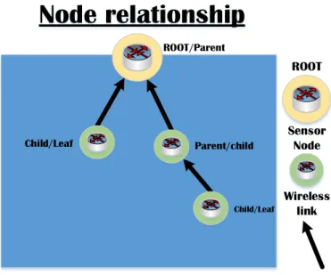
The Routing Protocol for Low-Power and Lossy Networks [21] (RPL) uses the rules of a DAG to create its routing structure. This structure is often described as a tree, with the DAG root at the top of the tree and DAG nodes making up the rest of the tree. Every node is in a parent/child relationship, where the DAG root is a node with no outgoing lines and the endpoint of the graph, therefor it is always a parent and cannot be a child. Every other node in the graph can either be a parent or a child, nodes can however be in more than one relationship at once. What determines whether a node is a parent, or a child is its rank and relative position to its connected nodes. The nodes with highest rank are called leaf's. A node is considered either a parent, child or leaf depending on the decision process called Objective Function. An example of the RPL parent/child relationship can be seen in Figure 5.

(13)

Node relationship

ROOT/Parent Parent/child Child/Leaf Child/Leaf ROOT Sensor Node Wireless link

Figure 5 - Diagram depicting the parent and child relationship in RPL

2.11.1. Objective Function

The rank of a node is determined by the Objective Function [21, p. 11], this is an algorithm that decides what rank a node will get in the routing structure and what type of node it will be. Nodes with a lower rank is topologically closer to the DAG root, it is worth mentioning that physical location of a node can impact its rank, but it is not necessarily important. For example, if the Objective Function heavily depends on latency or signal strength actual distance of the nodes will be of great importance. Figure 6 shows how a physical topology and the RPL tree structure can differ. For each level of parent/child relationship the rank increases. It is up to the developer to construct the Objective Function so that the RPL network acts as intended, to achieve its goal, there is however default values that will construct a tree topology if nothing specific is implemented.

RPL STRUCTURE

ROOT Rank 1 Rank 2

PHYSICAL TOPOLOGY

ROOT Rank 1 Rank 2 Rank 2 Rank 1 Rank 2 ROOT Sensor Node Wireless link

(14)

2.11.2. DODAG Goal

The DODAG Goal is application-specific for every RPL network. A DODAG Goal can for example be to have an overall local network latency below a certain threshold, to minimize the overall energy consumption or to always have the lowest possible amount of different ranks in the tree. The Objective Function should be designed in a way, that the nodes behave accordingly to achieve said goal. The DODAG can be in two different states, and the RPL root advertises which is the case. If the DODAG has achieved its goal it will be in a grounded state, if the network does not have the necessary properties to accomplish the goal it will be set to a floating state, the DODAG can however still provide connectivity to other nodes within the DODAG [21, p. 18].

2.11.3. Use case for RPL

RPL was developed to achieve routing for resource-constraint devices within a network with high packet loss and low data rate, also called Low-power and Lossy Networks, this can for example be a wireless sensor network. For a Wireless Sensor Network, conventional routing protocols such as OSPF or BGP do not work, this is because they are too resource demanding. A Low-powerd and Lossy Network can contain thousands of nodes and the traffic sent can be point-to-point, point-to-multipoint or multipoint-to-point [21, p. 19].

2.12. IEEE 802.15.4 - Low-Rate Wireless Personal Area Networks

IEEE 802.15.4 is a network standard developed by the IEEE Working Group for Wireless Specialty network and is part of the 802.15 class. The protocol is developed for Low-Rate Wireless Personal Area Networks (LR-WPAN) and is designed to be used with low-power consuming wireless devices with extremely low data rates. Wireless sensor nodes and IoT devices often has these limitations, LR-WPAN is therefor suitable to be used with these kinds of devices. The protocol is separated into two different layers, MAC and physical.

The MAC sublayer manages transmission of frames between the physical and upper layers. This is handled through several different functions within the MAC layer. It uses Carrier-Sense Multiple Access with collision avoidance (CSMA/CA) and Time Synchronized Channel Hopping (TSCH) to avoid and reduce different kinds of interference, TSCH also provide low-power properties [22].

The physical layer handles transmission and reception of data on a hardware level, it also detects the link quality and decides which channel frequency to use [23, p. 381]. Clear Channel Assessment uses Carrier Sense and Energy Detection to determine if it is possible to access the medium. Carrier Sense works by listening to wireless signals with a specific modulation and frequency to determine if someone else is transmitting data on a given channel. If a sufficiently strong and valid signal is detected the medium will be reported as busy, otherwise it will be marked as idle and able to start transmitting data. Energy Detection is used to determine if there are any interfering sources in the nearby area. Any form of background noise which exceeds the maximum power level threshold, will mark the medium as busy. This is a mechanism that determines if it is worth, or even possible to transmit data at that moment [23, p. 402].

Radio duty cycle is the amount of time the radio is active before going to sleep. By reducing the duty cycle energy consumption will be reduced, this is managed by activating and

(15)

deactivating the radio transceivers, thus minimizing the battery usage of a device [24, p. 12]. Contiki-OS uses several protocols to manage the radio duty cycle; the ContikiMAC protocol, Contiki X-MAC and Contiki LPP, these have different properties to help lower the energy consumption [25].

Link quality Indicator calculates an approximated link quality for every received transmission by determining the strength of the received signal, either by using Energy detection or with a signal-to-noise ratio [23, p. 402]. Signal-to-noise ratio is the difference between the strength of a received, valid signal and the ambient background noise floor. A greater difference in signal-to-noise ratio results in a stronger signal [26].

The 802.15.4 standard utilize low transfer rates to achieve low power consumption, these transfer rates can be as low as 20 kbit/s up to 250 kbit/s

[27]

. This creates a major problem for IEEE 802.15.4. It is limited to handle big data packets since its standard Maximum Transmission Unit (MTU) size is 127 bytes, with the header accounted for, this leave 44 bytes to the payload. Wireless Sensor Networks typically use IPv6 to address devices [28] and the default IPv6 MTU size is 1280 bytes this creates problems when sending data over 802.15.4. There is a solution to this problem which is IPv6 over Low-Power Wireless Personal Area Networks (6LoWPAN).

2.13. 6LoWPAN

6LoWPAN was developed as an adaptation layer between 802.15.4 and IPv6 to solve problems of MTU size, the use of compression, fragmentation and reassembly of packets solves the problem with the different packet sizes. The header compression is done by compressing common values in the ipv6 header field. IPv6 header fields are compressed by assuming usage of common values. To meet the requirements of the MTU size of IPv6, the frames are fragmented in to several frames to manage the transition and when the frames come from 802.15.4, they reassemble to be sent as IPv6 packages. By implementing 6LoWPAN issues were solved and made it easier to connect IoT devices to the Internet using the established IP architecture [24, pp. 4-5].

(16)

3. Problem Formulation

This Thesis work aims at solving potential problems regarding future development of Industrial Internet of Things devices with regard to Future Factories in the Cloud. The main goal of this work is to evaluate the performance of an industrial IoT network within the scope of Fog computing with mobile IoT devices. The performance evaluations will consider network reliability in terms of packet delivery ratio, and timeliness in terms of packet delay. We envision a system where a Fog-server provides responsive feedback to connected IIoT devices by acting as a mobility controller for the closed-loop control system. In such a system, the Fog-server acts as a local processing unit, where it collects information from the network, and then provides new rules based on network/application requirements. The feedback command updates rules in the network. In this Thesis, we assume that the Fog-server runs a collision avoidance algorithm, where it avoids mobile nodes’ collision in real-time by sending packets to sensor nodes to either stop moving, change speed or direction. We want to show how a Fog-server can function as an extension to a Cloud service and work with wireless sensor networks. We believe that Fog-servers are a natural development for managing and processing time critical data from devices, and therefore decided to:

• Develop and implement a collision avoidance algorithm for a mobility controller in a closed-loop control system between IoT devices and a Fog-server.

• Evaluate network performance in various situations in terms of accuracy and timeliness when dealing with the existence of a Fog-server within a wireless sensor network.

(17)

4. Method

Different methods were used to answer the individual problem formulations of this thesis work. Firstly, a literature study was conducted to review different technologies with the intention of getting an understanding of cloud computing, Fog computing, IIoT, closed-loop control systems, Contiki-OS and the necessary components of Cooja. This was required since a lot of these technologies are used together in different ways. In parallel with the literature study, the process of setting up a lab environment to conduct experiments and gather quantitative data was also initiated. We worked in Cooja, which is a Linux based emulation tool used to debug microcontrollers such as TmoteSky in a wireless sensor network. Here it was possible to create emulated motes that could communicate over RPL. The experiments resulted in a vast amount of data, which was compiled by calculating the minimum, maximum and averages of delay and packet delivery ratio for the individual motes.

(18)

5. Cooja implementation

Cooja was used to create a simulated environment in order to evaluate the performance of our closed-loop control system with regard to network reliability in terms of packet delivery and delay between a Fog-server and a wireless sensor network. The simulations employed a fixed number of RPL nodes depending on the scenario with a single RPL root to act as a Fog-server for all of them. All nodes were of the type TmoteSky. RPL was used as the underlying routing protocol for the simulations with a single RPL root for simplicity. The only purpose for RPL in our case was to enable routing between the Fog-server and client nodes therefore we let the DODAG stay in a floating state since we did not need to configure a specific goal. 6LoWPAN was used to fragment eventual packets that exceeds the maximum MTU size supported by the IEEE 802.15.4 radio link.

5.1. Simulation scrip editor

The simulation script editor is a way to access the Java interface within Cooja, which is done by writing Java code that runs alongside the simulation. This makes it possible to perform GUI actions, either on set timers or based on logical if statements. It also enables interaction with motes via the serial line interface. The simulation scrip editor is a capable tool and can be used to run simulations directly from the terminal window without any graphics, which saves a lot of system resources for large implementations. This can all be automated to run several iterations of an implementation and saving the output to files for later examination or debugging. We used the simulation script editor for two different GUI functions, (i) to get the nodes current position and (ii) to set a new position based on the decision made by the Fog-server. The simulation script was written to look at the terminal output and check for certain strings, getPosition or setPosition. If getPosition was printed to the terminal by an RPL node, the script would answer with the current position. If the string setPosition was printed, the script would format the string and split on a white space, the split string contained two values, x and y cooridinates, which were used to update the position of the node. All communication between the RPL nodes and simulation script went through the serial line interface. A flow chart of the simulation script is descripbed in Figure 7.

Wait of input YIELD Start SetPosistion() If setPosistion If getPosistion GetPosistion() Yes Yes No No

(19)

5.2. RPL node

The RPL nodes emulate physical TmoteSky devices by running C code in Cooja. They can communicate wirelessly with one another and the Fog-server by using RPL and are also able to communicate with Cooja over the serial line interface. This is used to get the current position of a node and move it to a new location based on the decition of the Fog-server. The purpose of the RPL nodes was to collect and transmit its position to the Fog-server and wait for instructions on how to move. It does this by contacting the Cooja interface once every specified time interval depending on the scenario. The time interval, or sampling rate is set by the etimer [29], a clock function counting in milliseconds (ms) which when expired would trigger a getPosition request. At the samt time it would also contact the Fog-server with the new position and wait for a response. When the RPL node detected a response from the Fog-server, a tcpip event would trigger, which is a process in Cooja that handles incoming data streams. Depending on the Fog-servers decision, a new position would be set with setPosition. A flow chart of the RPL node logic is descripbed in figure 8.

Start

getPosistion() Etimer? TCPIP event? setPosistion() Yes Yes No No update Posistion No

Figure 8 - RPL node flow chart

5.3. RPL root

The RPL root, which is also the Fog-server, acts as the mobility controller for the closed-loop control system and is an emulation of a physical TmoteSky running in Cooja just as the RPL nodes. It is designed to monitor the connected RPL node and determine how they should move. It does this by creating a database containing the last known position, and the pre-determined destination of all connected nodes. When a node informs the Fog-server of its new position a tcpip event is triggered, this initiates the movement algorithm and a decition of how the node should move is sent as a reply. The Fog-server also checks for collisions between nodes, we use this data for one part of the performance evaluation. A flow chart of the RPL root logic is descripbed in figure 9.

(20)

RPL-Node

Start

Movement

algorithm

TCPIP

event

Update position

Figure 9 - RPL root flow chart

5.4. Application example

The structure of our closed-loop control system could be applied to work in an industrial environment with automated guided vehicles (AGVs). Here the RPL nodes would be placed on the AGVs with one or more RPL root in the vicinity, they would however most likely not act as a Fog-server. Instead they would simply enable the RPL nodes to reach a remote Fog or cloud server, extending the industry to the Fog. This server would make the decision of how and when any given AGV could and would move based on an improved version of our movement algorithm.

5.5. Simulation scenarios

Data was collected from a total of 80 simulations of different configurations all running for five minutes. The simulations were conducted in a confined space of 10 x 10 m. The reason for this was to determine if, and how, node density affects communication with respect to packet delivery ratio and delay. Packet delivery ratio is the calculated delta between the number of transmitted and received packets from RPL node to RPL root and RPL root to RPL node. Delay is the time between a packet being transmitted until being received by the endpoint, RPL node to RPL root and RPL root to RPL node. The payload size was altered between simulations to see how that would affect performance.

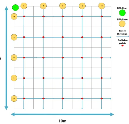
The RPL nodes were positioned on the edges of the grid with a starting distance of two meter apart from one another. Even numbered nodes were placed on the x-axis and odd numbered nodes on the y-axis, in conjunction with the pre-defined destination set by the Fog-server, a known movement pattern for each node could then be calculated. Figure 10 displays an example of how the nodes were positioned. By doing this, we could anticipate where collision would occur and create an estimate of how many collisions statistically would occur within the given simulation time. The result of this is a collision avoidance closed-loop control system between the Fog-server and individual RPL nodes.

(21)

10m 10m

Figure 10 - Diagram of the positioning from scenario five

The amount of collision points is the square of the number of RPL nodes in the simulation divided by two, see Equation 1.

𝑐 = (𝑛𝑢𝑚𝑏𝑒𝑟 𝑜𝑓 𝑛𝑜𝑑𝑒𝑠

2 )

2

(1) Equation 1 – Number of collision points

The nodes were able to move one or two meters at a time per movement, dependant of what the Fog-server calculated. The nodes movement speed can thereby be calculated to be the average movement of 1.5 meter divided by a high estimated delay from the Fog-server of 500ms plus the sampling rate for the current simulation in meter/s, see Equation 2.

𝑠 = 1.5𝑚

500𝑚𝑠 𝑑𝑒𝑙𝑎𝑦 + 𝑠𝑎𝑚𝑝𝑙𝑖𝑛𝑔 𝑟𝑎𝑡𝑒 (2) Equation 2 – Estimated node movement speed

The effective movement speed was however slightly different between nodes due to their sampling rates being 1-10ms out of phase to minimize congestion, this is a miniscule difference and was not considered when compiling the data. With an estimated movement speed and known simulation run time an approximation of the nodes travel distance could be calculated as movement speed multiplied by simulation run time, see Equation 3.

𝑑 = 𝑠 × 𝑠𝑖𝑚𝑢𝑙𝑎𝑡𝑖𝑜𝑛 𝑡𝑖𝑚𝑒 𝑖𝑛 𝑠𝑒𝑐𝑜𝑛𝑑𝑠 (3) Equation 3 – Estimated travel distance

(22)

The average distance nodes need to move before reaching a collision point is half the length in whichever direction they are moving. A rough estimate of the theoretical number of collisions per simulation was calculated based on the above asumptions. Possible travel distance divided by the length of the x or y-axis depending on the nodes travel direction divided by two multiplied by the number of collision points, see Equation 4.

𝑁_𝑐 = 𝑑 (𝑎𝑥𝑖𝑥 𝑙𝑒𝑛𝑔𝑡ℎ₂ )

× 𝑐 (4) Equation 4 – Estimated number of collision

The number of RPL nodes separates the scenarios, scenario one consists of two RPL nodes and one RPL root, scenario two increases the number of RPL nodes to four and so on up to scenario five with ten RPL nodes. Each scenario runs four simulations with alternating sampling rates between 100 – 1000ms aswell as an alternating payload sizes between 8 – 44 byte, this totals 16 different simulations per scenario as seen in Table 2 and 80 simulations overall.

Scenarios Scenario 1 Scenario 2 Scenario 3 Scenario 4 Scenario 5

Number of nodes 2 4 6 8 10

Sampling rate (ms) 100 - 1000 100 - 1000 100 - 1000 100 - 1000 100 - 1000

Payload Size (byte)

8 8 8 8 8

20 20 20 20 20

30 30 30 30 30

44 44 44 44 44

Table 2 - Scenario parameters

Based on the above assumptions we have constructed the following hypotheses; (i) more

nodes will lead to more collisions (ii) more nodes will lead to higher delay (iii) larger payload size will lead to higher delay (iv) higher sampling rate will lead to higher packet loss.

(23)

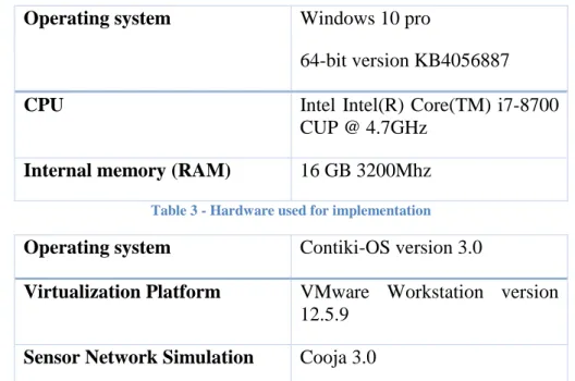
5.6. Hardware and software used in Cooja implementation

The host hardware and software used during implementation and evaluation can be seen in Table 3 and 4.

Operating system Windows 10 pro

64-bit version KB4056887

CPU Intel Intel(R) Core(TM) i7-8700 CUP @ 4.7GHz

Internal memory (RAM) 16 GB 3200Mhz

Table 3 - Hardware used for implementation

Operating system Contiki-OS version 3.0

Virtualization Platform VMware Workstation version

12.5.9

Sensor Network Simulation Cooja 3.0

(24)

6. Result

The results of the data obtained using the tests are presented in graphs with a brief explanation of what the graph means and a shorter analysis of these. A brief summary of all results will be specified at the end of this section.

6.1. Scenario 1

Figure 11 shows how delay is affected by different payload sizes. The results reveal that there is no noticeable impact on the end-to-end delay when the packet size went from 8 bytes to 44 bytes.

Figure 11 - Delay with respect to payload size for two RPL nodes

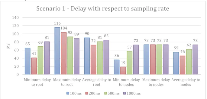
Figure 12 show how delay is affected by different sampling rates, there is a noticeable difference between simulations with two RPL nodes, a sampling rate of 200ms leads the lowest delay.

Figure 12 - Delay with respect to sampling rate for two RPL nodes

64 99 82 46 74 60 64 102 83 45 74 59 64 101 83 46 74 60 64 99 81 46 73 60 0 20 40 60 80 100 120 Minimum delay

to root Maximum delayto root Average delay toroot Minimum delayto nodes Maximum delayto nodes Average delay tonodes

MS

Scenario 1 - Delay with respect to payload size

8(byte) 20(byte) 30(byte) 44(byte)

65 116 90 36 73 55 41 104 72 19 73 46 69 93 81 57 73 62 81 89 85 73 73 73 0 20 40 60 80 100 120 140 Minimum delay

MS

Scenario 1 - Delay with respect to sampling rate

(25)

Figure 13 show how packet loss is affected by different payload sizes, there is no noticeable difference between simulations with two RPL nodes.

Figure 13 - Packet loss with respect to payload size for two RPL nodes

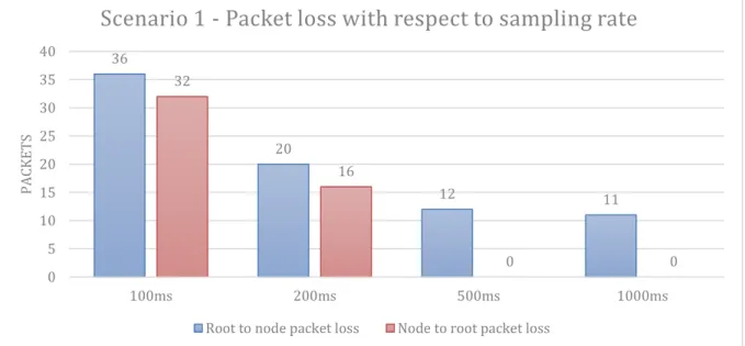
Figure 14 show how packet loss is affected by different sampling rates, there is a considerable difference between simulations with two RPL nodes, where a sampling rate of 100ms has the most packet loss.

Figure 14 - Packet loss with respect to sampling size for two RPL nodes

20 20 20 ₁₉ 11 11 11 12 0 5 10 15 20 25

8byte 20byte 30byte 44byte

PA

CKE

T

S

Scenario 1 - Packet loss with respect to payload size

Root to node packet loss Node to root packet loss

36 20 12 ₁₁ 32 16 0 0 0 5 10 15 20 25 30 35 40 100ms 200ms 500ms 1000ms PA CKE T S

Scenario 1 - Packet loss with respect to sampling rate

(26)

Figure 15 show how packet delivery is affected by different payload sizes, there is no noticeable difference between simulations with two RPL nodes.

Figure 15 - Packet delivery with respect to payload size for two RPL nodes

Figure 16 show how packet delivery is affected by different sampling rates, there is no noticeable difference between simulations with two RPL nodes.

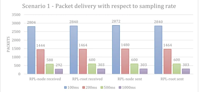
Figure 16 - Packet delivery with respect to sampling rate for two RPL nodes

1282 1302 1313 1302 1282 1302 1313 1302 1282 1302 1313 1302 1282 1301 1313 1301 1265 1270 1275 1280 1285 1290 1295 1300 1305 1310 1315 1320

RPL-node received RPL-root received RPL-node sent RPL-root sent

PA

CKE

T

S

Scenario 1 - Packet delivery with respect to payload size

2804 2840 2872 2840 1444 1464 1480 1464 588 600 600 600 292 303 303 303 0 500 1000 1500 2000 2500 3000 3500

PA

CKE

T

S

Scenario 1 - Packet delivery with respect to sampling rate

(27)

Figure 17 show how the packet delivery ratio is affected by different payload sizes, there is no noticeable difference between simulations with two RPL nodes.

Figure 17 - Packet delivery ratio with respect to payload size for two RPL nodes

Figure 18 show how the packet delivery ratio is affected by different payload sizes, there is no noticeable difference between simulations with two RPL nodes.

Figure 18 - Packet delivery ratio with respect to sampling rate for two RPL nodes

98% 98% 98% 99%

99% 99% 99%

99%

R

A

T

IO

Scenario 1 - Packet delivery ratio with respect to payload

size

Root to node ratio Node to root ratio

99% _99% 98% 96% 99% 99% 100% 100% 100ms 200ms 500ms 1000ms R A T IO

Scenario 1 - Packet delivery ratio with respect to

sampling rate

(28)

6.2. Scenario 2

Figure 19 show how delay is affected by different payload sizes, there is no noticeable difference between simulations with four RPL nodes.

Figure 19 - Delay with respect to payload size for four RPL nodes

Figure 20 show how delay is affected by different sampling rates, there is a noticeable difference between simulations with four RPL nodes for the minimum and maximum delay.

Figure 20 - Delay with respect to sampling rate for four RPL nodes

34 81 58 15 60 62 35 76 56 16 58 37 34 74 54 17 58 37 34 91 63 13 62 38 0 10 20 30 40 50 60 70 80 90 100 Minimum delay

MS

Scenario 2 - Delay with respect to payload size

27 89 58 6 75 58 25 78 52 12 54 33 42 88 65 19 48 34 45 67 56 19 46 33 0 10 20 30 40 50 60 70 80 90 100 Minimum delay

MS

Scenario 2 - Delay with respect to sampling rate

(29)

Figure 21 show how packet loss is affected by different payload sizes, there is a considerable difference between simulations with four RPL nodes with a payload size of 30 bytes.

Figure 21 - Packet loss with respect to payload size for four RPL nodes

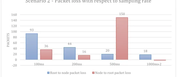
Figure 22 show how packet loss is affected by different sampling rates, there is a considerable difference between simulations with four RPL nodes for 100 and 500ms.

Figure 22 - Packet loss with respect to sampling rate for four RPL nodes

44 45 ₄₂ 44 12 12 88 13 0 10 20 30 40 50 60 70 80 90 100

PA

CKE

T

S

Scenario 2 - Packet loss with respect to payload size

93 44 20 18 36 16 150 -2 -20 0 20 40 60 80 100 120 140 160 100ms 200ms 500ms 1000ms PA CKE T S

Scenario 2 - Packet loss with respect to sampling rate

(30)

Figure 23 show how packet delivery is affected by different payload sizes, there is a noticeable difference between simulations with four RPL nodes with a payload size of 30byte.

Figure 23 - Packet delivery with respect to payload size for four RPL nodes

Figure 24 show how packet delivery is affected by different sampling rates, there is no noticeable difference between simulations with four RPL nodes.

Figure 24 - Packet delivery with respect to sampling rate for four RPL nodes

2587 2631 2643 2631 2587 2632 2644 2632 2589 2631 2719 2631 2586 2630 2643 2630 2500 2550 2600 2650 2700 2750

PA

CKT

ES

Scenario 2 - Packet delivery with respect to payload size

5669 5762 5798 5762 2912 2956 2972 2956 1184 1204 1354 1204 584 602 600 602 0 1000 2000 3000 4000 5000 6000 7000

PA

CKE

T

S

Scenario 2 - Packet delivery with respect to sampling rate

(31)

Figure 25 show how the packet delivery ratio is affected by different payload sizes, there is no noticeable difference between simulations with four RPL nodes.

Figure 25 - Packet delivery Ratio with respect to payload size for four RPL nodes

Figure 26 show how the packet delivery ratio is affected by different sampling rates, there is a noticeable difference between simulations with four RPL nodes with a sampling rate of 500ms.

Figure 26 - Packet delivery Ratio with respect to sampling rate for four RPL nodes

98% 98% 98% 98%

100% 100%

97%

100%

R

A

T

IO

Scenario 2 - Packet delivery Ratio with respect to payload

size

98% 99% 99% 99% 98% _97% 89% 100% 100ms 200ms 500ms 1000ms R A T IO

Scenario 2 - Packet delivery Ratio with respect to

sampling rate

(32)

6.3. Scenario 3

Figure 27 show how delay is affected by different payload sizes, there is a noticeable difference between simulations with four RPL nodes with payload sizes of 8 and 30 byte.

Figure 27 - Delay with respect to payload size for six RPL nodes

Figure 28 show how delay is affected by different sampling rates, there is a significant difference in maximum delay between simulations with four RPL nodes with a sampling rate of 100ms

Figure 28 - Delay with respect to sampling rate for six RPL nodes

18 99 58 14 105 59 14 85 50 17 133 75 15 57 36 19 125 72 15 63 39 17 140 79 0 20 40 60 80 100 120 140 160 Minimum delay

MS

Scenario 3 - Delay with respect to payload size

10 90 50 9 284 146 10 61 36 19 97 58 18 76 47 21 91 56 18 38 28 20 50 35 0 50 100 150 200 250 300 Minimum delay

MS

Scenario 3 - Delay with respect to sampling rate

(33)

Figure 29 show how packet loss is affected by different payload sizes, there is a significant difference between simulations with four RPL nodes with a payload size of 30 and 44 byte.

Figure 29 - Packet loss with respect to payload size for six RPL nodes

Figure 30 show how packet loss is affected by different sampling rates, there is an enormous difference between simulations of four RPL nodes with a sampling rate of 500ms.

Figure 30 - Packet loss with respect to sampling rate for six RPL nodes

222 221 241 257 31 30 1 326 0 50 100 150 200 250 300 350

PA

CKE

T

S

Scenario 3 - Packet loss with respect to payload size

806 76 2648 889 86 ₄₀ 2616 60 0 500 1000 1500 2000 2500 3000 100ms 200ms 500ms 1000ms PA CKE T S

Scenario 3 - Packet loss with respect to sampling rate

(34)

Figure 31 show how packet delivery is affected by different payload sizes, there is a considerable difference between simulations with four RPL nodes and a payload size of 44 byte for packets received by the RPL root.

Figure 31 - Packet delivery with respect to payload size for six RPL nodes

Figure 32 show how packet delivery is affected by different sampling rates, there is no noticeable difference between simulations with four RPL nodes.

Figure 32 - Packet delivery with respect to sampling rate for six RPL nodes

3720 3942 3973 3942 3723 3944 3974 3944 3703 3943 3944 3944 3683 3647 3973 3940 3400 3500 3600 3700 3800 3900 4000

PA

CKE

T

S

Scenario 3 - Packet delivery with respect to payload size

7830 8636 8722 8636 4348 4424 4464 4424 1776 1808 4424 4424 875 840 900 1764 0 1000 2000 3000 4000 5000 6000 7000 8000 9000 10000

PA

CKE

T

S

Scenario 3 - Packet delivery with respect to sampling rate

(35)

Figure 33 show how the packet delivery ratio is affected by different payload sizes, there is a noticeable difference between simulations with four RPL nodes and a payload size of 44 byte from RPL node to RPL root.

Figure 33 - Packet delivery ratio with respect to payload size for six RPL nodes

Figure 34 show how the packet delivery ratio is affected by different sampling sizes, there is a significant difference between simulations with four RP-nodes and a sampling rate of 500ms.

Figure 34 - Packet delivery Ratio with respect to sampling rate for six RPL nodes

94% 94% _94%

93%

99% 99% 100%

92%

R

A

T

IO

Scenario 3 - Packet delivery ratio with respect to payload

size

91% 98% 40% 50% 99% 99% 41% 93% 100ms 200ms 500ms 1000ms R A T IO

Scenario 3 - Packet delivery Ratio with respect to

sampling rate

(36)

6.4. Scenario 4

Figure 35 show how delay is affected by different payload sizes, there is no noticeable difference between simulations with six RPL nodes.

Figure 35 - Delay with respect to payload size for eight RPL nodes

Figure 36 show how delay is affected by different sampling rates, there is a significant difference between simulations with six RPL nodes and a sampling rate of 100ms.

Figure 36 - Delay with respect to sampling rate for eight RPL nodes

39 103 71 6 145 76 38 106 72 6 137 72 38 111 75 7 128 67 39 118 79 6 144 75 0 20 40 60 80 100 120 140 160 Minimum delay

MS

Scenario 4 - Delay with respect to payload size

32 173 102 4 327 165 37 103 70 5 105 55 41 80 61 8 64 36 45 82 64 9 58 33 0 50 100 150 200 250 300 350 Minimum delay

MS

Scenario 4 - Delay with respect to sampling rate

(37)

Figure 37 show how packet loss is affected by different payload sizes, there is no noticeable difference between simulations with six RPL nodes.

Figure 37 - Packet loss with respect to payload size for eight RPL nodes

Figure 38 show how packet loss is affected by different sampling rates, there is a significant difference between simulations with six RPL nodes over all except for a sampling rate of 500ms.

Figure 38 - Packet loss with respect to sampling rate for eight RPL nodes

924 928 1036 ₁₀₀₅ 22 25 24 26 0 200 400 600 800 1000 1200

PA

CKE

T

S

Scenario 4 - Packet loss with respect to payload size

3605 163 2113 1219 71 29 2064 1 0 500 1000 1500 2000 2500 3000 3500 4000 100ms 200ms 500ms 1000ms PA CKE T S

Scenario 4 - Packet loss with respect to sampling rate

(38)

Figure 39 show how packet delivery is affected by different payload sizes, there is no noticeable difference between simulations with six RPL nodes.

Figure 39 - Packet delivery with respect to payload size for eight RPL nodes

Figure 40 show how packet delivery is affected by different sampling rates, there is no noticeable difference between simulations with six RPL nodes.

Figure 40 - Packet delivery with respect to sampling rate for eight RPL nodes

4343 5267 5289 5267 4340 5268 5293 5268 4257 5269 5293 5293 4260 5265 5291 5265 0 1000 2000 3000 4000 5000 6000

PA

CKE

T

S

Scenario 4 - Packet delivery with respect to payload size

7931 11536 11607 11536 5757 5920 5949 5920 2359 2408 4472 4472 1153 1205 1204 2372 0 2000 4000 6000 8000 10000 12000 14000

PA

CKE

T

S

Scenario 4 - Packet delivery with respect to sampling rate

(39)

Figure 41 show how the packet delivery ratio is affected by different payload sizes, there is no noticeable difference between simulations with six RPL nodes.

Figure 41 - Packet delivery Ratio with respect to payload size for eight RPL nodes

Figure 42 show how the packet delivery ratio is affected by different sampling rates, there is a considerable difference between simulations with six RPL nodes and a sampling rate of 500ms.

Figure 42 - Packet delivery ratio with respect to sampling rate for eight RPL nodes

82% 82% _80% 81%

100% 100% 100% 100%

R

A

T

IO

Scenario 4 - Packet delivery Ratio with respect to payload

size

69% 97% 53% _49% 99% 100% 54% 100% 100ms 200ms 500ms 1000ms R A T IO

Scenartio 4 - Packet delivery ratio with respect to

sampling rate

(40)

6.5. Scenario 5

Figure 43 show how delay is affected by different payload sizes, there is no noticeable difference between simulations with ten RPL nodes.

Figure 43 - Delay with respect to payload size for ten RPL nodes

Figure 44 show how delay is affected by different sampling rates, there is a considerable difference between the maximum delay to nodes is simulations with ten RPL nodes and a sampling rate of 100 ms.

Figure 44 - Delay with respect to sampling rate for ten RPL nodes

9 73 41 ₃₅ 216 126 8 73 40 ₃₃ 231 132 8 74 41 ₃₃ 209 121 6 72 39 ₃₄ 220 127 0 50 100 150 200 250 Minimum delay

MS

Scenario 5 - Delay with respect to payload size

2 128 65 22 398 210 4 66 35 36 209 123 11 48 30 38 144 91 13 51 32 38 126 82 0 50 100 150 200 250 300 350 400 450 Minimum delay

MS

Scenario 5 - Delay with respect to sampling rate

(41)

Figure 45 show how packet loss is affected by different payload sizes, there is no noticeable difference between simulations with ten RPL nodes.

Figure 45 - Packet loss with respect to payload size for ten RPL nodes

Figure 46 show how packet loss is affected by different sampling rates, there is an enormous difference in simulations with ten RPL nodes and a sampling rates of 100ms.

Figure 46 - Packet loss with respect to sampling rate for ten RPL nodes

1815 1832 1928 1989 41 39 37 42 0 500 1000 1500 2000 2500

PA

CKE

T

S

Scenario 5 - Packet loss with respect to payload size

6911 491 83 79 98 61 0 0 0 1000 2000 3000 4000 5000 6000 7000 8000 100ms 200ms 500ms 1000ms PA CKE T S

Scenario 5 - Packet loss with respect to sampling rate

(42)

Figure 47 show how packet delivery is affected by different payload sizes, there is no noticeable difference between simulations with ten RPL nodes.

Figure 47 - Packet delivery with respect to payload size for ten RPL nodes

Figure 48 show how packet delivery is affected by different sampling rates, there is no noticeable difference between simulations with two RPL nodes.

Figure 48 - Packet delivery with respect to Sampling rate for ten RPL nodes

4747 6562 6603 6562 4730 6562 6601 6562 4636 6564 6601 6564 4576 6565 6607 6565 0 1000 2000 3000 4000 5000 6000 7000

PA

CKE

T

S

Scenario 5 - Packet delivery with respect to payload size

7456 14367 14465 14367 6879 7370 7431 7370 2925 3008 3008 3008 1429 1508 1508 1508 0 2000 4000 6000 8000 10000 12000 14000 16000

PA

CKE

T

S

Scenario 5 - Packet delivery with respect to Sampling rate

(43)

Figure 49 show how the packet delivery ratio is affected by different payload sizes, there is no noticeable difference between simulations with ten RPL nodes.

Figure 49 - Packet delivery ratio with respect to payload size for ten RPL nodes

Figure 50 show how the packet delivery ratio is affected by different sampling rates, there is a significant difference in simulations with ten RPL nodes and a sampling rate of 100ms between RPL node and RPL root.

Figure 50 - Packet delivery ratio with respect to sampling rate for ten RPL nodes

72% 72% 71% 70%

99% 99% 99% 99%

R

A

T

IO

Scenario 5 - Packet delivery ratio with respect to payload

size

52% 93% 97% 95% 99% 99% 100% 100% 100ms 200ms 500ms 1000ms R A T IO

Scenario 5 - Packet delivery ratio with respect to

sampling rate

(44)

6.6. Collisions

Figure 51 show the theoretical number of expected collisions based on the calculations made in chapter 5.5 on Simulation scenarios.

Figur 51 - Theoretical number of collisions for all scenarios

Figure 52 show the number of collisions that occurred for each simulated scenario. There is a noticeable trend and linear growth with an increasing number of nodes per simulation. The practical simulations show much fewer collisions compared to the theoretical estimate, with peek performance of 91% reduced number of collision for scenario 1 with the collision avoidance algorithm running.

Figure 52 – Practical number of collisions for all scenarios

429 1714 4204 7474 10714 60 240 540 960 1500 150 600 1350 2400 3750 86 343 841 1495 2143 0 2000 4000 6000 8000 10000 12000

Scenario 1 Scenario 2 Scenario 3 Scenario 4 Scenario 5

COL

LI

SI

ONS

All scenarios - Theoretical number of collisions

Total number of collisions Minimum number of collisions Maximum number of collisions Average number of collisions

38 186 569 705 1250 0 8 1 48 7 82 0 121 10 197 2 12 36 44 78 0 200 400 600 800 1000 1200 1400

Scenario 1 Scenario 2 Scenario 3 Scenario 4 Scenario 5

COL

LI

SI

ONS

All scenarios - Practical number of collisions

Total number of collision Minimum number of collision Maximum number of collision Average number of collision

Evaluating the functionality of an Industrial Internet of Things system in the Fog

V

,

S

T

D

B

S

E

–

C

N

E

15.0

C

E

VALUATING THE FUNCTIONALITY OF AN

I

NDUSTRIAL

I

NTERNET OF

T

HINGS SYSTEM

IN THE

F

OG

mgd15001@student.mdh.se

che15001@student.mdh.se

Examiner:

Moris Behnam

Supervisor: Hossein Fotouhi

Abstract

Table of Contents

1. Introduction

2. Background

Node relationship

RPL STRUCTURE

PHYSICAL TOPOLOGY

[27]

3. Problem Formulation

4. Method

5. Cooja implementation

Start

RPL-Node

Start

Movement

algorithm

TCPIP

event

Update position

6. Result

Scenario 1 - Delay with respect to payload size

Scenario 1 - Delay with respect to sampling rate

Scenario 1 - Packet loss with respect to payload size

Scenario 1 - Packet loss with respect to sampling rate

Scenario 1 - Packet delivery with respect to payload size

Scenario 1 - Packet delivery with respect to sampling rate

Scenario 1 - Packet delivery ratio with respect to payload

size

Scenario 1 - Packet delivery ratio with respect to

sampling rate

Scenario 2 - Delay with respect to payload size

Scenario 2 - Delay with respect to sampling rate

Scenario 2 - Packet loss with respect to payload size

Scenario 2 - Packet loss with respect to sampling rate

Scenario 2 - Packet delivery with respect to payload size

Scenario 2 - Packet delivery with respect to sampling rate

Scenario 2 - Packet delivery Ratio with respect to payload

size

Scenario 2 - Packet delivery Ratio with respect to

sampling rate

Scenario 3 - Delay with respect to payload size

Scenario 3 - Delay with respect to sampling rate

Scenario 3 - Packet loss with respect to payload size

Scenario 3 - Packet loss with respect to sampling rate

Scenario 3 - Packet delivery with respect to payload size

Scenario 3 - Packet delivery with respect to sampling rate

Scenario 3 - Packet delivery ratio with respect to payload

size

Scenario 3 - Packet delivery Ratio with respect to