Electronic Research Archive of Blekinge Institute of Technology
http://www.bth.se/fou/
This is an author produced version of a journal paper. The paper has been peer-reviewed but
may not include the final publisher proof-corrections or journal pagination.
Citation for the published Journal paper:
Title:
Author:
Journal:
Year:
Vol.
Issue:
Pagination:
URL/DOI to the paper:
Access to the published version may require subscription.
Published with permission from:
Prediction of faults-slip-through in large software projects: an empirical evaluation
Wasif Afzal, Richard Torkar, Robert Feldt, Tony Gorschek
Software Quality Journal
51-86
1
22
2014
10.1007/s11219-013-9205-3
Springer
(will be inserted by the editor)
Prediction of faults-slip-through in large software
projects: An empirical evaluation
Wasif Afzal · Richard Torkar · Robert Feldt · Tony Gorschek
Received: date / Accepted: date
Abstract BACKGROUND – A large percentage of the cost of rework can be avoided by finding more faults earlier in a software test process. There-fore, determination of which software test phases to focus improvement work on, has considerable industrial interest. OBJECTIVE AND METHOD – We evaluate a number of prediction techniques for predicting the number of faults slipping through to unit, function, integration and system test phases of a large industrial project. The objective is to quantify improvement potential in different test phases by striving towards finding the faults in the right phase. RESULTS – The results show that a range of techniques are found to be useful in predicting the number of faults slipping through to the four test phases, however, the group of search-based techniques (genetic programming Wasif Afzal
Department of Computer Sciences Bahria University
Shangrilla Road, Sector E-8, 44000, Islamabad, Pakistan. Tel.: +92-51-9260002 Fax: +92-51-9260885
E-mail: wasif.afzal@gmail.com Richard Torkar and Robert Feldt
Department of Computer Science and Engineering Chalmers University of Technology, 41296, Gothenburg, Sweden.
and
School of Computing
Blekinge Institute of Technology, 37179, Karlskrona, Sweden.
E-mail: richard.torkar—robert.feldt@chalmers.se Tony Gorschek
School of Computing
Blekinge Institute of Technology, 37179, Karlskrona, Sweden.
(GP), gene expression programming (GEP), artificial immune recognition sys-tem (AIRS) and particle swarm optimization based artificial neural network (PSO-ANN)) consistently give better predictions, having a representation at all of the test phases. Human predictions are consistently better at two of the four test phases. CONCLUSIONS – We conclude that the human predictions regarding the number of faults slipping through to various test phases can be well supported by the use of search-based techniques. A combination of human and an automated search mechanism like any of the search-based techniques has the potential to provide improved prediction results.
Keywords Prediction, Empirical, Faults-slip-through, Search-based
1 Introduction and problem statement
Presence of a number of faults1usually indicates an absence of software quality.
Software testing is the major fault-finding activity, therefore much research has focused on making the software test process as efficient and as effective as pos-sible. One way to improve the test process efficiency is to avoid unnecessary re-work by finding more faults earlier. This argument is based on the premise that the faults are cheaper to find and remove earlier in the software development process (Boehm and Basili, 2001). Faults-slip-through (FST) metric (Damm et al, 2006; Damm, 2007) is one way of providing quantified decision support to reduce the effort spent on rework.
Faults-slip-through (FST) metric is used for determining whether a fault slipped through the phase where it should have been found or not (Damm et al, 2006; Damm, 2007). The term phase refers to any phase in a typical software development life cycle (ISO/IEC 12207 (std, 2008) defines the differ-ent software developmdiffer-ent phases). However the most interesting and industry-supported applications of FST measurement are in the test phase of a software development life cycle, because it is typically in this phase where the faults are classified into their actual and expected identification phases.
The time between when a fault was inserted and found is commonly re-ferred to as ‘fault latency’ (Hribar, 2008). Fig. 1 shows the difference between fault latency and FST (Damm et al, 2006; Damm, 2007). As it is clear from this figure, the FST measurement evaluates when it is cost efficient to find a certain fault. To be able to specify this, the organization must first determine what should be tested in which phase (Damm et al, 2006; Damm, 2007).
Studies on multiple projects executed within several different organizations at Ericsson (Damm, 2007) showed that FST measurement has some promising advantages:
1. FST can prioritize which phases and activities to improve.
2. The FST measurement approach can assess to which degree a process achieves early and cost-effective software fault detection (one of the studies
1 According to IEEE Standard Glossary of Software Engineering Terminology (iee, 1990),
Design Coding Unit test Function Test System Test Operation = When fault was inserted
= When fault was found and corrected
= FST fault belonging (when most cost-effective to find)
Fault latency
Fault slippage
Figure 2.1: Example of Fault Latency and FST
found in which phase. To be able to specify this, the organization must first determine what should be tested in which phase. Therefore, this can be seen as test strategy work. Thus, experienced developers, testers and managers should be involved in the creation of the definition. The results of the case study in Section 2.3 further exemplify how to create such a definition. Table 2.1 provides a fictitious example of FST between arbitrarily chosen development phases. The columns represent in which phase the faults were found (phase found) and the rows represent where the faults should have been found (phase belonging). For example, 25 of the faults that were found in function test should have been found during unit test (e.g. through inspections or unit tests). Further, the rightmost column summarizes the amount of faults that belonged to each phase whereas the bottom row summarizes the amount of faults that were found in each phase. For example, 49 faults belonged to the unit test phase whereas most of the faults were found in function test (50).
2.2.2 Average Fault Cost
When having all the faults categorized, the next step is to estimate the cost of finding faults in different phases. Several studies have shown that the cost of finding and fixing faults increases more and more the longer they remain in a product (Boehm
49
Fig. 1 Difference between fault latency and FST.
indicated that it is possible to obtain good indications of the quality of the test process already when 20–30% of the faults have been found).
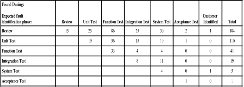
Fig. 2 shows an example snippet of a faults-slip-through matrix showing the faults slipping through to later phases. The columns in Fig. 2 represent the phases in which the faults were found (Found During ) whereas the rows represent the phases where the faults should have been found (Expected fault identification phase). For example, 56 of the faults that were found in the function test should have been found during the unit test.
Report Name: Fault Slip Through Analysis Project: FST M570 Start Date: 2009-06-22 End Date: 2009-12-13 Customer Delivery: 2009-12-22
FST Measurement Tool
FST Matrix Found During:
Expected fault
identification phase: Review Unit Test Function Test Integration Test System Test Acceptance Test
Customer Identified Total Output Slippage% Review 15 25 86 25 30 2 1 184 47 Unit Test 19 56 15 19 1 0 110 25 Function Test 33 4 4 0 0 41 2 Integration Test 8 11 0 0 19 3 System Test 4 0 1 5 0 Acceptence Test 1 0 1 0 Total 15 44 175 52 68 4 2 360 Input Slippage % 0 57 81 85 94 75 100 0
Review Unit Test Function Test Integration Test System Test Acceptance Test Customer
Identified Total Incorrect data 76 1 8 25 1 0 0 0 111 24% Review Unit Test Function Test Integration Test System Test Acceptance Test Customer Identified
System Design Review, Module Design Review, Code Review HW Development, System Simulation, Module Test Function Test, Interoperability development test Integration of modules to functions, Integration Test System Test, IOT, Delivery Test
Type Approval
Customization, Customer Acceptance, Operator Identified, Customer Identified Fig. 2 An example FST matrix.
Apart from the studies done by Damm (Damm et al, 2006; Damm, 2007), there are other studies on successful industrial implementation of FST mea-surements. Two such cases are the FST implementations at Ericsson Nikola
Tesla (Hribar, 2008; ˇZ. Antoli´c, 2007). They started collecting FST
measure-ments in all development projects from the middle of the year 2006. The results were encouraging with a decrease of fault-slippage to customers, improvements of test configurations and improvements of test cases used in the verification phase of the projects.
Considering the initial successful results of implementing FST measure-ment across different organizations within Ericsson, our industrial partner
be-came interested in investigating how to use FST measurement to provide addi-tional decision support for project management. For example, Staron and Med-ing (Staron and MedMed-ing, 2008) highlight that the prediction of the number of faults slipping through can be a refinement to their proposed approach for pre-dicting the number of defects in the defect database. Similarly Damm (Damm, 2007) highlight that FST measurement can potentially be used as a support tool in software fault predictions. This additional decision support is to make the software development more predictable (Rakitin, 2001).
The number of faults found by the test team impacts whether or not a project would be completed on schedule and with a certain quality. The project manager has to balance the resources, not only for fixing the identified faults, but also to implement any new functionality. This balance has to be distributed correctly on a weekly or a monthly basis. Any failure to achieve this balance would mean that either the project team is late with the project delivery or the team resources are kept under-utilized.
In this paper, we focus on predicting the number of faults slipping through to different test phases, multiple weeks in advance (a quantitative modeling
task). We compare a variety of prediction techniques2. Since there is a general
lack of empirical evaluation of expert judgement (Tomaszewski et al, 2007; Catal and Diri, 2009) and due to the fact that predictions regarding software quality are based on expert judgements at our organization, and we would argue in industry in general, we specifically compare human expert predictions with these techniques. Thus the motivation of doing this study is to:
– avoid predictable pitfalls like effort/schedule over-runs, under-utilization of resources and a large percentage of rework.
– provide better decision-support to the project manager so that faults are prevented early in the software development process.
– prioritize which phases and activities to improve.
The quantitative data modeling make use of several independent variables at the project level, i.e., variables depicting work status, testing progress status and fault-inflow. The dependent variables of interest is then the number of faults slipping through to various test phases, predicted multiple weeks in advance.
Hence, we are interested in answering the following research questions: RQ.1 How do different techniques compare in FST prediction performance? RQ.2 Can other techniques better predict the number of faults slipping through
to different test phases than human expert judgement?
2 statistical techniques (multiple regression, pace regression), tree-structured techniques
(M5P, REPTree), nearest neighbor techniques (K-Star, K-nearest neighbor), ensemble tech-niques (bagging and rotation forest), machine-learning techtech-niques (support vector machines and back-propagation artificial neural networks), search-based techniques (genetic program-ming, artificial immune recognition systems, particle-swarm optimization based artificial neural networks and gene-expression programming) and expert judgement
The data used in the quantitative data modeling comes from large and complex software projects from the telecommunications industry, as our ob-jective is to come up with results that are representative of real industrial use. Also large-scale projects offer different kinds of challenges, e.g., the factors affecting the projects are diverse and many, data is distributed across different systems and success is dependent on the effort of many resources. Moreover, a large project constitutes a less predictable environment and there is a lack of research on how to use predictive models in such an environment (Jørgensen et al, 2000).
We also would like to mention that this study is an extended version of the authors’ earlier conference manuscript (Afzal et al, 2010) where only a limited number of techniques were compared with no evaluation of expert judgement. The rest of the paper is organized as follows. Section 2 summarizes the related work. Section 3 describes the study context, variables selection, the test phases under consideration, the performance evaluation measures and the techniques used. Section 4 presents a quantitative evaluation of various techniques for the prediction task. The results from the quantitative evaluation of different models are discussed in Section 5 while the study validity threats are given in Section 6. The paper is concluded in Section 7 while Appendix A outlines the parameter settings for the different techniques.
2 Related work
Due to the definition of software quality in many different ways, previous studies have focused on predicting different but related dependent variables of interest; examples include predicting for defect density (Nagappan and Ball, 2005; Mohagheghi et al, 2004), software defect content estimation (Briand et al, 2000; Weyuker et al, 2010), fault-proneness (Lessmann et al, 2008; Ar-isholm et al, 2010) and software reliability prediction in terms of time-to-failure (Lyu, 1996). In addition, several independent variables have been used to predict the above dependent variables of interest; examples include predic-tion using size and complexity metrics (Gyimothy et al, 2005), testing met-rics (Veevers and Marshall, 1994; Tomaszewski et al, 2007) and organizational metrics (Nagappan et al, 2008). The actual prediction is performed using a variety of approaches, and can broadly be classified into statistical regression techniques, machine learning approaches and mixed algorithms (Challagulla et al, 2005). Increasingly, evolutionary and bio–inspired approaches are being used for software quality classification (Liu et al, 2010; Afzal and Torkar, 2008) while expert judgement is used in very few studies (Tomaszewski et al, 2007; Zhong et al, 2004).
For a more detailed overview of related work on software fault prediction studies, the reader is referred to (Tian, 2004; Fenton and Neil, 1999; Catal and Diri, 2009; Wagner, 2006; Runeson et al, 2006).
This study is different from the above software quality evaluation studies. First, the dependent variable of interest for the quantitative data modeling
is the number of faults slipping through to various test phases, with the aim of taking corrective actions for avoiding unnecessary rework late in software testing. Second, the independent variables of interest for the quantitative data modeling are diverse and at the project level, i.e., variables depicting work sta-tus, testing progress status and fault-inflow (shown later in Table 1). A similar set of variables were used in a study by Staron and Meding (Staron and Med-ing, 2008), but predicted weekly defect inflow and used different techniques. Third, for the sake of comparison, we include a variety of carefully selected techniques, representing both commonly used and newer approaches.
Together this means our study is broader and more industrially relevant than previous studies.
3 Study plan
This section describes the context, independent/dependent variables for the prediction model, the research method, the predictive performance measures and the techniques used for quantitative data modeling.
3.1 Study context
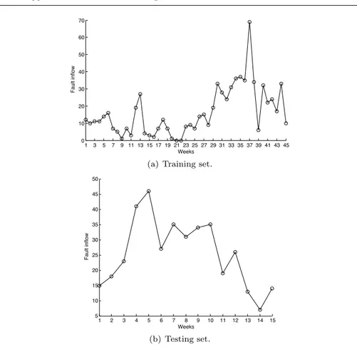
As given in Section 1, our context is large and complex software projects in the telecommunications industry. Our subject company develops mobile platforms and wireless semiconductors. The projects are aimed at developing platforms introducing new radio access technologies written using the C programming language. The average number of persons involved in these projects is approx-imately 250. Since the project are from a similar domain, the data from one of the projects is used as a baseline to train the models while the data from the second project is used to evaluate the models’ results. We have data from 45 weeks of the baseline project to train the models while we evaluate the results on data from 15 weeks of an on-going project. Fig. 3 shows the number of faults occurring per week for the training and the testing set.
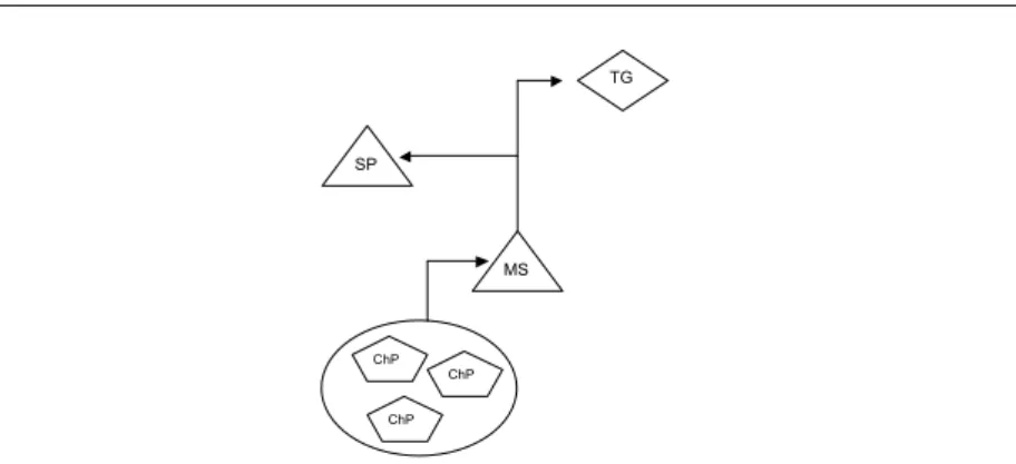
The management of these projects follow the company’s general project model called PROPS (PROfessional Project Steering). PROPS is based on the concepts of tollgates, milestones, steering points and check-points to man-age and control project deliverables. Tollgates represent long-term business decisions while milestones are predefined events representing intermediate ob-jectives at the operating work level. The monitoring of these milestones is an important element of the project management model. Steering points are de-fined to coordinate multiple parallel platform projects, e.g., handling priorities between different platform projects. The checkpoints are defined in the devel-opment process to define the work status in a process. Multiple checkpoints might have to be passed for reaching a certain milestone. Fig. 4 shows an abstract level view of these concepts.
At the operative work level, the software development is structured around work packages. These works packages are defined during the project planning
1 3 5 7 9 11 13 15 17 19 21 23 25 27 29 31 33 35 37 39 41 43 45 0 10 20 30 40 50 60 70 Weeks Fault inflow
(a) Training set.
1 2 3 4 5 6 7 8 9 10 11 12 13 14 15 5 10 15 20 25 30 35 40 45 50 Weeks Fault inflow (b) Testing set.
Fig. 3 Number of fault occurrences per week for the training set and the testing set.
phase. The work packages are defined to implement change requests or a subset of a use-case, thus the definition of work packages is driven by the functionality to be developed. An essential feature of work packages is that it allows for simultaneous work on different modules of the project at the same time by multiple teams.
Since different modules might get affected by developing a single work package, therefore it is difficult to obtain consistent metrics at the module level. The structure of a project into work packages present an obvious choice of selecting variables for the prediction models since the metrics at work package level are stable and entails a more intuitive meaning for the employees at the subject company.
Fig. 5 gives an overview of how a given project is divided into work packages that affects multiple modules. There are three sub-systems shown in Fig. 5 namely A, B and C. The division of an overall system into sub-systems is driven by design and architectural constraints. The modules belonging to the three sub-systems are named as (A1, A2), (B1, B2) and (C1, C2, C3) respectively. The overall project is divided into a number of work packages which are named
TG ChP ChP ChP MS SP
Fig. 4 PROPS concepts used in the subject company; TG, SP, MS, ChP are short for tollgate, steering point, milestone and checkpoint respectively.
in Fig. 5 as WP1, WP2,. . .,WPn. Since changes can be made to multiple modules when developing a single work package, this is shown as dashed arrow lines. The division of a project into work packages is more definitive with clear boundaries, therefore this division is shown as solid arrow lines. The Fig. 5 also show the checkpoints, steering points and the tollgates that are meant to manage and control project deliverables.
3.2 Variables selection
At our subject company the work status of various work packages is grouped using a graphical integration plan (GIP) document. The GIP maps the work packages’ status over multiple time-lines that might indicate different phases of software testing or overall project progress. There are different status rankings of the work packages, e.g., number of work packages planned to be delivered for system integration testing. A snippet of a GIP is shown in Fig. 6.
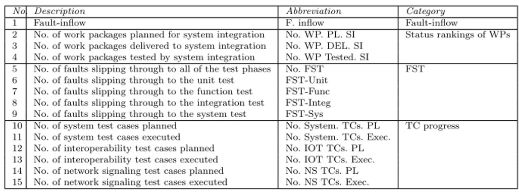
The variables of interest in this study are divided into four sets (Table 1), i.e., fault-inflow, status rankings of work packages, faults-slip-through and test case progress. A description of these four sets of variables is given below.
During the project life cycle there are certain status rankings related to the work packages (shown under the category of ‘status rankings of WPs’ in Table 1) that influence fault-inflow, i.e., the number of faults found in the consecutive project weeks. The information on these status rankings is also conveniently extracted from the GIP which is a general planning document at the company. Another important set of variables for our prediction models is the actual test case (TC) progress data, shown under the category of ‘TC progress’ in Table 1, which have a more direct influence on the fault-inflow. The information on the number of test cases planned and executed at differ-ent test phases is readily available from an automated report generation tool that uses data from an internally developed system for fault logging. These variables, along with the status rankings of the work packages, influence the
Customer requirements Project WP1 WP2 WP3 WP4 WP5 --- WPn Work packages (WPs) Sub-system A Sub-system B Sub-system C Modules Modules Modules A1 C1 C2 A2 B1 C3 B2 Time-line Checkpoints Milestones/ Steering points Tollgates Sub-system Work package Module Checkpoint Steering point Tollgate
Fig. 5 Division of requirements into work packages and modules (work model), thereby achieving tollgates, milestones/steering points and checkpoints (management model).
Table 1 Variables of interest for the prediction models.
No. Description Abbreviation Category
1 Fault-inflow F. inflow Fault-inflow
2 No. of work packages planned for system integration No. WP. PL. SI Status rankings of WPs
3 No. of work packages delivered to system integration No. WP. DEL. SI
4 No. of work packages tested by system integration No. WP Tested. SI
5 No. of faults slipping through to all of the test phases No. FST FST
6 No. of faults slipping through to the unit test FST-Unit
7 No. of faults slipping through to the function test FST-Func
8 No. of faults slipping through to the integration test FST-Integ
9 No. of faults slipping through to the system test FST-Sys
10 No. of system test cases planned No. System. TCs. PL TC progress
11 No. of system test cases executed No. System. TCs. Exec.
12 No. of interoperability test cases planned No. IOT TCs. PL
13 No. of interoperability test cases executed No. IOT TCs. Exec.
14 No. of network signaling test cases planned No. NS TCs. PL
15 No. of network signaling test cases executed No. NS TCs. Exec.
fault-inflow; so we monitor the fault-inflow as another variable for our predic-tion models. Another set of variables representing the output is the number of faults that slipped-through to the unit, function, integration and system test phases, indicated under the category ‘FST’ in Table 1. We also recorded the accumulated number of faults slipping through to all the test phases. All of
916 917 918 919 920 Work packages planned delivery to system integration Work packages delivered to system integration Work packages planned delivery to system integration Work packages post-integration tested by system integration Overall project
progress time line
System integration time line
Week 20 of year 2009
Delivered to system integration Planned delivery to system integration Post-integration tested by system integration
Fig. 6 The graphical integration plan showing the status of various work packages over multiple time-lines.
the above measurements were collected at the subject company on a weekly basis.
3.3 Test phases under consideration
Software testing is usually performed at different levels, i.e., at the level of a single module, a group of such modules or a complete system (swe, 2004). These different levels are termed as test phases in our subject company there-fore we stick to calling them test phases throughout the paper. The purpose of different test phases, as defined at our subject company, is given below:
– Unit: To find faults in module internal functional behavior e.g., memory leaks.
– Function: To find faults in functional behavior involving multiple modules. – Integration: To find configuration, merge and portability faults.
– System: To find faults in system functions, performance and concurrency. Some of these earlier test levels are composed of constituent test activities that jointly make up the higher-order test levels. The following is the division of test levels (i.e., unit, function, integration and system) into constituent activities at our subject company:
– Unit: Hardware development, module test. – Function: Function test.
– Integration: Integration of modules to functions, integration test. – System: System test, delivery test.
Our focus is then to predict the number of faults slipping through to each of these test phases.
3.4 Performance evaluation measures and prediction techniques
The evaluation of predictive performance of various techniques is done using measures of predictive accuracy and goodness of fit.
– The predictive accuracy of different techniques is compared using absolute residuals (i.e., |actual-predicted|) (Pickard et al, 1999; Kitchenham et al, 2001; Shepperd et al, 2000).
– The goodness of fit of the results from different techniques is assessed using the two-sample two-sided Kolmogorov-Smirnov (K-S) test. For the K-S test we use α = 0.05 and if the K-S statistic J is greater or equal than
the critical value Jα, we infer that the two samples did not have the same
probability distribution and hence do not represent significant goodness of fit.
We consider a technique better based on the following criteria:
– If technique A performs statistically significantly better than technique B for both predictive accuracy and goodness of fit, then technique A is declared as better.
– If no statistically significant differences are found between techniques A and B for predictive accuracy, but technique B has statistically signifi-cant goodness of fit in comparison with technique A, then technique B is declared as better.
– If no statistically significant differences are found between techniques A and B for goodness of fit, but technique B has statistically significant predictive accuracy in comparison with technique A, then technique B is declared as better.
The above mentioned evaluation procedure is an example of multi-criteria based evaluation system, a concept similar to the one presented by Lavesson et al. in (Lavesson and Davidsson, 2008).
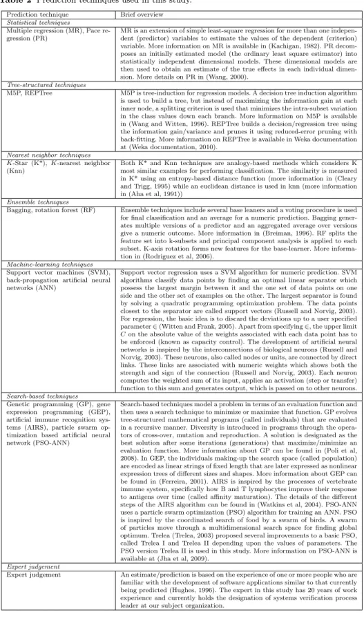
A brief description of each of the different techniques used in this study appears in Table 2. The detailed description of these techniques can be found in specific references that are given against each brief description. The techniques used can be categorized broadly into two types: prediction techniques not involving a human expert and predictions made by a human expert. There are a number of techniques that can be used for predictions that do not need a human expert. We have used established techniques (such as nearest neighbor, statistical and tree-structured techniques) as well as novel techniques that have not been used much (such as ensemble and search-based techniques).
4 Analysis and interpretation
This section describes the quantitative analysis helping us answer our research questions.
Table 2 Prediction techniques used in this study.
Prediction technique Brief overview
Statistical techniques
Multiple regression (MR), Pace re-gression (PR)
MR is an extension of simple least-square regression for more than one indepen-dent (predictor) variables to estimate the values of the depenindepen-dent (criterion) variable. More information on MR is available in (Kachigan, 1982). PR decom-poses an initially estimated model (the ordinary least square estimator) into statistically independent dimensional models. These dimensional models are then used to obtain an estimate of the true effects in each individual dimen-sion. More details on PR in (Wang, 2000).
Tree-structured techniques
M5P, REPTree M5P is tree-induction for regression models. A decision tree induction algorithm
is used to build a tree, but instead of maximizing the information gain at each inner node, a splitting criterion is used that minimizes the intra-subset variation in the class values down each branch. More information on M5P is available in (Wang and Witten, 1996). REPTree builds a decision/regression tree using the information gain/variance and prunes it using reduced-error pruning with back-fitting. More information on REPTree is available in Weka documentation at (Weka documentation, 2010).
Nearest neighbor techniques K-Star (K*), K-nearest neighbor (Knn)
Both K* and Knn techniques are analogy-based methods which considers K most similar examples for performing classification. The similarity is measured in K* using an entropy-based distance function (more information in (Cleary and Trigg, 1995) while an euclidean distance is used in knn (more information in (Aha et al, 1991))
Ensemble techniques
Bagging, rotation forest (RF) Ensemble techniques include several base leaners and a voting procedure is used
for final classification and an average for a numeric prediction. Bagging gener-ates multiple versions of a predictor and an aggregated average over versions give a numeric outcome. More information in (Breiman, 1996). RF splits the feature set into k-subsets and principal component analysis is applied to each subset. K-axis rotation forms new features for the base-learner. More informa-tion in (Rodriguez et al, 2006).
Machine-learning techniques Support vector machines (SVM), back-propagation artificial neural networks (ANN)
Support vector regression uses a SVM algorithm for numeric prediction. SVM algorithms classify data points by finding an optimal linear separator which possess the largest margin between it and the one set of data points on one side and the other set of examples on the other. The largest separator is found by solving a quadratic programming optimization problem. The data points closest to the separator are called support vectors (Russell and Norvig, 2003). For regression, the basic idea is to discard the deviations up to a user specified parameter ∈ (Witten and Frank, 2005). Apart from specifying ∈, the upper limit C on the absolute value of the weights associated with each data point has to be enforced (known as capacity control). The development of artificial neural networks is inspired by the interconnections of biological neurons (Russell and Norvig, 2003). These neurons, also called nodes or units, are connected by direct links. These links are associated with numeric weights which shows both the strength and sign of the connection (Russell and Norvig, 2003). Each neuron computes the weighted sum of its input, applies an activation (step or transfer) function to this sum and generates output, which is passed on to other neurons. Search-based techniques
Genetic programming (GP), gene expression programming (GEP), artificial immune recognition sys-tems (AIRS), particle swarm op-timization based artificial neural network (PSO-ANN)
Search-based techniques model a problem in terms of an evaluation function and then uses a search technique to minimize or maximize that function. GP evolves tree-structured mathematical programs (called individuals) that are evaluated in a recursive manner. Diversity is introduced in programs through the opera-tors of cross-over, mutation and reproduction. A solution is designated as the best solution after some iterations (generations) that maximize/minimize an evaluation function. More information about GP can be found in (Poli et al, 2008). In GEP, the individuals making-up the search space (called population) are encoded as linear strings of fixed length that are later expressed as nonlinear expression trees of different sizes and shapes. More information about GEP can be found in (Ferreira, 2001). AIRS is inspired by the processes of vertebrate immune system, specifically how B and T lymphocytes improve their response to antigens over time (called affinity maturation). The details of the different steps of the AIRS algorithm can be found in (Watkins et al, 2004). PSO-ANN uses a particle swarm optimization (PSO) algorithm for training an ANN. PSO is inspired by the coordinated search of food by a swarm of birds. A swarm of particles move through a multidimensional search space for finding global optimum. Trelea (Trelea, 2003) proposed several improvements to a basic PSO, called Trelea I and Trelea II depending upon the values of parameters. The PSO version Trelea II is used in this study. More information on PSO-ANN is available at (Jha et al, 2009).
Expert judgement
Expert judgement An estimate/prediction is based on the experience of one or more people who are
familiar with the development of software applications similar to that currently being predicted (Hughes, 1996). The expert in this study has 20 years of work experience and currently holds the designation of systems verification process leader at our subject organization.
4.1 Analyzing dependencies among variables
Before applying the specific techniques for prediction, we analyzed the depen-dencies among variables (see Table 1) using scatter plots. We were especially interested in visualizing:
– the relationship between the measures of status rankings of work packages. – the relationship between the measures of test case progress.
– fault-inflow vs. the rest of the measures related to status rankings of work packages and test case progress.
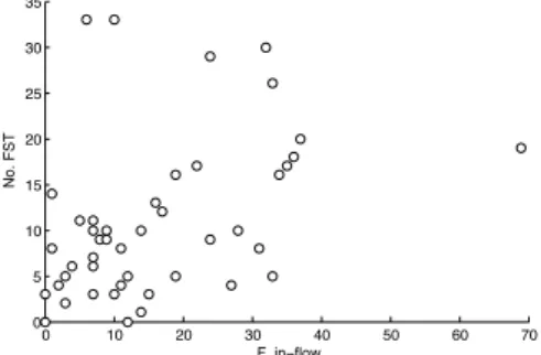
The pair-wise scatter plots of the above attributes showed a tendency of non-linear relationship. Two of these scatter plots are shown in Fig. 7 for fault-inflow vs. number of faults slipping through all of the test phases (Fig. 7(a)) and fault-inflow vs. number of work packages tested by system integration (Fig. 7(b)). 0 10 20 30 40 50 60 70 0 5 10 15 20 25 30 35 F. in−flow No. FST
(a) Scatter plot for fault-inflow vs. number of faults slipping through all of the test phases.
0 10 20 30 40 50 60 70 0 5 10 15 20 25 F. in−flow No. WP Tested. SI
(b) Scatter plot for fault-inflow vs. number of work packages tested by system integration.
Fig. 7 Example scatter plots for fault-inflow vs. number of faults slipping through all of the test phases and fault-inflow vs. number of work packages tested by system integration.
After getting a sense of the relationships among the variables, we used kernel principal component analysis (KPCA) (Canu et al, 2005) to reduce the
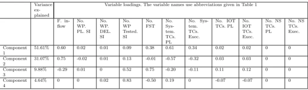
Table 3 The loadings and explained variance from four principal components. Variance
ex-plained
Variable loadings. The variable names use abbreviations given in Table 1
F. in-flow No. WP. PL. SI No. WP. DEL. SI No. WP Tested. SI No. FST No. Sys-tem. TCs. PL No. Sys-tem. TCs. Exec. No. IOT TCs. PL No. IOT TCs. Exec. No. NS TCs. PL No. NS TCs. Exec. Component 1 51.61% 0.60 0.02 0.01 0.09 0.38 0.61 0.34 0.02 0.02 0 0 Component 2 31.07% 0.75 -0.02 0.01 0.13 -0.01 -0.57 -0.32 0.03 0.03 0 0 Component 3 9.88% -0.29 0.01 0 0.52 0.75 -0.20 -0.11 0.11 0.12 0 0 Component 4 4.64% 0 0 0.02 0.83 -0.50 0.19 0 -0.07 -0.07 0 0
number of independent variables to a smaller set that would still capture the original information in terms of explained variance in the data set. The role of original variables in determining the new factors (principal components) is determined by loading factors. Variables with high loadings contribute more in explaining the variance. The results of applying the Gaussian kernel, KPCA (Table 3) showed that the first four components explained 97% of the variabil-ity in the data set. We did not include the faults-slip-through measures in the KPCA since these are the attributes we are interested in predicting. In each of the four components, all the variables contributed with different loadings, with the exception of two, namely number of network signaling test cases planned and number of network signaling test cases executed. Hence, we excluded these two variables and use the rest for predicting the faults-slip-through in different test phases.
Specifically, for predicting the faults-slippage to unit test, we use the fault-inflow, work-package status rankings and test case progress metrics. For pre-dicting the slippage to subsequent test phases we also include the slippage for the proceeding test phase; for instance when predicting the faults-slip-through at the function test phase, we also use the faults-faults-slip-through at unit test phase as an independent variable along with fault inflow, work-package status rankings and test case progress metrics.
The model training and testing procedure along with the parameter set-tings for different techniques is given in detail in Appendix A.
4.2 Performance evaluation of techniques for FST prediction
Next we present the results of the performance of different techniques in pre-dicting FST for each test phase, that would help us to answer RQ.1. As given in Section 3.4, we evaluate the prediction performance using the measures for predictive accuracy and goodness of fit.
The common analysis procedure to follow is to compare the box-plots of the absolute residuals for different prediction techniques. But since box-plots cannot confirm whether one prediction technique is significantly better than another, we use a statistical test (parametric or a non-parametric test— depending upon whether the assumptions of the test are satisfied) for testing
the equality of population medians among groups of prediction techniques. Upon the rejection of the null hypothesis of equal population medians, a mul-tiple comparisons (post-hoc) test is performed on the group medians to deter-mine which means differ. Finally, we proceed with assessing the goodness of fit using the K-S test described in Section 3.4.
4.2.1 Prediction of FST at the unit test phase
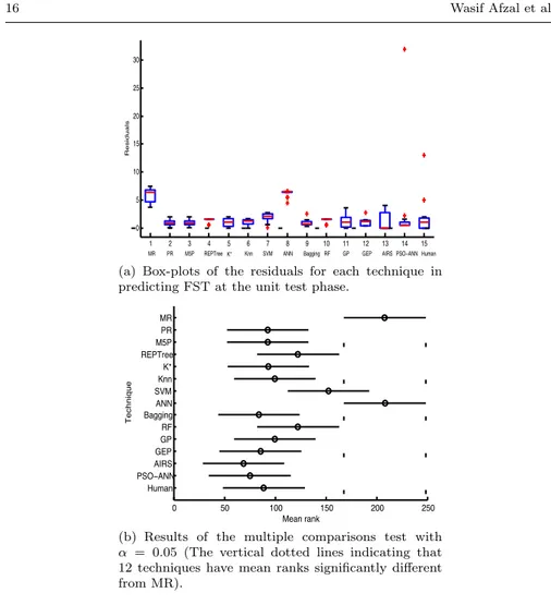
The box-plots of absolute residuals for predicting FST at the unit test phase for different techniques is shown in Fig. 8(a). The box-plot having the median value close to the 0 mark on the y-axis (shown as a dotted horizontal line in Fig. 8(a)) and a smaller spread of the distribution indicate better predictive accuracy. Keeping in view these two properties of the box-plots, there seems to be only a marginal difference in the residual box-plots of PR, M5P, Knn, Bagging, GEP and PSO-ANN. AIRS has a median at the 0 mark but shows larger spread in comparison with other techniques. The human/expert pre-diction also shows a larger spread but smaller than AIRS. Two outliers for the human prediction are extreme as compared to the one extreme outlier for PSO-ANN. Predictions from MR, SVM and ANN appear to be farther away from the 0 mark on the y-axis, an indication that the predictions are not closely matching the actual FST values.
To test for any statistically significant differences in the models’ residuals, the non-parametric Kruskal-Wallis test was used to examine any statistical differences between the residuals and to confirm the trend observed from the box-plots. The skewness in the residual box-plots for some techniques mo-tivated the use of the non-parametric test. The result of the Kruskal-Wallis
test (p = 3.2e−14) suggested that it is possible to reject the null hypothesis
of all samples being drawn from the same population at significance level, α = 0.05. This is to suggest that at least one sample median is significantly different from the others. In order to determine which pairs are significantly different, we apply a multiple comparisons test (Tuckey-Kramer, α = 0.05). The results of the multiple comparisons are displayed using a graph given in Fig. 8(b). The mean of each prediction technique is represented by a circle while the straight lines on both sides of the circle represents an interval. The means of two prediction techniques are significantly different if their intervals are disjoint and are not significantly different if their intervals overlap. For illustrative purposes, Fig. 8(b) shows vertical dotted lines for MR. There are two other techniques (SVM and ANN) where either of these two dotted lines cut through their intervals, showing that the means for MR, SVM and ANN are not significantly different. It is interesting to observe that there is only a single technique (AIRS) whose mean is significantly different (and better) than all these three techniques (i.e., MR, SVM and ANN). There are, how-ever, no significant pair-wise differences between the means of AIRS and rest of the techniques (i.e., PR, M5P, REPTree, K*, Knn, Bagging, RF, GP, GEP, PSO-ANN, Human). Human predictions, on the other hand, are significantly different and better than two of the least accurate techniques (MR, ANN).
1 2 3 4 5 6 7 8 9 10 11 12 13 14 15 0 5 10 15 20 25 30 Residuals
MR PR M5P REPTree K* Knn SVM ANN Bagging RF GP GEP AIRS PSO−ANN Human
(a) Box-plots of the residuals for each technique in predicting FST at the unit test phase.
0 50 100 150 200 250 Human PSO−ANN AIRS GEP GP RF Bagging ANN SVM Knn K* REPTree M5P PR MR Mean rank Technique
(b) Results of the multiple comparisons test with α = 0.05 (The vertical dotted lines indicating that 12 techniques have mean ranks significantly different from MR).
Fig. 8 Results showing box plots of absolute residuals and multiple comparisons of the absolute residuals between all techniques at the unit test phase.
The K-S test result for measuring the goodness of fit for predictions from each technique relative to the actual FST at the unit test phase appear in Table 4. The techniques having statistically significant goodness of fit are shown in bold (AIRS and Human). Fig. 9 shows the plot of AIRS, human and actual FST at the unit test phase. The statistically significant goodness of fit for AIRS and human can be attributed to the exact match of actual FST data on 9 out of 15 instances for AIRS and 5 out of 15 instances for the human. However, the human prediction is off by large values in the last three weeks that can also be seen as extreme outliers in Fig. 8(a).
In summary, in terms of predictive accuracy, AIRS showed significantly different absolute residuals in comparison with the three least performing tech-niques for predicting FST at the unit test phase. But then there were found no significant differences between the absolute residuals of AIRS and rest of the 11
Table 4 Two-sample two sided K-S test results for predicting FST at the unit test phase
with critical value J0.05= 0.5.
K-S test statistic, J
MR PR M5P REPTree K* Knn SVM ANN Bagging RF GP GEP AIRS PSO-ANN Human 1 0.60 0.60 0.93 0.53 0.80 0.87 1 0.80 0.93 0.53 0.80 0.27 0.73 0.33 0 1 2 3 4 5 6 7 8 9 10 11 12 13 14 15 −5 0 5 10 Weeks FST AIRS Actual human
Fig. 9 Plot of the predicted vs. the actual FST values at the unit test phase for techniques having significant goodness of fit.
techniques. Human predictions showed significantly different absolute residu-als in comparison with the two least performing techniques for predicting FST at the unit test phase. For goodness of fit, AIRS and human predictions were found to be statistically significant, though the human predictions resulted in extreme values later in the prediction period.
4.2.2 Prediction of FST at the function test phase
The box-plots of absolute residuals for predicting FST at the function test phase for different techniques is shown in Fig. 10(a). We can observe that there is a greater spread of distribution for each of the techniques as compared with those at the unit test phase. The box-plots for each of the techniques are also farther away from the 0 mark on the y-axis, with PSO-ANN and SVM having the median closet of all to the 0 mark on the y-axis. Human and MR prediction shows the greatest spread of distributions while the box-plots of PR, M5P, K*, Knn and Bagging show only a marginal difference. The result
of the Kruskal-Wallis test (p = 1.6e−11) at α = 0.05 suggested that at least
one sample median is significantly different from the others. Subsequently, the results of the multiple comparisons test (Tuckey-Kramer, α = 0.05) appear in Fig. 10(b). The absolute residuals of MR and human are not significantly different (as their intervals overlap), a confirmation of the trend observed from the box-plots. Two of the better techniques having lower medians are SVM and PSO-ANN. There are no significant differences between the two. Also there are no significant pair-wise differences between SVM and each one of: PR, M5P, REPTree, K*, Knn, Bagging, GP, GEP.
1 2 3 4 5 6 7 8 9 10 11 12 13 14 15 0 2 4 6 8 10 12 14 Residuals
MR PR M5P REPTree K* Knn SVM ANN Bagging RF GP GEP AIRS PSO−ANN Human
(a) Box-plots of the residuals for each technique in predicting FST at the function test phase.
0 50 100 150 200 250 Human PSO−ANN AIRS GEP GP RF Bagging ANN SVM Knn K* REPTree M5P PR MR Mean rank Technique
(b) Results of the multiple comparisons test with α = 0.05 (The vertical dotted lines indicating that 6 techniques have mean ranks significantly different from MR).
Fig. 10 Results showing box plots of absolute residuals and multiple comparisons of the absolute residuals between all techniques at the function test phase.
Table 5 Two-sample two sided K-S test results for predicting FST at the function test
phase with critical value J0.05= 0.5.
K-S test statistic, J
MR PR M5P REPTree K* Knn SVM ANN Bagging RF GP GEP AIRS PSO-ANN Human 1 0.93 0.93 0.73 0.93 0.93 0.4 1 0.80 0.93 0.93 0.93 0.93 0.4 0.73
The K-S test result for measuring the goodness of fit for predictions from each technique relative to the actual FST at the function test phase appear in Table 5. SVM and PSO-ANN show statistically significant goodness of fit. Fig. 11 shows the line plots of SVM and PSO-ANN with the actual FST at the function test phase. SVM appears to behave in Fig. 11 since there are no high peaks showing outliers (as is the case with PSO-ANN in Week 11).
In summary, in terms of predictive accuracy, residual box-plots indicate that SVM and PSO-ANN are better at predicting FST at the function test
0 1 2 3 4 5 6 7 8 9 10 11 12 13 14 15 −4 −2 0 2 4 6 8 10 12 14 Weeks FST PSO−ANN Actual SVM
Fig. 11 Plot of the predicted vs. the actual FST values at the function test phase for techniques having significant goodness of fit.
phase but there are no significant differences found with the majority of the other techniques. Also MR and human predictions are significantly worse than seemingly better SVM and PSO-ANN. SVM and PSO-ANN also show statis-tically significant goodness of fit in comparison with other techniques.
4.2.3 Prediction of FST at the integration test phase
The box-plots of absolute residuals for predicting FST at the integration test phase for different techniques is shown in Fig12(a). We can observe that there is a smaller spread of distribution for each technique as compared with the box-plots for function test. An exception is ANN whose box-plot is more spread out than other techniques. In terms of the median being close to the 0 mark on the y-axis, Bagging and GP appear to be promising, though there seem to be only marginal differences in comparison with PR, M5P, REPTree and PSO-ANN. GEP and human each shows two extreme outliers. The result of the
Kruskal-Wallis test (p = 1.7e−5) at α = 0.05 suggested that at least one sample
median is significantly different from the others. Subsequently, the results of the multiple comparisons test (Tuckey-Kramer, α = 0.05) appear in Fig. 12(b). The mean rank for MR is not significantly different than the ones for SVM, ANN and the human. GP has the mean rank that is significantly different than MR and ANN, the two least performing techniques. However, there are not any pair-wise significant differences between the absolute residuals for GP and each one of: PR, M5P, REPTree, K*, Knn, SVM, Bagging, RF, GEP, AIRS, PSO-ANN and Human.
The K-S test result for measuring the goodness of fit for predictions from each technique relative to the actual FST at the integration test phase appear in Table 6. Bagging, GP, AIRS and human predictions show statistically sig-nificant goodness of fit. Fig. 13 show the line plots of Bagging, GP, AIRS and the human predictions.
1 2 3 4 5 6 7 8 9 10 11 12 13 14 15 0 5 10 15 20 25 30 35 40 Residuals
MR PR M5P REPTree K* Knn SVM ANN Bagging RF GP GEP AIRS PSO−ANN Human
(a) Box-plots of the residuals for each technique in predicting FST at the integration test phase.
0 50 100 150 200 250 Human PSO−ANN AIRS GEP GP RF Bagging ANN SVM Knn K* REPTree M5P PR MR Technique Mean rank
(b) Results of the multiple comparisons test with α = 0.05 (The vertical dotted lines indicating that eleven techniques have mean ranks significantly differ-ent from MR).
Fig. 12 Results showing box plots of absolute residuals and multiple comparisons of the absolute residuals between all techniques at the integration test phase.
Table 6 Two-sample two sided K-S test results for predicting FST at the integration test
phase with critical value J0.05= 0.5.
K-S test statistic, J
MR PR M5P REPTree K* Knn SVM ANN Bagging RF GP GEP AIRS PSO-ANN Human 0.73 0.60 0.60 0.60 0.60 0.60 0.60 0.60 0.40 0.60 0.33 0.60 0.27 0.60 0.27
In summary, in terms of predictive accuracy, MR and ANN appear to be the two least performing techniques for predicting FST at the integration test phase, while there were no statistically significant differences between the majority of the techniques. Bagging, GP, AIRS and human predictions show statistically significant goodness of fit in comparison with other techniques.
0 1 2 3 4 5 6 7 8 9 10 11 12 13 14 15 −2 −1 0 1 2 3 4 5 6 Weeks FST AIRS Actual Bagging
(a) Plot of the actual vs. predicted FST values (AIRS and Bagging) at the integration test phase.
0 1 2 3 4 5 6 7 8 9 10 11 12 13 14 15 −2 −1 0 1 2 3 4 5 6 7 8 9 Weeks FST Actual Human GP
(b) Plot of the actual vs. predicted FST values (Hu-man and GP) at the integration test phase.
Fig. 13 Plot of the predicted vs. the actual FST values at the integration test phase for techniques having significant goodness of fit.
4.2.4 Prediction of FST at the system test phase
The box-plots of absolute residuals for predicting FST at the system test phase for different techniques is shown in Fig. 14(a). We can observe that there are certain techniques that appear to do better. These are PR, RF and GP. The box-plots of these three techniques have medians closer to the 0 mark on the y-axis, with GP being the closest. GP also show the smallest distribution as compared with PR and RF. For the rest of the techniques, there is a greater variance in their plots with outliers. MR, Knn, AIRS and human box-plots seem to be worse, both in terms of the position of the median and the
spread of the distribution. The result of the Kruskal-Wallis test (p = 5.6e−7)
at α = 0.05 suggested that at least one sample median is significantly different from the others. Subsequently, the results of the multiple comparisons test (Tuckey-Kramer, α = 0.05) appear in Fig. 14(b). The technique with smallest mean rank is GP and there are no pair-wise significant differences between GP
1 2 3 4 5 6 7 8 9 10 11 12 13 14 15 0 5 10 15 Residuals
MR PR M5P REPTree K* Knn SVM ANN Bagging RF GP GEP AIRS PSO−ANN Human
(a) Box-plots of the residuals for each technique in predicting FST at the system test phase.
−50 0 50 100 150 200 250 Human PSO−ANN AIRS GEP GP RF Bagging ANN SVM Knn K* REPTree M5P PR MR Mean rank Technique
(b) Results of the multiple comparisons test with α = 0.05 (The vertical dotted lines indicating that 3 techniques have mean ranks significantly different from MR).
Fig. 14 Results showing box plots of absolute residuals and multiple comparisons of the absolute residuals between all techniques at the system test phase.
and any of the techniques: PR, Bagging, RF and PSO-ANN. This finding also confirms the trend from the box-plots. MR is the worst performing technique and there are no pair-wise significant differences between MR and any of the techniques: M5P, REPTree, K*, Knn, SVM, ANN, Bagging, GEP, AIRS, PSO-ANN and Human.
The K-S test result for measuring the goodness of fit for predictions from each technique relative to the actual FST at the system test phase appear in Table 7. PR, GP and PSO-ANN show statistically significant goodness of fit. Fig. 15 shows the line plots of PR, GP, PSO-ANN with the actual FST at the system test phase.
In summary, in terms of predictive accuracy, GP, PR, Bagging, RF and PSO-ANN perform better than the other techniques for predicting FST at
Table 7 Two-sample two sided K-S test results for predicting FST at the system test phase
with critical value J0.05= 0.5.
K-S test statistic, J
MR PR M5P REPTree K* Knn SVM ANN Bagging RF GP GEP AIRS PSO-ANN Human 0.67 0.40 0.73 0.93 0.93 0.80 0.87 0.47 0.93 0.67 0.20 0.80 0.73 0.40 0.60 0 1 2 3 4 5 6 7 8 9 10 11 12 13 14 15 −2 0 2 4 6 8 10 12 14 Weeks FST PSO−ANN Actual
(a) Plot of the actual vs. predicted FST values (PSO-ANN) at the system test phase.
0 1 2 3 4 5 6 7 8 9 10 11 12 13 14 15 −2 0 2 4 6 8 10 12 14 Weeks FST Actual GP PR
(b) Plot of the actual vs. predicted FST values (GP and PR) at the system test phase.
Fig. 15 Plot of the predicted vs. the actual FST values at the system test phase for tech-niques having significant goodness of fit.
the system test phase. PR, GP and PSO-ANN show statistically significant goodness of fit in comparison with other techniques.
4.3 Performance evaluation of human expert judgement vs. other techniques for FST prediction
The analysis done in the previous Section 4.2 would also allow us to answer the RQ.2 that questions if other techniques better predict FST than human expert
judgement. We now analyze the performance of human expert judgement vs. other techniques for FST prediction at each of the four test phases.
4.3.1 Prediction of FST at the unit test phase
Fig. 8(b) shows the results of the multiple comparisons test (Tuckey-Kramer, α = 0.05) for FST prediction at the unit test phase. Two techniques have their means significantly different (and worse) than the human expert judgement. These techniques are MR and ANN. Otherwise, there are no significant pair-wise differences between the means of human expert judgement and rest of the techniques.
In terms of goodness of fit, Table 4 shows that AIRS and human expert judgement have statistically significant goodness of fit in comparison with other techniques.
4.3.2 Prediction of FST at the function test phase
Fig. 10(b) shows the results of the multiple comparisons test (Tuckey-Kramer, α = 0.05) for FST prediction at the function test phase. Three techniques have their means significantly different (and better) than the human expert judgement. These techniques are PSO-ANN, SVM and Knn. Otherwise, there are no significant pair-wise differences between the means of human expert judgement and the rest of the techniques.
In terms of goodness of fit, Table 5 shows that human expert judgement have no significant goodness of fit in comparison with SVM and PSO-ANN. 4.3.3 Prediction of FST at the integration test phase
Fig. 12(b) shows the results of the multiple comparisons test (Tuckey-Kramer, α = 0.05) for FST prediction at the integration test phase. No technique has its mean significantly different than the human expert judgement.
In terms of goodness of fit, Table 6 shows that Bagging, GP, AIRS and human expert judgement have significant goodness of fit in comparison with rest of the techniques.
4.3.4 Prediction of FST at the system test phase
Fig. 14(b) shows the results of the multiple comparisons test (Tuckey-Kramer, α = 0.05) for FST prediction at the system test phase. GP has its mean significantly different (and better) than the human expert judgement.
In terms of goodness of fit, Table 7 shows that GP and PSO-ANN have significant goodness of fit in comparison with rest of the techniques.
Table 8 sums up which techniques are or are not better than human expert judgement in predicting FST at unit, function, integration and system test phases. The dark grey cells in the Table 8 refers to techniques that are equally good in predicting FST with the human expert judgement. The light grey cells
Table 8 A summary of techniques that are or are not better than human experts predicting FST at unit, function, integration and system test phases.
Human expert judgement vs.
MR PR M5P REPTree K* Knn SVM ANN Bagging RF GP GEP AIRS PSO-ANN Unit
Function Integration
System
indicate that the techniques are inferior with respect to the human judgement and the dark grey cells. The white cells indicate that these techniques are better than human expert judgement in predicting FST.
5 Discussion
One of the basic objectives of doing measurements is monitoring of activities so that action can be taken as early as possible to control the final outcome. With this objective in focus, FST metrics work towards the goal of minimization of avoidable rework by finding faults where they are most cost-effective to find. Early prediction of FST at different test phases is an important decision support to the development team whereby advance notification of improvement potential can be made.
In this paper we investigated two research questions outlined in Section 1. RQ.1 investigated the use of a variety of techniques for predicting FST in unit, function, integration and system test phases. The results are evaluated for predictive accuracy (through absolute residuals) and goodness of fit (through the Kolmogorov-Smirnov test). A range of techniques are found to be useful in predicting FST for different test phases (both in terms of predictive accuracy and goodness of fit). RQ.2 is concerning a more specific research question that compared human expert judgement with other techniques. The results of this comparison indicate that expert human judgement is better than majority of the techniques at unit and integration test but are far off at function and system test. Hence, human predictions regarding FST lack some consistency. There are indications that a smaller group of techniques might be consistently better in predicting at all the test phases. Following is the list of techniques performing better at various test phases for predicting FST in our study:
1. Unit test – AIRS and human. 2. Function test – SVM and PSO-ANN.
3. Integration test – Bagging, GP, AIRS, human. 4. System test – PR, GP, PSO-ANN.
A trend that can be observed from this list of comparatively better techniques is that there is a representation of search-based techniques in predicting FST at each test phase.
– AIRS is consistently better at – Unit and integration test. – PSO-ANN is consistently better at – function and system test
– GP is consistently better at – integration and system test.
The search-based techniques have certain merits, one or more of which might be responsible for outperforming the other group of techniques:
– The search-based techniques are better able to cope with ill-defined, partial and messy input data (Harman, 2010). GP is able to perform well where the interrelationships among the relevant variables are unknown or poorly understood (Poli et al, 2008). According to Poli et al. (Poli et al, 2008), “[GP] has proved successful where the appli- cation is new or otherwise not well understood. It can help discover which variables and operations are important; provide novel solutions to individual problems; unveil un-expected relationships among variables; and, sometimes GP can discover new concepts that can then be applied in a wide variety of circumstances.” Evolutionary algorithms have also been applied successfully to problems where there are high correlations between variables, i.e, the choice of one variable may change the meaning or quality of another (Blickle, 1996). – GP is particularly good at providing small programs that are nearly correct
and predictive models are not exceptionally long (Harman, 2010). Accord-ing to Poli et al. (Poli et al, 2008),“[. . .] evolutionary algorithms tend to work best in domains where close approximations are both possible and ac-ceptable.” Search-based techniques can produce very transparent solutions, in the sense that they can make explicit the weight and contribution of each variable in the resulting solutions.
– Being non-parametric approaches, the structure of the end solution is not pre-conceived. This is particularly important for the usability of search-based techniques, i.e., the techniques used for prediction should be able to determine the form of relationship between inputs and outputs rather than that the technique is dependent on the user providing the form of the relationship.
– Search-based techniques are entirely data driven approaches and do not include any assumptions about the distribution of the data in its formula-tion. For example, GP models are independent of any assumptions about the stochastic behavior of the software failure process and the nature of software faults (Afzal, 2009).
The results also argue that there is value in the use of other techniques like human predictions, SVM, Bagging and PR, it is just that these are not as consistent as the search-based techniques.
Another interesting outcome of this study is the performance of search-based techniques (and other better performing techniques) outside their re-spective training ranges, i.e., the predictions are evaluated for 15 weeks of an on-going project after being trained on another baseline project data. This is to say that the over-fitting is within acceptable limits, and this is particularly encouraging considering the fact that we are dealing with large projects where the degree of variability in fault occurrences can be large. This issue is also related to the amount of data available for training the different techniques which, in case of large projects, is typically available.
Another important aspect of the results is that human predictions were among the better techniques for predicting FST at unit and integration test. In our view, this is also an important outcome and shows that expert opinions perhaps need more consideration that is largely been ignored in empirical studies of software fault predictions (Tomaszewski et al, 2007; Catal and Diri, 2009). We, therefore, agree with the conclusion of Hughes (Hughes, 1996) that expert judgement should be supported by the use of other techniques rather than displacing it. Search-based techniques seem to be an ideal decision-support tool for two reasons:
1. They have performed consistently better than other techniques (Section 4.2). 2. Search-based techniques, as part of the more general field of search-based
software engineering (SBSE) (Harman and Jones, 2001; Harman, 2007), is inherently concerned with improving not with proving (Harman, 2010).
As such it is likely that human-guided semi-automated search might help get a reasonable solution that incorporates human judgement in the search process. This human-guided search is commonly referred to as ‘human-in-the-loop’ or ‘interactive evolution’ (Harman, 2010) and is a promising area of future re-search. The incorporation of human feedback in the automated search can possibly account for some of the extreme fluctuations in the solely human predictions that are observed for predicting FST at unit and integration test. We also believe that the selection of predictor variables that are easy to gather (e.g., the project level metrics at the subject company in this study) and that do not conflict with the development life cycle have better chances of industry acceptance. There is evidence to support that general process level metrics are more accurate than code/structural metrics (Arisholm et al, 2010). A recent study by Afzal (Afzal, 2010) has shown that the use of number of faults-slip-through to/from various test phases are able to provide good results for finding fault-prone modules at integration and system test phases. However this subject requires further research.
We have also come to realize that the calculation of simple residuals and goodness of fit tests along with statistical testing procedures are a sound way to secure empirical findings where the outcome of interest is numeric rather than binary. An assessment of the qualitative features can then be undertaken as an industrial survey to complement the initial empirical findings.
While working on-site at the subject organization for this research, we realized several organizational factors that influence the success of such a decision-support. Managerial support and an established organizational cul-ture of quantitative decision-making allowed us to gain easy access to data repositories and relevant documentation. Moreover, collection of faults-slip-through data and association of that data to modules, was made possible using automated tool support that greatly reduced the time for data collection and ensured data integrity.
6 Empirical validity evaluation
We adopted a case study approach in evaluating various techniques for predict-ing FST in four test phases. A controlled experiment was deemed not practical since too many human factors potentially affect fault occurrences.
What follows next is our presentation of the various threats to validity of our study: Construct validity. Our choice of selecting project level metrics (Table 1) instead of structural code metrics was influenced by multiple factors. First, metrics relevant to work packages (Section 3.1) have an intuitive appeal for the employees at the subject company where they can relate FST to the proportion of effort invested. Secondly, the existence of a module in multiple work packages made it difficult to obtain consistent metrics at the component level. Thirdly, the intent of this study is to use project level metrics that are readily available and hence reduces the cost of doing such predictions. In addi-tion, the case study is performed in the same development organization having the identical application domain, so the two projects in focus are characterized by the same set of metrics. Internal validity. A potential threat to the internal validity is that the FST data did not consider the severity level of faults, rather treated all faults equally. As for the prediction techniques, the best we could do was to experiment with a variety of parameter values. But we acknowl-edge that the obtained results could be improved by better optimizing the parameters. External validity. The quantitative data modeling was performed on data from a specific company while the questionnaire was filled out by an expert having 20 years of work experience and currently holds the designation of systems verification process leader at our subject organization. The ques-tionnaire was filled to provide expert estimations of FST metric and consisted of all relevant independent variables. The expert then used these independent variables to provide estimated values. In order to reduce bias arising from the design of the questionnaire, the researchers encouraged the expert for asking questions to clarify any ambiguities. We have tried to present the context and the processes to the extent possible for fellow researchers to generalize our results. We are also encouraged by the fact that the companies are enterprise-size and have development centers world-wide that follow similar practices. It is therefore likely that the results of this study are useful for them too. A threat to the external validity is that we cannot publicize our industrial data sets due to proprietary concerns. However, the transformed representation of the data can be made available if requested. Conclusion validity. We were con-scious in using the right statistical test, basing our selection on whether the assumptions of the test were met or not. We used a significance level of 0.05, which is a commonly used significance level for hypothesis testing (Juristo and Moreno, 2001); however, facing some criticism lately (Ioannidis, 2005).
7 Conclusion
In this paper, we have presented an extensive empirical evaluation of various techniques for predicting the number of faults slipping through to the four test phases of unit, function, integration and system.
We find that a range of techniques are found to be useful in such a predic-tion task, both in terms of predictive accuracy and goodness of fit. However, the group of search-based techniques (genetic programming (GP), gene ex-pression programming (GEP), artificial immune recognition system (AIRS) and particle swarm optimization based artificial neural network (PSO-ANN)) consistently give better predictions, having a representation at all of the test phases. Human predictions are also among the better techniques at two of the four test phases. We conclude that human predictions can be supported well by the use of search-based techniques and a mix of the two approaches has the potential to provide improved results.
It is important to highlight that there might be additional evaluation cri-teria that are important in addition to measuring the predictive accuracy and the goodness of fit. A general multi-criteria based evaluation system is then required that captures both the quantitative and the qualitative aspects of such a prediction task. Future work will also investigate ways to incorporate human judgement in the automated search mechanism.
There are some lessons learnt at the end of this study which might be useful for decision-making in real-world industrial projects:
– The number of faults slipping through to various test phases can be de-creased if improvement measures are taken in advance. To achieve this, prediction of FST is an important decision-making tool.
– In large industrial projects, prediction of FST is possible using project-level measurements such as fault-inflow, status ranking of work packages and test case progress.
– The organization wanting to improve their software testing process need to institutionalize a mechanism for recording data in a consistently correct manner.
– A tool support that uses the recorded data and applies a number of tech-niques to provide results to the software engineer will improve usability of any prediction effort, including FST prediction.
– A tool support is also necessary to hide complex implementation details of techniques and to ease parameter settings for end users.
– The software engineers need to be trained in the prediction task. Training workshops need to be conducted which will not only increase awareness about the potential benefits of FST prediction but will also help to discover potentially new independent variables of interest.