https://doi.org/10.1007/s00107-020-01566-1
ORIGINAL ARTICLE
Creep in oak material from the Vasa ship: verification of linear
viscoelasticity and identification of stress thresholds
R. Afshar1 · M. Cheylan2 · G. Almkvist3 · A. Ahlgren4 · E. K. Gamstedt1
Received: 16 December 2019 © The Author(s) 2020 Abstract
Creep deformation is a general problem for large wooden structures, and in particular for shipwrecks in museums. In this study, experimental creep data on the wooden cubic samples from the Vasa ship have been analysed to confirm the linearity of the viscoelastic response in the directions where creep was detectable (T and R directions). Isochronous stress–strain curves were derived for relevant uniaxial compressive stresses within reasonable time spans. These curves and the associ-ated creep compliance values justify that it is reasonable to assume a linear viscoelastic behaviour within the tested ranges, given the high degree of general variability. Furthermore, the creep curves were fitted with a one-dimensional standard linear solid model, and although the rheological parameters show a fair amount of scatter, they are candidates as input parameters in a numerical model to predict creep deformations. The isochronous stress–strain relationships were used to define a creep threshold stress below which only negligible creep is expected. These thresholds ranges were 0.3–0.5 MPa in the R direction and 0.05–0.2 MPa in the T direction.
1 Introduction
The creep properties of conserved archaeological wood material in large artefacts have not been much investi-gated despite the importance for the dimensional stability and long-term preservation. For example, the Vasa ship in Stockholm, the Bremer Cog in Bremerhaven, Mary Rose and
HMS victory in Portsmouth and the Oseberg viking ship in
Oslo, are all carrying substantial loads with different types of support structures which are aimed to minimize stresses in the hull (Jones et al. 1986; Cederlund and Hocker 2007; Hoffmann 2009). However, long-term effects from creep strains have not been explicitly taken into consideration in these support constructions. In the case of the Vasa ship,
increasing deformation of joints and load carrying mem-bers have been observed. This is to a considerable extent due to softening effect from polyethylene glycol (PEG) used as an impregnation agent to mitigate shrinkage on drying the waterlogged wood (Hocker et al. 2012; van Dijk et al.
2016). In addition, partial degradation of wood polysac-charides in the PEG-free interior of the beams is known to affect the mechanical properties (Bjurhager et al. 2012). Therefore, and as a result of planning a new support system for the Vasa, the need for more detailed information on the mechanical properties and in particular on the creep behav-iour has been identified. Previous studies have shown that the main effects of PEG on the Vasa oak compared to recent oak are increased mass density, increased hygroscopicity of the dried material (for low molecular weight PEG) and material softening. This is because PEG acts as a plasticiser (Hoffmann 2013) and reservoir of water in the PEG-rich outer layers of the wood. Therefore, variable ambient con-ditions may have a high impact on moisture content and variation in mass (Vorobyev et al. 2019), with effects on creep behaviour. Nonetheless, museums tend to showcase their ships in controlled climate (e.g., Hocker 2010), or at least with smaller moisture and temperature variations than in regular buildings. As first approximation, the creep behav-iour can be assumed to be an effect of load and time only, neglecting mechanosorptive effects due to a varying climate.
* R. Afshar
reza.afshar@angstrom.uu.se
1 Division of Applied Mechanics, The Department
of Engineering Sciences, Uppsala University, Uppsala, Sweden
2 École Nationale Supérieure de Mécanique et des
Microtechniques, Besançon, France
3 Department of Molecular Sciences, Swedish University
of Agricultural Sciences, Uppsala, Sweden
4 The Swedish National Maritime and Transport Museums,
In addressing creep of PEG-treated waterlogged wood in large wooden structures, like shipwrecks, some key ques-tions present themselves. Do these materials show linear creep within the stress levels anticipated in the structure? In a finite element model of the ship, which can potentially be used in the design of improved support structures, one would like to implement a relatively simple material model accounting for creep. This would imply a linear viscoe-lastic model accounting for creep deformation, where the creep strains depend linearly on the applied stresses within a given range. A second question to address with regard to a lower limit of this range can be formulated: Is there a stress threshold below which no creep is expected of any practi-cal importance? If such a threshold exists, it could serve as target in the design of a support structure. If the support structure can be designed in such a way that the stresses in main load carrying components are relieved down to a level beyond this threshold, creep deformation would effectively not be an issue.
In this study, experimental creep data from a first set of samples from the Vasa have been analysed. The aim was to investigate the linearity of the isochronous stress–strain curves of the creep data as well as to find the viscoelas-tic parameters and a stress threshold of the samples under creep. The tests were performed at constant climate condi-tions under three different stress levels for each of the three orthogonal directions of the wooden samples. The standard linear solid (SLS) model was used to describe the material behaviour in one loading direction at a time. The viscoelas-tic material parameters are important for characterization of the Vasa oak as well as using them in a full-scale numerical model to simulate the actual stresses on the Vasa ship and understand its creep behavior. The approach is considered applicable also to other large wooden structures, specifically PEG-treated waterlogged wooden shipwrecks.
2 Experimental procedures
The experimental tests were performed in a room with controlled climate such that the relative humidity (RH) was 54 ± 1% and temperature was 20 ± 0.1 °C. Eight cubic samples of the Vasa oak of various origins in the ship pre-pared for testing in the three orthogonal directions, i.e., longitudinal (L), radial (R) and tangential (T), are pre-sented in Table 1. The dimension of the cubic samples was 11 × 11 × 11 mm3. Since mechanical testing is destructive
and the material is very precious, only small samples could be spared for mechanical characterization. These were taken primarily from drill cores left when ventilation holes were installed. Although the small specimens mean a larger material variability, one advantage was that the curvature of the annual rings was large compared to the specimen
dimensions. The samples could therefore be regarded as orthotropic in a Cartesian sense rather than polar ortho-tropic, which facilitates a direct identification of the mechan-ical properties from uniaxial testing along the material axes (Shipsha and Berglund 2007). Two samples were loaded in R direction, four in T direction, and two in L direction. All tests were performed in compression, as this is more com-mon than tension in large structures, where the loads come from the self-weight. The creep deformation was monitored at three stress levels in different orthogonal directions for different samples. According to earlier studies on Vasa wood the longitudinal strength is significantly decreased due to cellulose depolymerisation (Bjurhager et al. 2012). Therefore, more conservative stress levels were chosen in L direction compared to R and T direction. For each sample a camera recorded the deformation with an interval of every 2 s until 100 s, and then every thirty minutes until the end of each period at each stress level. The stress levels were maintained for about fifty days resulting in a total experi-mental time of 4 months, as shown in Fig. 1. For the sake of traceability, the sample IDs are the same as the unambiguous identification numbers used by the museum.
After recording a series of photographs from one side of each sample, image analysis from software GOM Aramis
Table 1 Vasa oak samples used in the experiment
Loading direction Stress levels (MPa) Sample ID Sample site Radial (R) 0.8, 1.2 and 1.6 65901-09 Hole: beam 65903-07 Hole: stringer Tangential (T) 0.4, 0.6 and 0.8 65905-01 Keel
65904-06 Keel 65900-01 Hole: beam 65901-11 Hole: beam Longitudinal (L) 1.2, 1.8 and 2.4 65900-11 Hole: beam 65902-04 Hole: stringer
Fig. 1 Experimental set-up for the creep testing: L1 is 70 cm and L2 is
stereo system 5 M (Braunschweig, Germany) was used to obtain the average strain of the samples at every time interval. The measurements of the side of the sample were expressed in two perpendicular strains (𝜀y and 𝜀x ). Since
the purpose of the present study is only to investigate creep linearity and the presence of the creep threshold, we confine ourselves to a one-dimensional case, where only 𝜀y was used,
as it represents the strain in the loading direction. Later, the strain curves perpendicular to loading direction ( 𝜀x ) and
corresponding Poisson ratio (υxy) calculations are used to
identify an orthogonal 3D creep model, which can be imple-mented for solid-shell elements in a finite element model.
3 Materials and methods
3.1 Material model
The following procedure describes the method to obtain the viscoelastic material parameters (hereinafter referred to as material parameters, unless otherwise stated) in loading direction only.
In this study, the material model is chosen as a linear viscoelastic model called standard linear solid (SLS) (Ward and Sweeney 2004). This is one of the simplest creep mod-els, which qualitatively shows the same behaviour as that observed in experiments. The trend of this model consists of an initial elastic deformation followed by decelerating creep deformation slowly approaching an asymptotic strain level for extended periods of testing time. The SLS model has two configurations, which depend on the connection of spring and damper. If spring and damper are in series, it yields a Maxwell model, while connecting a spring and damper in parallel yields a Kelvin–Voigt model of a material. Here, the Maxwell configuration is used. The Kelvin–Voigt configura-tion is adopted in the paper by Huč and Svensson (2018).
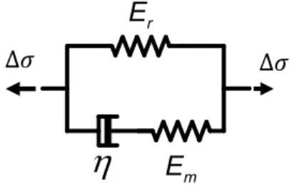
According to linear viscoelastic theory, the relaxation and creep functions are only a function of time, which means that behaviour of the material is independent of strain or stress. The SLS model is a three-parameter model (Er, Em, and τ) that contains a Maxwell arm in parallel with an elastic arm as shown in Fig. 2.
In Fig. 2, Er and Em are the spring parameters of the
elas-tic arm and Maxwell arm, respectively and η is the viscous parameter of the dashpot in Maxwell arm.
The governing equation, obtained in time domain, where strain is a function of applied stress, Δ𝜎 , and creep compli-ance modulus J (t) is given by
(1) 𝜀(t) = Δ𝜎 ( 1 Er+ Em + ( 1 Er − 1 Er+ Em )( 1− e− Er Em 𝜂(Er +Em)t )) = Δ𝜎J(t)
The creep compliance modulus is simplified as follows
where the glassy compliance (Cg), which is the value of
creep compliance when the material exhibits glassy behaviour at the beginning of the creep test, the rubbery compliance (Cr) the value of creep compliance at rubbery stage of the mate-rial and the characteristic time 𝜏c are given in the following
expressions:
The creep model in Eq. (1) in combination with the curve fitting tool in Matlab was used to identify the two viscoelastic parameters of SLS model from the experimental creep data, namely as relative modulus α and relaxation time τ. The for-mer, α, is the relative stiffness loss at infinite time, and the latter, τ, is the time related to the decay rate and defined as the ratio of viscosity (η) to the spring constant of Maxwell arm ( Em ). To calculate α and τ, first Cg, Cr and τc were obtained
through fitting Eq. (2) to experimental data. Note that Eq. (2) is a simplified version of Eq. (1). After that, Er and Em were obtained using Eqs. (3) and (4). Finally, the parameters α and
τ are defined as follows:
According to Boltzmann superposition principle (e.g.,Ward and Sweeney 2004), as depicted in Fig. 3, at time
t1, stress Δσ1 is applied and induced strain is given by
(2) J(t) =𝜀(t) Δ𝜎 =(Cg+(Cr− Cg)(1 − e −t∕𝜏c)) (3) Cg= 1 Er+ Em (4) Cr= 1 Er (5) 𝜏c= Cr Cg𝜏 (6) 𝛼= Em Er+ Em (7) 𝜏= 𝜏c Cr∕Cm .
According to linear viscoelasticity, the compliance J(t) is independent of stress, i.e. it is the same for all the stresses at a specific time. If stress increment Δσ2 is applied at time
t2, then the strain increase due to stress increment Δσ2 can
be given by
Finally, the strain increase due to Δσ3 can be written as follows
4 Results and discussion
In this section, before presenting the viscoelastic parameters for all of the samples, the viscoelastic parameter extraction for a sample curve, verification of linear viscoelasticity according to Boltzmann principle as well as stress threshold identification are demonstrated.
4.1 Viscoelastic parameters extraction
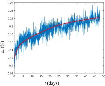
In Fig. 4, the strain curve and curve fitting of sample 65901-11 at the first stress level (Δσ = 0.4 MPa) in the T direc-tion are shown. Some transients were observed during load increase followed by a period for the sample to settle in. Therefore, the first three hours of the experimental data were excluded from the curve fitting procedure. The correspond-ing results, in terms of α and τ for all eight samples are presented in the results section below.
(8) 𝜀1(t) = Δ𝜎1J(t) (9) 𝜀2(t) = Δ𝜎2J(t − t2 ) (10) 𝜀3(t) = Δ𝜎3J(t − t3 )
4.2 Verification of linear viscoelasticity and identification of a creep threshold
It is well known that the theory of linear viscoelasticity is valid for the low stress levels, which is the condition of this study. As exemplified by sample 65901-11 (T direction), the linearity of the SLS model is demonstrated by the three stress increments Δσi = 0.4, 0.2 and 0.2 MPa, for i = 1, 2
and 3, respectively. The creep response is shown in Fig. 5, where the effects of step-wise adding of the stress can be clearly observed.
To plot the isochronous stress–strain curves at each point in time, the strain values were taken from the creep curves
Δσ1 Δσ2 Δσ3 σ ε t t t1 t2 t3
Fig. 3 Creep behaviour of linear viscoelastic solid according to Boltzmann principle 0 5 10 15 20 25 30 35 40 45 50 0.08 0.1 0.12 0.14 0.16 0.18 0.2 0.22 0.24 0.26 εy (%) t (days)
Fig. 4 Example of curve fitting to identify the creep parameters from strain in loading direction (T) of sample 65901-11
0 50 100 150 0 0.1 0.2 0.3 0.4 0.5 0.6 t (days) εy (%) Sample 65901-11
Fig. 5 Strain as a function of time under three stress increments for sample 65901-11 loaded in the T direction
that were also taken at specific moments in time at differ-ent stress level, as shown in Fig. 6. Each stress level can be obtained by adding the previous stress increments. For example, the second stress level for samples in T-direction is σ2 = Δσ1 + Δσ2 = 0.4 + 0.2 MPa = 0.6 MPa. In addition, notice that for a different orthogonal direction, different stress increment was used to cover stress ranges considered relevant for the various directions (cf. Table 1). Usually, the measured strain has large fluctuations. Therefore, to extract the stress and strain at different time points the measured curve needs to be smoothed. Smoothing is a method of reducing the noise within a data set. Different methods such as moving average, Savitzky–Golay filters, and local regres-sion with and without weights and robustness can be used. In this work, the RLOESS (locally weighted non-parametric regression fitting using a 2nd order polynomial) function in Matlab with the span of 0.5 was used to plot the strain as a function of time at different stress levels (Fig. 6). The span is the number of data points for calculating the smoothed value, specified as an integer or as a scalar value in the range (0,1) denoting a fraction of the total number of data points.
By extracting the stress and strain at different time points (t1, t2 and t3 in Fig. 6) and connecting the data points, it is
possible to plot the stress–strain relationship, as shown in Fig. 7. Contrary to conventional stress–strain diagrams, it was chosen to present the data with stress along the abscissa and strain along the ordinate, since the creep compliance is then defined by the slope in the diagram. The data from Fig. 7 and the corresponding compliance moduli for each stress level are also given in Table 2. Due to limitations in time and the scarcity of material, samples sufficient to only
3 stress levels could be spared. Some material was saved by increasing the stress level in a step-wise manner for each sample. It is however then assumed that the previous load-ing steps do not affect the creep behaviour of the subsequent ones.
According to linear viscoelasticity, the compliance J(t) should be independent of stress, i.e. it is the same for all the stress levels at a particular point in time. Considering the large variation in properties in general for these materials, the relatively small variation in J in Table 2 confirms this hypothesis of linear viscoelasticity for practical purposes within the chosen range of stresses and time.
In addition to independence of creep compliance J with respect to stress level σ, presented in Table 2, the linearity can also be confirmed by the similarity of the isochronous stress–strain curves in Fig. 7.
Normally, a stress threshold in creep is defined by the stress level below which the creep rate, dε/dt, is zero (e.g., Zhang 2010). The limited creep data for the archaeologi-cal material does not allow characterization of this type of threshold. Instead, the isochronous stress–strain data were considered, which in the present case take a convex shape including the certain data point in the origin (no stress, no creep strain) in the ε–σ plot. If data points are extrapolated down to the intersection with the stress axis or x-axis, a creep threshold stress can be defined, as schematically shown in Fig. 7. Below this stress value, only negligible creep is expected. If a support structure could be designed to relieve stresses in the wooden artefact down to this level, creep could in principle be ignored.
No creep was detected in the samples loaded in lon-gitudinal direction (Vorobyev et al. 2019). The main reason can be that the samples were loaded under the stress threshold in L direction. In addition, this could be understood from a composite mechanics perspective. In the L direction, the cellulose microfibrils carry most
0 10 20 30 40 50 60 time (days) 0 0.1 0.2 0.3 0.4 0.5 0.6
t
1σ
1σ
2σ
3t
2t
3 t (days) εy (%) Sample 65901-11Fig. 6 Strain as a function of time at different stress levels for sample 65901-11 loaded in the T direction. The indicated times were chosen to establish the isochronous stress–strain relations
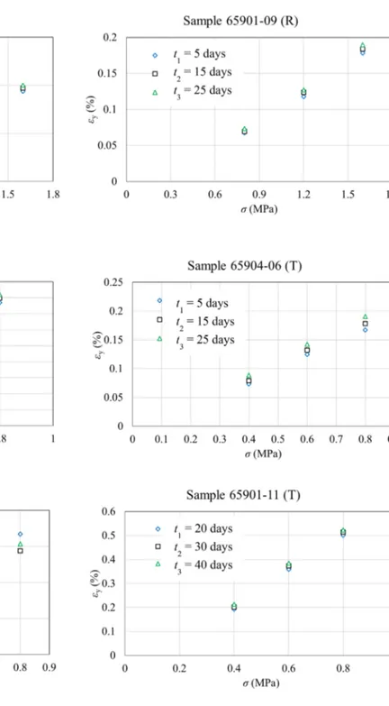
of the load, whereas the more viscoelastic biopolymer matrix (lignin and hemicellulose) carries a proportion-ally larger share of the load in transverse loading, i.e. in the R and T directions (de Borst and Bader 2014). The stiff reinforcing cellulose predominantly oriented in the L direction shows an elastic behaviour, whereas the surrounding lignin–hemicellulose matrix shows a viscoelastic behaviour (Navi and Stanzl-Tschegg 2009). In the following, only the measurable creep in the trans-verse directions (R and T) is presented. The linearity of the curves for all of the samples in R and T-directions is shown in Fig. 8. Please note that the plots are intention-ally plotted as strain (dependent value) as a function of stress (independent value), since the stress is constant and the measured property is the resulting strain, with the slope being the creep compliance. Also note that for some of the samples, the data for time 30 and 40 days were missing. That is why two sets of time points are pre-sented in Fig. 7. However, a sensitivity analysis by choos-ing different time points showed no effect on the output parameter, i.e. stress threshold evaluation. As a result, a combination of time points was chosen to demonstrate the independence of the stress threshold from the selection of time points, as was expected.
It can be seen from Figure 8 that all the samples, with the exception of sample 65900-01, show a linear rela-tionship between stress and strain. By linear fitting of the data, the threshold stress for each orthogonal direc-tion was calculated. The threshold stress in T direcdirec-tion is between 0.05 and 0.2 MPa and in R direction between 0.3 and 0.5 MPa. As expected, R direction has a higher threshold stress due to relatively higher stiffness in com-parison to T direction, which can be attributed to the presence of stiffening rays in the R direction (de Borst et al. 2012). Although subject to a relatively large scatter in these ranges, average values of the threshold can be calculated, which were found to be 0.125 MPa in the T direction and 0.4 MPa in the R direction. If creep should be minimised, one can compare stresses from finite ele-ment simulations with these values for different relieving support systems.
4.3 Viscoelastic parameters
A summary of the viscoelastic parameters, i.e., relative modulus α and relaxation time τ for all of the samples can be found in Table 3. If R and T values are pooled together, the average and standard deviations of these parameters are given in Table 4.
First, some of the values of α and τ in Table 3 are outliers and should be interpreted with care. These are indicated by asterisk symbol. The main reason is that a negligible creep behaviour was observed in those samples (for example, in the case of samples 65901-09, 65904-06 and 65900-01).
Examining the values of α and τ with increasing stress level for each sample, a trend can be perceived. With increas-ing stress level, the relative modulus α becomes higher and the relaxation time τ becomes shorter. In Table 3, this trend is quite evident for sample 65901-11, 65904-06 (excluding the first load step), for sample 65900-01 (excluding the first load step and only in terms of τ) and for 65903-07 (exclud-ing the last load step).
When the creep results from the various relevant samples are pooled together for each direction and stress level, the same trends can be observed in Table 4, with the exception of the highest stress level in R-direction, where α decreases. However, the scatter is considerable, and the trends cannot be ascertained to any high level of statistical confidence. Overall values for the entire stress range are also presented in Table 4. Although the variation of the average values of the viscoelastic parameters with respect to the stress level may lead to believe that the material cannot be considered to be linearly viscoelastic, the similitude of the isochronous stress–strain relations and the creep compliance (an engi-neering property) shown in Fig. 8 implies that the assump-tion of linearity is justified in regard to the generally high variability in material properties. Therefore, the average values of α and τ are calculated and given for two directions of the wood (R and T) in Table 4, which are candidates for material parameters in a finite element model to predict structural creep deformation.
Finally, the results in Table 4 can be compared with some experimental data for other kinds of wood in the literature. Viscoelastic characterization in R and T directions is not widely reported, in particular for archaeological wood. In a study on viscoelastic characterization of wood, Ozyhar et al. (2013) investigated creep on samples made from European
Table 2 Stress–strain at each time point and corresponding compliance moduli for each stress level
Δσ (MPa) t1 = 20 days t2 = 30 days t3 = 40 days
εy (%) J (t) (MPa‒1) ε
y (%) J (t) (MPa‒1) εy (%) J (t) (MPa‒1)
0.4 0.193 0.481 0.202 0.504 0.213 0.533
0.6 0.359 0.599 0.373 0.621 0.384 0.640
beech wood (Fagus sylvatica) in the L, R and T directions. Their relative modulus α of 0.62 and 0.54 for R and T direc-tions, respectively corroborates with the present one. Fur-thermore, relaxation tests were performed by Hu and Guan (2019) for unaged beech wood (Fagus orientalis) in L, R and T directions. From their data, an average relative modulus
α of 0.33 and 0.51 for R and T directions, respectively, was
obtained. This is only in rough agreement with the present value of α = 0.62 in R-direction but in good agreement with
α = 0.58 in T-direction. The relaxation times τ were,
how-ever, not comparable for these studies. Polymer materials are known to show multiple relaxation times, which can be attributed to different deformation mechanisms (Ward and Sweeney 2004). The prominence of relaxation time for poly-mer material depends on the timeframe of the creep test. The chosen test times differed over several orders of magnitude, which means that comparison of relaxation times were not meaningful.
5 Conclusion
There is a general lack of available creep data for wood materials which could be used for predictions of long-term deformations of structures, although neglecting the time-dependent deformations is not justified (Ozyhar et al. 2013; Huč and Svensson 2018). This is particularly the case for archaeological wood materials, where there is little creep data available, despite the creep deformation in large wooden structures in cultural heritage. The results from compressive creep tests of oak samples from the Vasa ship essentially showed linearity in the viscoelastic material model (standard
linear solid) according to the Boltzmann superposition prin-ciple for small cubic samples loaded in T and R directions. In addition, the viscoelastic properties of the wood as well as a stress threshold, in which negligible creep is expected, were obtained. The creep behaviour of the samples loaded in longitudinal L direction was found to be negligible com-pared to that in the transverse R and T directions.
The obtained rheological parameters may serve as first input parameters in a user-defined material model in a finite-element analysis for creep deformation predictions of the entire ship. They would however need to be complemented by the coupling between the main material axes, i.e. Poisson numbers, and shear moduli.
Acknowledgements Open access funding provided by Uppsala Uni-versity. Financial support from the Swedish National Maritime and Transport Museums to R. A. and G. A. is gratefully acknowledged. Compliance with ethical standards
Conflict of interest The authors declare that there is no conflict of in-terest.
Open Access This article is licensed under a Creative Commons Attri-bution 4.0 International License, which permits use, sharing, adapta-tion, distribution and reproduction in any medium or format, as long as you give appropriate credit to the original author(s) and the source, provide a link to the Creative Commons licence, and indicate if changes were made. The images or other third party material in this article are included in the article’s Creative Commons licence, unless indicated otherwise in a credit line to the material. If material is not included in the article’s Creative Commons licence and your intended use is not permitted by statutory regulation or exceeds the permitted use, you will need to obtain permission directly from the copyright holder. To view a copy of this licence, visit http://creat iveco mmons .org/licen ses/by/4.0/.
References
Bjurhager I, Halonen H, Lindfors E-L et al (2012) State of degrada-tion in archeological oak from the 17th century Vasa ship: sub-stantial strength loss correlates with reduction in (holo)cellulose molecular weight. Biomacromology 13:2521–2527. https ://doi. org/10.1021/bm300 7456
Cederlund CO, Hocker FM (2007) Vasa I: the archaeology of a Swed-ish Warship of 1628. Int J Naut Archaeol 36:426–429. https ://doi. org/10.1111/j.1095-9270.2007.163_1.x
de Borst K, Bader TK (2014) Structure–function relationships in hard-wood—insight from micromechanical modelling. J Theor Biol 345:78–91. https ://doi.org/10.1016/j.jtbi.2013.12.013
de Borst K, Bader TK, Wikete Ch (2012) Microstructure–stiffness rela-tionships of ten European and tropical hardwood species. J Struct Biol 177:532–542. https ://doi.org/10.1016/j.jsb.2011.10.010
Hocker E (2010) Maintaining a stable environment: Vasa’s new cli-mate-control system. J Preserv Technol 41:3–9
Hocker E, Almkvist G, Sahlstedt M (2012) The Vasa experience with polyethylene glycol: a conservator’s perspective. J Cult Herit 13:S175–S182. https ://doi.org/10.1016/j.culhe r.2012.01.017
Hoffman P (2013) Conservation of archaeological ships and boats. Archetype Publications Ltd, London
Table 3 Viscoelastic parameters for all samples in R and T directions
a The values are outliers
Sample (direction) Stress level (Δσi) (MPa)
Relative
modulus α Relaxation time τ (days)
65901-09 (R) 0.8 0.11a 2.10a 1.2 0.51 29.00 1.6 0.39 20.00 65903-07 (R) 0.8 0.65 26.30 1.2 0.86 11.70 1.6 0.72 19.00 65905-01 (T) 0.4 0.49 33.70 0.6 0.73 12.00 0.8 0.70 17.16 65904-06 (T) 0.4 0.83a 0.50a 0.6 0.73 11.00 0.8 0.83 6.64 65900-01 (T) 0.4 0.10a 0.26a 0.6 0.61 12.40 0.8 0.57 10.10 65901-11 (T) 0.4 0.38 15.80 0.6 0.51 12.00 0.8 0.59 8.80
Table 4 Viscoelastic parameters in terms of average and standard deviation of relative modulus α and relaxation time τ
Loading
direc-tion Stress level (Δσi) (MPa)
Relative
modu-lus α Relaxation time τ (days)
R 0.8 0.65 26.30 1.2 0.68 ± 0.25 20.35 ± 12.23 1.6 0.55 ± 0.23 19.5 ± 0.71 Average 0.62 ± 0.07 22.05 ± 3.70 T 0.4 0.43 ± 0.07 24.75 ± 12.65 0.6 0.64 ± 0.10 11.85 ± 0.59 0.8 0.67 ± 0.10 10.78 ± 7.76 Average 0.58 ± 0.13 15.79 ± 7.77
Hoffmann P (2009) On the stabilization of waterlogged oakwood with polyethylene glycol (PEG) III. Testing the oligomers. Holzforsch Int J Biol Chem Phys Technol Wood 42:289–294. https ://doi. org/10.1515/hfsg.1988.42.5.289
Hu WG, Guan HY (2019) Study on compressive stress relaxation bahavior of beech based on the finite element method. Maderas Cienc Tecnol 21:15–24. https ://doi.org/10.4067/S0718 -221X2 01900 50001 02
Huč S, Svensson S (2018) Coupled two-dimensional modeling of vis-coelastic creep of wood. Wood Sci Technol 52:29–43. https ://doi. org/10.1007/s0022 6-017-0944-3
Jones A, Rule M, Jones E (1986) Conservation of the timbers of the tudor ship Mary rose. Biodeterioration 6. CAB International, Washington, DC
Navi P, Stanzl-Tschegg S (2009) Micromechanics of creep and relaxa-tion of wood. A review COST Acrelaxa-tion E35 2004–2008: wood machining—micromechanics and fracture. Holzforschung. https ://doi.org/10.1515/HF.2009.013
Ozyhar T, Hering S, Niemz P (2013) Viscoelastic characteriza-tion of wood: time dependence of the orthotropic compliance in tension and compression. J Rheol 57:699–717. https ://doi. org/10.1122/1.47901 70
Shipsha A, Berglund LA (2007) Shear coupling effects on stress and strain distributions in wood subjected to transverse compression.
Compos Sci Technol 67:1362–1369. https ://doi.org/10.1016/j. comps citec h.2006.09.013
van Dijk NP, Gamstedt EK, Bjurhager I (2016) Monitoring archaeo-logical wooden structures: non-contact measurement systems and interpretation as average strain fields. J Cult Herit 17:102–113.
https ://doi.org/10.1016/j.culhe r.2015.03.011
Vorobyev A, van Dijk NP, Kristofer Gamstedt E (2019) Orthotropic creep in polyethylene glycol impregnated archaeological oak from the Vasa ship. Mech Time-Depend Mater 23:35–52. https ://doi. org/10.1007/s1104 3-018-9382-3
Ward IM, Sweeney J (2004) An introduction to the mechanical proper-ties of solid polymers, 2nd edn. Wiley, Chichester
Zhang J-S (2010) Creep of particulates reinforced composite mate-rial. In: High temperature deformation and fracture of materials. Woodhead, Illinois, pp 102–110
Publisher’s Note Springer Nature remains neutral with regard to jurisdictional claims in published maps and institutional affiliations’.